J. of the Braz. Soc. of Mech. Sci. & Eng. Copyright 2009 by ABCM July-September 2009, Vol. XXXI, No. 3 / 173
! " # "$# % &
! " # "$# % &
A phase-field model is proposed for the simulation of microstructure and solute concentration during the solidification process of Fe-C-P ternary alloys. A relation between material properties and model parameters is presented. Two-dimensional computation results exhibit dendrites in Fe-C-P alloys for different phosphorus concentrations. Alterations in the phosphorus concentration appear to affect the advance speed of the solid-liquid interface. Such an alteration is due to the small diffusivity of phosphorus during the solidification process.
Keywords: phase field, solidification, ternary alloys, dendrite, simulation
Introduction
1
For a number of years now, appreciable attention has been paid, in open literature, to the simulation of dendrite growth and related phenomena. Several different numerical approaches were proposed to that end. Some works have focused on pure materials, whereas others took heed of binary alloys of metallurgical interest. One example is the work by Warren and Boettinger (1995), which applies the Phase-Field Method to such problems. Another approach employing adaptive finite elements can be found in Narski and Picasso (2007). At the same time, results have been published pertaining to phase-field modeling and simulation of anisotropy effects (Suwa et al., 2007) and solidification processes (Mullis, 2006). On the other hand, some work has been performed on segregation in ternary alloys (Wynblatt and Landa, 1999). It is in this general framework that the present work is developed, with a focus on ternary alloys and Phase-Field Method implemented via finite volumes.
Solidification is the main phenomenon taking place during casting. This, in turn, has long been known as a relatively inexpensive means for producing metal goods. Nowadays, a sizable portion of the concepts and methods developed over the years in support of the research into solidification phenomena can be successfully and economically translated to industrial scale. Noticeable improvement can thereby be achieved, insofar as the quality of the pieces manufactured by solidification is concerned. For this reason, solidification studies are not just mandatory; they truly are a powerful industrial tool. For conventional technologies, through understanding and control of the solidification process opens wide perspectives in terms of its economic potential, since it provides the shortest distance from metal input to final product. As a consequence, solidification is one of the most important specialties in Metallurgy and Materials Science.
In-the-mold solidification of a metal, opposite to what might at first be surmised, is not a “passive” process in any way. On the contrary, the metal undergoes a liquid-to-solid transformation of very dynamic nature. In its course, events take place — like nucleation and growth of dendritic structures — which, in the absence of a tight control, may compromise the final output or even halt the manufacturing process altogether. Such events can originate several types of material heterogeneities which drastically affect the metallurgical quality of the final product. Therefore, solidification and the main structures arising from it — the dendrites — are extremely important from a practical standpoint, in that they exert a strong influence on the properties of the products.
Paper accepted September, 2008. Technical Editor: Amir A. M. Oliveira Jr.
Often, in situations that reflect more closely the conditions in applications, it is not feasible to obtain solutions using classical mathematical models of solidification. Usually, analytical solutions are possible only in very limited and idealized situations such as one-dimensional solidification, constant diffusion coefficients, liquid at saturation temperatures, same density and heat capacities of solid and liquid phases. On the other hand, even more detailed numerical models using classical equations can hardly resolve complicated two- and three-dimensional dendrite structures. Also, methods based on classical transport equations are found to be limited, when dealing with meta-stable states. Pure substances provide one such example, when the solidification front advances through a super-cooled liquid phase. Another case is that of alloy solidification, for instabilities of the advancing front can occur owing to constitutional super-cooling. In these instances, the solid-liquid interface may develop a complex geometry, locally dependent on curvature, solidification speed, and possible anisotropy. For this reason, over the past twenty years, considerable effort has been applied to the ad hoc development of specialized physical and numerical methods.
In particular, the Phase-Field Method has garnered wide acceptance, given its ability to simulate the solidification process in the presence of a complicated solid-liquid interface. The seminal work on the method is due to G. Caginalp and co-workers (Caginalp and Fife, 1986), dating back to the early 1980’s. A collection of models has stemmed from that paper, ever since. At first, the focus was on pure materials (Kobayashi, 1993; Kim et al., 1999; Furtado et al., 2006) and then, on binary alloys (Lee and Suzuki, 1999; Ode and Suzuki, 2002). Usually, in phase-field works, solutions to the equations are obtained by divided differences. For alloys, dendrite growth is considered at constant temperature or constant cooling rate. In our work, all equations were solved numerically with recourse to the Finite-Volume Method (Patankar, 1980). The reason for such a choice lies in the fact that this is a conservative method. The transient term of the phase field equation is discretized using an explicit scheme since it does not need to be solved in both the solid and liquid regions. It suffices to solve the equation around the interface. For the transient term in the energy conservation equation, an implicit scheme is used, owing to its unconditional numerical stability regardless of the size of the time step used. In all of our simulations, a single, stable, solid nucleus is considered to have been previously added to the liquid domain. Moreover, for applying the Phase-Field Method to the solidification of Fe-C-P ternary alloys, we prescribe as initial conditions the temperature and solute concentration, taking into account surface tension and crystal anisotropy effects.
that it tends to render steels fragile, especially high-carbon steels or when their content goes beyond certain acceptable limits (Chalmers, 1964). For this reason, the maximum admissible phosphorus content is specified.
Nomenclature
A = noise amplitude, dimensionless Cp = specific heat, J/ m3K
D = thermal diffusivity, m2/s Fs = solid fraction, dimensionless
g =models interface surface tension, dimensionless h = smoothing function, dimensionless
j =controls the number of preferential growth directions J = number of preferential growth directions, dimensionless t = time, s
ke = equilibrium partition coefficient, dimensionless
R = universal gas constant, J/mol.K t = time, s
T = temperature, K Vm = molar volume, m3/mol
W = excess free energy, J/m3 Greek Symbols
δε =gauges the anisotropy, dimensionless ∆H = latent-heat variation, J/m3
ε = interface thickness, (J/m)1/2 φ = order parameter, dimensionless λ = interface thickness, m
θ = growth angle, deg. σ = interface energy, J/m2 Subscripts
C relative to concentration of carbon
CL relative to concentration of carbon in the liquid region CS relative to concentration of carbon in the solid region m relative to molar concentration
p relative to pressure
P relative to concentration of phosphorus
PL relative to concentration of phosphorus in the liquid region PS relative to concentration of phosphorus in the solid region
Superscripts e equilibrium
Mathematical Model
We solve simultaneously the equations of energy, phases, and carbon and phosphorus concentrations. Use of the Phase-Field Method presupposes occurrence of growth of one or more solid nucleus in the bulk of the liquid phase. Here, in particular, one of such nucleus is assumed to grow. As a consequence, three different regions that exist must be considered, namely the solid and liquid regions as well as their interface.
The energy equation to be integrated is (Furtado et al., 2006)
( )
t h C H T D t T p ∂ ∂ ′ ∆ + ∇ = ∂∂ 2 φ φ
(1)
The term on the left-hand side represents the time variation of the specific thermal energy divided by the constant pressure specific heat. The first term on the right-hand side is the divergence of the heat transfer by heat diffusion (conduction) divided by the product of specific mass and constant pressure heat capacity, where D is the thermal diffusivity and T represents the temperature. The second
term on this side is a source, where Cp is the specific heat at constant
pressure, ∆H measures the latent-heat variation around the interface and h’(φ ) is the derivative of the so-called “smoothing” function, to be defined later. The derivative ∂φ⁄ ∂t is the time-and-space rate of variation of the phase-field variable, φ.
As for the phase equation, Ode et al. (2000) propose
(
)(
)
noise c c c c c c c c Ln V RT h g w t M PS CS e PL e CL PL CL e PS e CS m + + − + − + − + − ′ + ′ − ∇ = ∂ ∂]
[
]
[
]
[
]
[
) ( ) ()
(
)
(
1 1 1 1 ) ( ) (1 2 2
φ φ φ ε φ (2)
The evolution of the solid nucleus with time (∂φ⁄ ∂t) is assumed to be proportional to the variation of the free-energy functional with respect to the order parameter, φ. The terms of the phase equation are derived from this free-energy functional, which must decrease during any solidification process, as indicated in the article by Furtado et al. (2006). In Eq. (2), M quantifies the phase-field mobility. The product ε2∇2φ is a diffusivity term. The next component of the equation, wg’(φ), factors in the excess free energy arising from surface tension around the interface. The last product on the right-hand side translates the driving force behind the solidification process. Here, R is the gas constant and Vm, the molar
volume. The arguments to the natural logarithms, ceCS and cePS, are, respectively, the equilibrium concentrations of carbon and phosphorus in the solid region. Likewise, ceCL and c
e
PL represent their corresponding equilibrium concentrations in the liquid phase. Their respective ordinary concentrations in the liquid and solid regions are denoted, by the pairs cCL and cPL, and cCS and cPS. The noise term in the right-hand side of the phase-field equation will be explained later.
As proposed by Ode et al. (2000), solute concentrations in both regions are calculated with the solute transport equations, numbered (3) and (4), below.
( )
[
]
[
]
[
]
+ − ∇ − + − + − + − − ∇ = ∂ ∂ •)
(
)
(
)
(
L P L C L C S P S P S C S C L P L P L C L C C C c c c Ln c c c c h c c c c h D t c 1 1 1 ) ( 1 1 ) ( 1 φ φ φ (3)( )
[
]
[
]
[
]
+ − ∇ − + − + − + − − ∇ = ∂ ∂ •)
(
)
(
)
(
L P L C L P S C S P S C S p L C L P L C L p P P c c c Ln c c c c h c c c c h D t c 1 1 1 ) ( 1 1 ) ( 1 φ φ φ (4)In these equations, DC and DP are the carbon and phosphorus
diffusivities in the solid and liquid regions. The model used here takes into account solute diffusivity in the liquid and interface regions.
J. of the Braz. Soc. of Mech. Sci. & Eng. Copyright 2009 by ABCM July-September 2009, Vol. XXXI, No. 3 / 175
(
2)
3
6 15 10 )
(φ =φ − φ+ φ
h (5)
(
)
22 1 )
(φ =φ −φ
g (6)
Equations (5) and (6) are widely employed in phase-field works. Notice h’(φ) and g’(φ) are zero for both φ = 0 (liquid region) and φ = +1 (solid region). This ensures that only at the interface will the second and third terms in Eq. (2) be nonzero. Moreover, a commonly resorted way of including anisotropy in the model is to regard ε in Eq. (2) as dependent on a so-called “growth angle,” θ. The growth angle reflects the orientation of the normal to the interface with respect to the x axis, i.e., the longitudinal interface advance direction (Furtado, 2005):
(
)
[
]
{
0}
0 1 cos
)
(
θ
ε
δ
θ
θ
ε
= + ε j − (7)where δε gauges the anisotropy. The value j controls the number of preferential growth directions. For example, with j = 0 we shall be looking at a perfectly isotropic case, while j = 4 is indicative of a dendrite with four preferential growth directions. Orientation of the maximum-anisotropy interface is identified by the θo constant of Eq.
(7). Furthermore, εo in that equation, and w in Eq. (2) are model
parameters associated with interface energy (σ) and thickness (λ), respectively, according to the following expressions (Furtado, 2005):
∫
= = 9 , 0 1 , 0 0 0 0 2 2 . 2 d d d 2 w x ε φ φλ (8)
2 3 d 0 2 0 2 0 w x x ε φ ε σ λ λ = ∂ ∂ =
∫
+ − (9)Also from Furtado (2005), the phase-equation mobility, M, is computed as
(
)
(
)
+ = e S e L i e S e L i c c D c c D wM 2 2 2 2
1 1 1 1 3 0 , 1 , 1 2
1 ξ ξ
σ ε
(10)
where each of the ξ j is obtained from
(
)
− × − + − − − × − =∫
)
(
)
(
)
(
]
[
]
[
0 0 0 10 0 0
0 0 2 1 d 1 ) ( 1 ) ( 1 ) ( 1 ) ( φ φ φ φ φ φ φ ξ e jS e jS e jL e jL e jS e jL m j c c h c c h h h c c V RT (11)
In Eqs. (10) and (11), L and S stand for liquid and solid, respectively.
To simulate growth of an asymmetrical dendrite, it is necessary to introduce a noise term in the right-hand side of the phase-field equation. A usual expression for this noise, as indicated by Furtado (2005), is
(
)
22 1
16 φ −φ
= ar
noise (12)
where r is a random number between −1 and +1. The a parameter is the noise amplitude. Maximum noise corresponds to φ = 0.5, at the center of the interface, whereas at φ = 0 (liquid region) and φ = +1 (solid region) there occurs no noise. That is to say, noise is generated at the interface.
Results and Discussion
First off, we introduce phase-field results for the carbon and phosphorus concentrations in the solid region. These estimates shall later be compared with Scheil’s equation, here reproduced for convenience, as shown by Chalmers (1964):
(
)
10. .1
− −
= ke
s e
s c k F
c (13)
where cs and co are solid concentration and initial concentration in
the liquid, respectively, and FS is the solid fraction. In the present work, we assume the equilibrium partition coefficients (ke) in the ternary alloy system are the same as those of binary alloys.
Table 1 presents the physical properties of the alloy used in the computations that follow. Table 2 presents the parameters used in the Phase-Field Method.
Table 1. Physical properties of alloy (Ode et al., 2000).
Property C P Fe
Partition coefficient 0.204 0.102
Slope of liquids line, me (K/mol) 1802 1836
Diffusivity of solute in the liquid phase, DL (m2/s) 2.0 × 10⁻⁸ 1.7 × 10⁻⁹
Diffusivity of solute in the solid phase, DS (m2/s) 6.0 × 10⁻⁹ 5.5 × 10⁻¹¹
Interface energy, σ (J/m2) 0.204
Melting temperature, Tm (K) 1810
Molar volume, Vm (m3/mol) 7.7 × 10⁻⁶
Table 2. Computational parameters.
Anisotropy, δε 0.05
Interface thickness, εo (J/m)1/2 1.462 × 10− 4
Surface tension, w (J/m3)
1.346 × 10 6
Interface mobility, M (m3/sJ) 0.393
Grid spacing, ∆x = ∆y (m) 3 × 10− 8
Time-step length, ∆t (s) 1 × 10− 9
The boundary condition adopted for the Phase-Field Method (φ) in this work is a zero-flux condition. Adiabatic boundary conditions were used for integrating the energy equation.
Estimate of Solute Concentration in the Solid
In preparing this article, the authors placed appreciable attention on the choice of a suitable computational grid. Even if not too sharp, an interface may still be fine enough to capture correctly the phenomena that occur there. Thus, a major effort has been made to obtain a sufficiently large number of nodal points around the interface so that phase-field gradients can be captured, for it is these gradients that define the temperature and concentration fields. In order to do that, a square mesh (dimensions: ∆x = ∆y = 3 × 10⁻⁸ m) has been used. With such dimensions, the phase-field solution converges with six nodal points inside the interface, which is sufficient for capturing phase-field gradients. More refined grids would require a larger computation domain, entailing greater computational effort. On the other hand, less refined grids would result in a diverging phase-field solution.
Results for solute concentration in the solid region during the solidification are presented in this section. Figure 1 shows the evolution of the solid fraction (FS) with time for an initial temperature of 1770 K. This solid fraction is given by the ration of the solid control volume to the total control volume of the domain, as shown in the following expression:
(
S L)
S V V
F =100 (14)
Figure 1. Solid fraction (FS) versus time.
A thin solid layer was added at the left boundary of the rectangular domain. In the next figure, the solid line represents fit, which is dependent upon a function of the square root of the time, whereas the points represent the values computed with the phase-field model.
In Fig. 1, the solid fraction (FS) is seen to increase faster at the onset of solidification. This rate then gradually diminishes towards completion of the solidification process. This slowing down is due to a reduction of interface mobility as the temperature increases. Given that we are considering adiabatic boundary conditions, owing to liberation of latent heat during the change of phase, an increase of the temperature occurs as a consequence of the reduction of the interface mobility. Traditionally, one assumes that the solid fraction (FS) is proportional to the square root of time, as any diffusion- controlled growth process (Chalmers, 1964). In the present calculation, interface motion is determined from the thermodynamic driving force, represented by the third term in Eq. (2). Results in
Fig. 1 display good agreement between the calculated fraction and the square root of the time at the beginning of the solidification. But, as expected, the behavior is clearly nonlinear, with both curves tending upwards as the solid fraction (FS) increases.
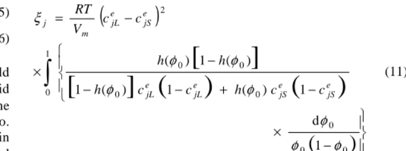
Figure 2 exhibits a comparison of the carbon concentration as evaluated by the model for the solid region and Scheil’s equation, cited in Chalmers (1964). We can see that phase-field-based results lie above those obtained with Scheil’s equation. For the latter, a complete mixing is assumed of carbon in the liquid and without diffusion in the solid. For the Phase-Field Method, carbon diffusivity in both the liquid and the solid are admitted. When carbon diffusivity in the solid is considered, one observes an enrichment of the solid region in the course of the solidification. At the end of the process, the phase-field estimate of the carbon concentration falls below Scheil’s curve. If the same diffusivity for the liquid phase was to be adopted by both the phase-field model and Scheil’s equation, the two curves would be in good agreement. However, Scheil’s equation takes into account a complete mixing of solute in the liquid. Thus, the liquid being homogeneous, the amount of material solidified, and hence of solute retained in the solid, will be smaller. The Phase-Field Method, on the other hand, assumes, for the solute in the liquid, a diffusivity on the order of 10−9 m2/s. Therefore, just ahead of the moving interface, an accumulation of solute takes place, yielding a greater solute concentration in the liquid next to the interface as compared to the results from Scheil’s model. Also, the presence of the cs=ke.cl law in the phase-field formulation will give a greater solute concentration in the solid than predicted by Scheil’s equation. Since both laws for cs admit a mass balance, in the final steps of the solidification process, Scheil’s model will indicate a greater concentration of solute remaining to be solidified, as shown in Fig. 2.
Figure 2. Comparison of carbon concentration, as evaluated via the Phase-Field Method, with Scheil’s equation, mentioned in Chalmers (1964).
J. of the Braz. Soc. of Mech. Sci. & Eng. Copyright 2009 by ABCM July-September 2009, Vol. XXXI, No. 3 / 177
Figure 3. Comparison of phosphorus concentration, as evaluated via the Phase-Field Method, with Scheil’s equation (Chalmers, 1964).
The next section features results of a study on the carbon and phosphorus diffuse layer in the liquid region.
Simulation of the Diffuse Layer of Solute in the Liquid Phase
In this simulation, the initial domain temperature is 1770 K. A “seed” (solid nucleus) is previously added at the bottom of the domain (Y = 0, X = 2.25 × 10⁻⁶
m). Preferential growth angle of the dendrite tip is 90º to the x axis. Anisotropy mode is J = 4. Initial molar concentration of carbon and phosphorus are, respectively, 0.5% and 0.001%. A dendrite tip is shown in Fig. 4.
Figure 4. Start of dendrite growth, t = 4××××10−−−− 7 s.
The dark region represents the solid and white stands for remaining liquid. The interface is the gray area between the solid and liquid regions. Dendrite tip dimensions (in this case): base width, 0.5 × 10⁻⁶ m; height, approximately 0.35 × 10⁻⁶ m. The curves of carbon and phosphorus content extracted from the dendrite tip are shown in the next figure (Fig. 5).
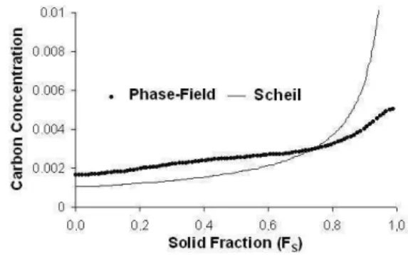
Figure 5. Carbon and phosphorus concentrations by region: solid (φφφφ = +1), liquid (φφφφ = 0), and interface (0 <φφφφ < +1).
Plots in Fig. 5 correspond to 4 × 10⁻⁷ s of solidification time. The left-hand vertical axis gives the carbon concentration; the right-hand one, that of phosphorus. When φ = +1, we are in the solid region, whereas φ = 0 is the liquid. The interface lies between φ = +1 and 0. Therefore, one can see that the solid region is poor in both carbon and phosphorus. This is because, during solidification, the solutes are rejected into the liquid phase, which then becomes rich in solute just ahead of the interface. As we move farther to the right, hence away from the interface, concentration decreases exponentially for both solutes, towards their initial values in the liquid. Such tendency seems to be in agreement with the consideration that the Gibbs free energy is more negative in the solid phase. Still with respect to Fig. 5, one can observe the carbon diffuse layer to be larger than that of phosphorus, due to the greater diffusivity of carbon as compared to that of phosphorus. As for the seeming coincidence in the peak percentage concentrations, it merely stems from the fact that the carbon axis, to the left, features a scale two orders of magnitude greater than that for the phosphorus, to the right.
Figure 6 presents the carbon profile in the course of the solidification process, at t1 = 1.0 × 10−
6
s, t2 = 2.25 × 10− 6
s, and t3 =
5.0 × 10⁻⁶
s from the inception of solidification. In this picture, one can see the concentration peak advance along the abscissas axis for t1, t2, and t3 and, as a result, an increase in the carbon concentration
peak. On all three curves, right prior to the peak, enrichment in solute can be observed in the solidified region. As mentioned before, this follows because, in the Phase-Field Method, solute diffusivity in the solid is admitted. After the peak, the carbon concentration decays exponentially to its value in the liquid phase, i.e., co = 0.5%. The diffuse layer undergoes no significant alteration
in thickness, whereas the carbon concentration peak increases with times t1, t2, and t3. It happens because solubility in the solid is less
Figure 6. Carbon concentration profile at times t 1, t 2, and t 3.
Microstructure Simulation of the Fe-C-P Alloy
Figure 7 displays results obtained with a microstructure simulation of a Fe-C-P dendrite with 0.5% C and 0.001% P. Boundary and initial conditions are the same as in Sec. 3.2, except that the initial temperature is now 1750 K.
Figure 7. Dendrite simulated for a super-cooled domain.
The dendrite exhibited in Fig. 7 was calculated from a seed previously added to the domain at Y = 0 and X = 0.75 × 10⁻⁵ m. Three different preferential growth directions can be discerned, the growth time being 2.75 × 10⁻⁵ s. Dendrite growth speed depends
upon the initial super-cooling (∆T = Tinitial – Tfusion), as discussed by
Furtado et al. (2006). In general, a sizable unbalance of Gibbs free energy occurs at the interface when there is intense supercooling. It is ultimately this unbalance that dictates the solidification speed. The dendrite shown above features some experimental characteristics described in the literature (Chalmers, 1964), which are secondary arms, outgrowths roughly perpendicular to the primary arms.
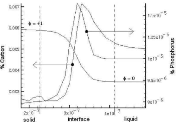
Figure 8 displays the carbon and phosphorus concentration distributions that correspond to the dendrite in Fig. 7. It can be seen that phosphorus concentration is much less than that of carbon. The carbon diffuse layer is more extensive than the phosphorus one. As before, this is explained by the carbon solute diffusivity being higher than the corresponding value for phosphorus. During solidification, there occurs, first in the liquid region, a variation of
the carbon concentration. Only thereafter does the phosphorus concentration vary. A carbon and phosphorus entrapment can be observed in the region next to the secondary arms. Therefore, these regions are the richest in both solutes. As a result, the solidification temperature is lower for those regions. With a greater solute (especially carbon) concentration and lower solidification temperatures, these will tend to be the last parts of the dendrite to solidify.
(a) carbon
(b) phosphorus
Figure 8. (a) Carbon and (b) phosphorus concentration fields.
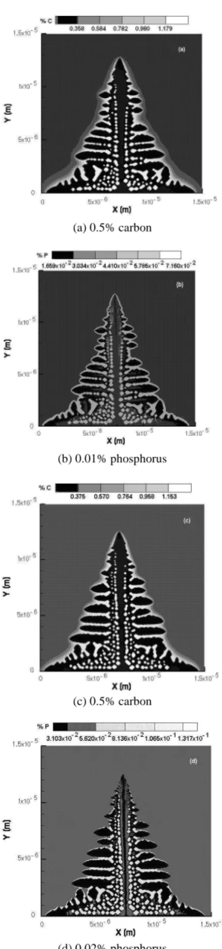
Next, the four images in Fig. 9 correspond to simulations carried out, separately, for the following two alloys: 0.5% C – 0.01% P; and 0.5% C – 0.02% P. The focus of these simulations was on the dendrite geometry as a function of the phosphorus content. However, as it can be seen by doubling the phosphorus content in the alloy, the geometry remained practically unaltered. The dendrite arm thickness suffered no significant change.
J. of the Braz. Soc. of Mech. Sci. & Eng. Copyright 2009 by ABCM July-September 2009, Vol. XXXI, No. 3 / 179 (a) 0.5% carbon
(b) 0.01% phosphorus
(c) 0.5% carbon
(d) 0.02% phosphorus
Figure 9. Carbon and phosphorus solute concentration fields. (a) and (b) 0.5% C – 0.01% P alloy; (c) and (d) 0.5% C – 0.02% P alloy.
Influence of Phosphorus Content on the Solidification Speed
For this simulation, boundary and initial conditions are the same as in the previous section, except that phosphorus content has been altered for evaluating the speed at each point for each set of initial and boundary conditions. Figure 10 shows the results. The speed can be seen to decrease monotonically as the phosphorus concentration increases. This occurs because phosphorus tends to reduce interface mobility, acting as a barrier against its motion. The apparent tendency toward a linear behavior in the speed plot is a mere consequence of the short time interval considered here.
Figure 10. Speed of dendrite tip versus phosphorus concentration.
Conclusions
Results for solid fraction (FS) against time at solidification onset are in agreement with the kinetic theory of solidification. That is, the solid fraction is roughly proportional to the square root of time. Curve separation is due to a loss of interface mobility as the domain temperature increases owing to liberation of latent heat.
Solute (both carbon and phosphorus) concentrations as calculated by the Phase-Field Method differ slightly from values obtained with Scheil’s equation. This occurs because our model takes into account solute diffusivity in the solid and liquid phases. As a result, the solid portion continues to be enriched with solute throughout the solidification process. Phase-field calculations for solute diffusivities yield a thicker diffuse layer for carbon, since this element has a greater diffusivity than phosphorus.
Two-dimensional simulations produced dendrites, which are similar to the ones found in experiments reported in the literature, complete with primary and secondary arms. During solidification, carbon and phosphorus are entrapped between the secondary arms. This effect lowers the solidification temperature in those regions, which, in turn, require a longer time to solidify.
melts slightly above 1000ºC. This, in turn, may cause steel rupture when hot-deformed.
On the basis of what has just been discussed, some prospects for future work include:
1) In spite of the ability of phase-field models to dendritic microstructure evolution during solidification, the method is plagued by low computational efficiency. For instance: with too refined grids, simulation of the evolution of a single dendrite would require a very large computation domain, with a million nodes. An option to circumvent this problem would be the implementation of adaptive grids, with a finer mesh around the interface.
2) This article features the evolution of a single dendrite, growing along some preferential directions. In future works, one could formulate simultaneous evolution of several dendrites growing in random directions. That way, it is possible to study the phenomenon of competitive growth of dendrites, which grew and developed along different directions. Then, there will be some dendrites more developed than others, as the latter shall have their growth inhibited.
Acknowledgments
The authors wish to thank Universidade Federal Fluminense (UFF) and, in particular, its School of Industrial and Metalurgical Engineering (EEIMVR), and Fundação de Amparo à Pesquisa do Estado do Rio de Janeiro (FAPERJ) for financial support and the necessary infrastructure for developing this research.
References
Caginalp, G., and Fife, P., 1986, “Phase-field methods for interface boundaries”, Physical Review B, Vol. 33, pp. 7792-7794.
Chalmers, B., 1964, “Principles of Solidification”, Wiley, New York, United States, p. 126.
Furtado, A.F., 2005, “Modelamento do Processo de Solidificação e Formação de Microestrutura pelo Método do Campo de Fase” (Phase-
Field Modelling of the Solidification and Microstructure Formation Process; in Portuguese), Ph.D. Thesis, Universidade Federal Fluminense, Volta Redonda, RJ, Brazil, p. 15.
Furtado, A.F., Castro, J.A., and Silva, A.J., 2006, “Simulation of the solidification of pure Nickel via the phase-field method,” Materials
Research, Vol. 9, pp. 349-356.
Kim, S.G., Kim, W.T., Lee, J.S., Ode, M., and Suzuki, T., 1999, “Large scale simulation of dendritic growth in pure undercooled melt by phase-field model,” ISIJ International, Vol. 39, pp. 335-340.
Kobayashi, R., 1993, “Modeling and numerical simulations of dendritic crystal growth,” Physical D, Vol. 63, pp. 410-423.
Lee, J.S., and Suzuki, T., 1999, “Numerical simulation of isothermal dendritic growth by phase-field model”, ISIJ International, Vol.39, pp. 246-252.
Mullis, A.M., 2006, “The effect of the ratio of solid to liquid conductivity on the side-branching characteristics of dendrites within a phase-field model of solidification”, Computational Materials Science, Vol. 38, pp. 426–431.
Narski, J., and Picasso, M., 2007, “Adaptive finite elements with high aspect ratio for dendritic growth of a binary alloy including fluid flow induced by shrinkage”, accepted in Computer Methods in Applied Mechanics and
Engineering; preprint available at http://iacs.epfl.ch/~picasso/NarskiPicasso.pdf.
Ode, M., Lee, J.S., Kim, S.G., Kim, W.T., Suzuki, T., 2000, “Phase-field model for solidification of ternary alloys”, ISIJ International, Vol. 40, pp. 870-876.
Ode, M., and Suzuki, T., 2002, “Numerical simulation of initial evolution of Fe-C alloys using a phase-field model”, ISIJ International, Vol. 42, pp. 368-374.
Patankar, S.V., 1980, “Numerical Heat Transfer and Fluid Flow”, McGraw-Hill-Hemisphere, New York, United States, p. 25.
Suwa, Y., Saito, Y., and Onodera, H., 2007, “Three-dimensional phase field simulation of the effect of anisotropy in grain-boundary mobility on growth kinetics and morphology of grain structure”, Computational
Materials Science, Vol. 40, pp. 40–50.
Warren, J.A., and Boettinger, W.J., 1995, “Prediction of dendritic growth and microsegregation patterns in a binary alloy using the phase-field model”, Acta Metall. Mater., vol.43, pp. 689-703.