Book-to-Market Ratio, return on
equity and Brazilian Stock Returns
Rebeca Cordeiro da Cunha Araújo
a,*aInstituto Federal de Educação, Ciênciae Tecnologia da Paraíba, João Pessoa, Brazil, and
Márcio André Veras Machado
bbUniversidade Federal da Paraíba, João Pessoa, Brazil
Abstract
Purpose–This study aims to analyze the influence of future expectations of the book-to-market ratio (B/M) and return on equity (ROE) in explaining the Brazilian capital market returns.
Design/methodology/approach–The study analyzed the explanatory power of risk-factor approach variables such as beta, size, B/M ratio, momentum and liquidity.
Findings– The results show that future expectations of the B/M ratio and ROE, when combined with proxies for risk factors, were able to explain part of the variations of Brazilian stock returns. With respect to risk factors approach variables, the authors verified the existence of size and B/M effects and a liquidity premium in the Brazilian capital market, during the period analyzed.
Research limitations/implications–This research was limited to the non-financial companies with shares traded at Brasil, Bolsa and Balcão, from January 1, 1995 to June 30, 2015. This way, the conclusions reached are limited to the sample used herein.
Practical implications–The evidences herein presented can also contribute to establishing investment strategies, considering that the B/M ratio may be calculated through accounting information announced by companies. Besides, using historical data enable investors, in a specific year, to calculate the predictor variables for the B/M ratio and ROE in the next year, which enhance the explanatory power of the current B/M, when combined in the form of an aggregate predictor variable for stock returns.
Originality/value– The main contribution of this study to the literature is to demonstrate how the expected future B/M ratio and ROE may improve the explanatory capacity of the stock return, when compared with the variables traditionally studied in the literature.
Keywords Anomalies, Risk factors, Return on equity, Fundamental valuation, Book-to-market ratio Paper typeResearch paper
1. Introduction
The efficient market hypothesis and the asset pricing models constitute one of the main pillars of the modernfinance theory. Despite much questioning about the assumptions of the asset pricing models, it is important to restate their theoretical and practical contribution to thefield offinance. Regarding corporatefinance, the asset pricing models allow determining
© Rebeca Cordeiro da Cunha Araújo and Márcio André Veras Machado. Published in RAUSP Management Journal. Published by Emerald Publishing Limited. This article is published under the Creative Commons Attribution (CC BY 4.0) licence. Anyone may reproduce, distribute, translate and create derivative works of this article (for both commercial and non-commercial purposes), subject to full attribution to the original publication and authors. The full terms of this licence may be seen at http://creativecommons.org/licences/by/4.0/legalcode
RAUSP
53,3
324
Received 11 October 2016 Accepted 31 October 2017
RAUSP Management Journal Vol. 53 No. 3, 2018
pp. 324-344
Emerald Publishing Limited 2531-0488
DOI10.1108/RAUSP-04-2018-001
The current issue and full text archive of this journal is available on Emerald Insight at:
the return rate used to assess alternatives of investment; concerning investment management, they are very much used to analyze risk and asset returns.
The capital asset pricing model (CAPM), developed bySharpe (1963,1964),Lintner (1965)
and Black (1972), is a single-factor model for which the beta can explain the differences in asset returns. Despite the simplifications imposed by its hypotheses, the CAPM is very useful for makingfinancial-related decisions because it quantifies and prices risk.
While developing tests to validate and apply the CAPM, the researchers found several regularities that the model did not explain. For this reason, they were named capital market anomalies. ToSchwert (2003), anomalies are empirical results that seem to be inconsistent with the asset pricing theories. They indicate either market inefficiency (profit opportunities) or inadequacies in the underlying asset-pricing model. Several approaches seek to explain market anomalies and analyze them from different perspectives.
The risk-factor approach considers that asset risk is multidimensional and thatfinancial indicators are factors that capture part of the systematic risk not covered by the CAPM. The exponents of this approach are the works ofFama and French (1992,1993), who developed a three-factor model using the following variables: market (CAPM beta),firm size (market value) and book-to-market ratio (B/M), that is, book value divided by market value.
Based on psychology and the limits-to-arbitrage concept, the behavioral approach considers that the causes of anomaly reside in investor irrationality. The momentum effect, proposed byJegadeesh and Titman (1993,2001), shows that the strategies to buy stocks that had good results in the past (Win) and sell stocks that had bad results in the same period (Los) generate significantly positive returns over the following months. Carhart (1997)
included momentum to the three-factor model ofFama and French (1993)and created that which is now known as the four-factor model.
Like the risk-factor approach, the fundamental valuation ofClubb and Naffi(2007)is based on the assumption that stocks are rationally priced. The difference between the former and the latter approach is that fundamental valuation is not based on the existence of a relation between a firm’s particular characteristic and its risk. Fundamental valuation seeks to demonstrate that many of the market anomalies are nothing but regularities in the relations across the said variables. Therefore, regardless of which process generates thefirm return, the empirically demonstrated relation between variables and returns will always be observed.
The fundamental perspective developed by Berk (1995, 1997) suggests that the traditional interpretation of the empirical relation between market value and average stock return may beflawed. Rather than the evidence of a“size effect”, the relation may occur because of an endogenous inverse relation between thefirms’market value and discount rate.Berk (1995)states that, if afirm’s market value is set, in equilibrium, as the discounted value of the expected future cashflows, it depends on a discount rate. Therefore, the bigger the cashflow discount rate (and, consequently, the bigger the expected return), the lower the market value will be. According to this view, the expected returns will always have a negative correlation with thefirms’market value,ceteris paribus.
Likewise, fundamental valuation considers the B/M ratio to be a more consistent variable thanfirm size to explain stock returns. According to this perspective, the relation between the B/M and the future returns is not given by the fact that B/M captures a risk factor but, rather, because it is a proxy for the expected cashflows, which correspond to an omitted term in the relation between market value and the expected returns.
Along the line of this approach, the study ofClubb and Naffi(2007)on companies of the UK from 1991 to 2000 suggests that the explanatory power of current B/M for future stock returns is enhanced by the inclusion of simple estimates of future B/M and return on equity (ROE) as additional explanatory variables. This way, this paper aimed to analyze the
Return on
equity and
Brazilian Stock
Returns
influence of the B/M ratio and expected future B/M ratio and ROE on explaining Brazilian stock market returns. As a comparison, this study analyzed the explanatory power of traditional pricing models, formed by the following variables: beta, size, B/M ratio, momentum and liquidity. Eventually, the three fundamental variables were checked for consistency through robustness tests, in which the variables of the two approaches were combined.
For this, the following hypotheses were tested:
H1. The B/M ratio explains part of the variations of Brazilian stock returns.
H2. The expected future B/M ratio explains part of the variations of Brazilian stock returns.
H3. The expected future ROE explains part of the variations of Brazilian stock returns.
These three fundamental variables are expected to explain part of the Brazilian stock returns; they are also expected to remain significant, even after including the risk-factor approach variables.
The results found in this paper may contribute to setting investment strategies, considering that the B/M ratio may be calculated through accounting information announced by the companies. In addition, using historical data enables investors, in a specific year, to calculate the variables to forecast the B/M ratio and the ROE for the following year, which enhance the explanatory power of the current B/M ratio, when combined in the form of aggregate predictor variable of the stock returns.
The main contribution of this study to the literature resides in focusing on Fundamental Valuation, which is an alternative perspective to analyze market anomalies that has few empirical evidences, especially in emerging countries. For the market, the results herein reported may contribute to setting investment strategies, considering that the fundamental variables under analysis may be calculated through accounting information announced by companies.
This paper includes five sections, including the introduction. Section 2 presents the theoretical framework and focuses on this study’s theoretical model, based on the Fundamental Analysis. Section 3 presents the methodological procedures used to reach the previously set objectives. Section 4 presents the results found on the empirical analysis. Finally, Section 5 conveys the conclusion.
2. Theoretical framework
The seminal work ofFama and French (1992) is a cornerstone of the study of efficient markets, asset pricing models and market anomalies. The authors demonstrated that size and B/M ratio have a greater explanatory power for stock returns than the CAPM beta estimates, and these variables have inspired numerous discussions on the role offinancial and accounting indices as predictors of stock returns.
The positive relation between the B/M ratio and the expected stock returns has been documented for decades, regardless of the adopted perspective. Under the risk-factor approach, the B/M factor is believed to explain part of the systematic risk variation not captured by the CAPM. On the other hand, the fundamental valuation assumes that the relation between the B/M ratio and future returns is not given by the fact that B/M captures a risk factor but, rather, because it is a proxy for the expected cashflows, corresponding to an omitted term in the relation between market value and expected returns (Berk, 1995;
1997).
Using data from the US market,Frankel and Lee (1998)found evidence of a variable for predicting B/M ratio. This variable, which incorporates market analysts’forecasts, had a
RAUSP
53,3
greater explanatory power than the book value, because it incorporated both past and present information. They also show that the relation between B/M and ROE is inverse. This occurs because the book value is a proxy for expected cashflows and, in a competitive equilibrium, afirm’s ROE should be close to its cost of equity capital (discount rate).Lee and Zhang (2014)ratified this evidence with data from the Chinese market.
Clubb and Naffi(2007)heightened this perspective, as they also focused on the role of ROE as a determinant of stock returns. They noted that the identity linking ROE, expected returns and B/M implies that expected stock returns for a period can be explained by a comparison of expected ROE and the expected change in the B/M ratio. This identity originated the fundamental analysis model to be analyzed in this study.
The logics underlying this argument is that inclusion of expected future ROE (in addition to current B/M) as an explanatory variable for stock returns, controls for cross-firm variation in current B/M caused by differences in expectations of short-term fundamental economic performance. Meanwhile, additional inclusion of expected future B/M as an explanatory variable for stock returns controls for the impact of expectations of longer term fundamental performance (Clubb and Naffi, 2007).
The B/M ratio relates both to thefirms’book value and market value. For this reason, it allows identifying its future perspectives both from the internal context and on the investors’view. In the fundamental perspective, the B/M is positively related to the stock returns, considering the book value as a proxy for thefirm’s future cashflows.
The fundamental analysis model ofClubb and Naffi(2007)is based on an identity that relates the current B/M ratio (t) and the expected future B/M ratio and ROE at timetþ1, assuming that the Clean Surplus Relation –CSR (accounting normative proposition for which afirm’s book value must be changed only as a function of dividends or profits) is valid for the net profits. The CSR may be described as follows:
BVt¼BVt 1þNPt Dt (1)
Where:
BVt = book value at timet;
NPt = net profits for the periodtþ1; and Dt = dividends paid at timetþ1.
The B/M ratio at timetþ1 for a specific company may be described as: BVtþ1þDtþ1
MVtþ1þDtþ1
¼ð1þROEtþ1ÞBVt
1þRt
ð ÞMV (2)
where:
MVt = market value at timet;
MVtþ1þDtþ1= (1þRt) MVtdenotes the market price at timetþ1; ROEtþ1 =NPBVttþ1denotes the ROE for the periodtþ1; and Rt = stock return for period t.
Applying a logarithmic transformation on this equation, we have:
ln 1ð þRtÞ ¼ln BVt MVt
ln BVtþ1þDtþ1 MVtþ1þDtþ1
þln 1ð þROEtþ1Þ (3) Taking the expectations at t ([.] represented by Et), wefind the expression for the logarithm of the expected stock returns for the period tþ1:
Return on
equity and
Brazilian Stock
Returns
Et½ln 1ð þRtÞ ¼ln BVt MVt
Et ln
BVtþ1þDtþ1 MVtþ1þDtþ1
þEt½ln 1ð þROEtþ1Þ (4) Which, in turn, implies the following equation for the logarithm of the realized returns in periodt:
ln 1ð þRtÞ ¼ln BVt MVt
Etln ln
BVtþ1þDtþ1 MVtþ1þDtþ1
þEt½ln 1ð þROEtþ1Þ þvt (5)
where:
vt= zero mean disturbance term.
Equation (5)provides the basis for the empirical analysis of this paper. The main objective was to verify whether this model, comprising the current B/M ratio, the expected B/M and ROE and a random disturbance term, explains stock return variations in Brazil. For this, this study used two regression models proposed byClubb and Naffi(2007):
RETT¼a0þa1BMt a2FBMtþ1þa3FROEtþ1þ«t (6)
where:
BMt = current B/M;
FBMtþ1 = expected future B/M; and FROEtþ1= expected future ROE.
RETT¼a0þa1FRMtþ1þ«t (7)
where:
FRMt= aggregate predictor variable FRM:BMt–FBMtþ1þFROEtþ1.
Equation (6)is a multivariate model andequation (7)is an aggregate univariate model, where, by definition, the explanatory variable FRM : BMt – FBMtþ1 þ FROEtþ1. According toClubb and Naffi(2007), the coefficients are expected to be within the following intervals: 0<a1<1, 0<a2< 1 and 0<a3<1 forequation (6)and 0<a1<1 for
equation (7). Although the model premises imply that the explanatory power of the stock returns for equations (6) and (7) should be identical, it is expected that differential measurement error in the proxy market forecast variables (FBMtþ1and FROEtþ1) will result in a difference of explanatory power across the two models (Clubb and Naffi, 2007).
Kothari (2001)and Lee (2001) convey a review of the academic literature on stock market anomalies and fundamental analysis before the year 2000, whileRichardsonet al.(2010)
conduct a similar research with studies after year 2000.Table Isums up the main empirical evidences, both national and international, on the relation between fundamental variables and stock return.
3. Methodological procedures 3.1 Population and sample
The sample comprised all thefirms listed at B3 (Brasil, Bolsa and Balcão), from January 1, 1995 to June 30, 2015. To guarantee the exactitude of the accounting data, somefilters were used. This way, this study excluded:financialfirms, because, according toFama and French (1992), their high leverage may distort the B/M ratio and it does not have the same meaning as for the high leverage of non-financialfirms;firms that did not have a market value on
RAUSP
53,3
December 31 and June 30 of each year;firms that did not have a positive book value on December 31 of each year;firms that did not have monthly quotations for 24 consecutive months. In the latter case, the 12 months prior to the beginning of each yeartwere used to calculate momentum, while the 12 months after that were used to calculate stock returns.
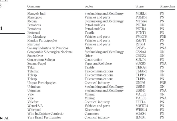
The analysis was based on individual assets. On average, 318 stocks were analyzed per year, which shows the reduced number of Brazilian companies whose stocks are traded at the Stock Exchange. As a comparison, the study ofClubb and Naffi(2007)analyzed, on average, stocks of 500 UKfirms each year, from 1991 to 2000. Considering that the predictor variables would be estimated through a linear dynamic panel, a balanced panel was put up for each analyzed company to have the same number of observations over time. Therefore, the sample included the stocks that had valid observations of the fundamental variables object of this study (B/M ratio and ROE), over the full period of analysis (19 years). Thus, the final sample comprised 89 stocks (28 per cent of the population, on average). The list of the firms comprising the sample can be found at theAppendix. It is important to underscore that analysis started in 1996, and that 1995 was used only to calculate the predictor variables. All the secondary data needed to conduct this study were taken from the Economatica database.
3.2 Model description
To compare the explanatory capacity of the fundamental variables presented in the previous section to the risk factors suggested in the literature, in addition to equations 6 and7
(Models 1 and 2, respectively), regression models were estimated and were formed on the following variables: beta (bt),firm size (market value) (SIZEt), B/M ratio (BMt), momentum
(MOMt) and liquidity (LIQt). Regression models estimated in this study sums up the main
regression models estimated in this study:
Table I. Main papers that analyze the relation between fundamental variables and stock return Variables
Empirical evidence Country B/M ROE Method
Fairfield (1994) USA X X Accounting valuation model
Ryan (1995) USA X B/M decomposition
Berk (1995) USA X Market value decomposition
Berk (1997) USA X Portfolio analysis/regression
Frankel and Lee (1998) USA X X Accounting valuation model
Pontiff and Schall (1998) USA X Regression analysis
Lev and Sougiannis (1999) USA X X Portfolio analysis/regression
Beaver and Ryan (2000) USA X X B/M decomposition
Billings and Morton (2001) USA X B/M decomposition
Vuolteenaho (2002) USA X X VAR model
Chen and Zhao (2006) USA X Portfolio analysis/regression
Clubb and Naffi(2007) UK X X Regression analysis
Fama and French (2008) USA X B/M decomposition
Almeida and Eid (2010) Brazil X B/M decomposition
Skogsvik and Skogsvik (2010) Sweden X Accounting valuation model
Dorantes (2013) Mexico X Portfolio analysis/regression
Lee and Zhang (2014) USA and China X Portfolio analysis/regression
Evrardet al.(2015) Brazil X X Forward selection regression/event study
Note:X = yes
Return on
equity and
Brazilian Stock
Returns
3.2.1 Regression models estimated in this study
(1) Fundamental valuation models:
Model 1:RETT¼a0þa1BMt a2FBMtþ1þa3FROEtþ1þ«t
Model 2:RETT¼a0þa1FRMtþ1þ«t
(2) Risk-factor approach models:
Model 3:RETT¼a0þa1btþ«t
Model 4:RETT¼a0þa1bt a2SIZEtþa3BMtþ«t
Model 5:RETT¼a0þa1bt a2SIZEtþa3BMtþa4MOMtþ«t
Model 6:RETT¼a0þa1bt a2SIZEtþa3BMtþa4MOMt a5LIQtþ«t
(3) Joint regression models:
Model 7:RETT¼a0þa1BMt a2FBMtþ1þa3FROEtþ1þa4btþ«t
Model 8:RETT¼a0þa1BMt a2FBMtþ1þa3FROEtþ1þa4bt a5SIZEt
þ«t
Model 9:RETT¼a0þa1BMt a2FBMtþ1þa3FROEtþ1þa4bt a5SIZEt
þa6MOMtþ«t
Model 10: RETT¼a0þa1BMt a2FBMtþ1þa3FROEtþ1þa4bt a5SIZEt
þa6MOMt a7LIQtþ«t
Model 11:RETT¼a0þa1FRMtþ1þ a2btþ«t
Model 12:RETT¼a0þa1FRMtþ1þa2bt a3SIZEtþa4BMtþ«t
Model 13: RETT¼a0þa1FRMtþ1þa2bt a3SIZEtþa4BMtþa5MOMt
þ«t
Model 14: RETT¼a0þa1FRMtþ1þa2bt a3SIZEtþa4BMtþa5MOMt
þa6LIQtþ«t
Source: Adapted fromClubb and Naffi(2007).
As shown in regression models estimated in this study, two regression models were estimated on the fundamental perspective (Models 1 and 2) and four regression models were estimated on the risk-factor approach (Models 3, 4, 5 and 6). Note that the current B/M is an overlapping variable across the fundamental and the risk factor perspectives, as it is present in both model types. In addition, as a robustness test, eight joint regression models were estimated, formed by the combination of variables of the two approaches mentioned above. The objective was to identify the extent to which the fundamental variables and the risk-factor approach provide additional explanatory power for the stock returns found in each perspective, separately. This way, the study sought to analyze the extent to which the limited explanatory capacity of an approach could be compensated by including variables from the other approach.
3.3 Data analysis techniques
All the models listed in regression models estimated in this study were estimated through annual regressions with panel data. Using panel data allows the econometric analysis, over time, of cross-section study units (Baltagi, 2005). In this study, the basic study unit is formed by companies that had stocks listed at the B3, observed at different moments.
For each model specified in regression models estimated in this study, we calculated the student’st-test to verify if the analyzed variables had a significant influence on the stock return variations and the F-test to analyze the joint significance of the investigated
RAUSP
53,3
variables. In addition, tests were conducted to check the model assumptions, such as the modified Wald test, to test the homoskedasticity and the Wooldridge test (Lagrange Multiplier test), for panel data autocorrelation. In the cases where heteroskedasticity and/or autocorrelation were found, the Huber–White robust variance/covariance matrix was used. After estimating withfixed and random effects, theHausman (1978)test was run to identify which model was the most adequate in each case.
3.4 Variable description
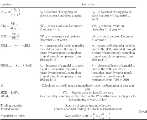
Table IIsums up the procedures used to calculate the variables analyzed in this study. The models described in Section 3.2 were estimated for the 1996-2005 period. The explanatory variables were measured by taking the dependent variable as a basis – stock return – measured between July of yeartand June of the following year. This procedure was used for all the analyzed period, that is, 1996-1997 to 2014-2015.
The predictor variables for B/M (FBMt) and ROE (FROEt), for eachfirm, were obtained through a linear dynamic panel estimation (Arellanoet al., 1991). Our study used the data from variablesBMt 1andROEt 1for all samplefirms over the period of analysis (1995 to 2010) to estimate the prediction model of each variable. Next, this model was used to generate the forecasts for eachfirm individually, year after year, based on the data of yeart–1.
Table II. Variables analyzed in this study
Equation Description
Rt¼ln Pit Pit 1
Pit= Nominal closing price of stockiin yeart(adjusted to gain);
Pit 1= Nominal closing price of stockiin yeart 1 (adjusted to gain)
BMt¼ BVt 1
MVt 1
BVt 1= book value on December 31 of yeart 1;
VMt 1= market value on December 31 of yeart 1
ROEt¼NPt 1 BVt 1
NPt 1= company’s net profit on December 31 of yeart 1;
BVt 1= book value on December 31 of yeart 1
FBMtþ1=g0þg1BMt g0= intercept of a model to predict the B/M, estimated through a linear dynamic panel, using data from all sample companies, from 1995 to 2010;
g1= slope coefficient of a model to predict the B/M, estimated through a linear dynamic panel, using data from all sample companies, from 1995 to 2010
FROEtþ1=l0þl1ROEt l0= intercept of a model to predict the ROE, estimated through a linear dynamic panel, using data from all sample companies, from 1995 to 2010;
l1= slope coefficient of a model to predict the ROE, estimated through a linear dynamic panel, using data from all sample companies, from 1995 to 2010
bt Calculated on the 60 months immediately prior the beginning of yeart, in July
SIZEt= lnMVt VMt= Market value on June 30 of yeart
MOMt Calculated by summing up the return of the 12 months immediately prior to the beginning of yeart, in July
Trading quantity Quantity of annual trading of a stock Traded volume Volume of annual trading of a stock, in Brazilian Reais
4. Data analysis 4.1 Descriptive statistics
Table IIIshows the descriptive statistics of the analyzed variables. For most of the studied variables all the annual observations were valid (1691 observations). The average B/M was relatively low, if compared to its maximum value. According toFama and French (1993), low B/M ratios indicate growth opportunities. Beta and momentum had low variability levels. However, size and liquidity had a high variability. Three proxies were used to measure liquidity (trading quantity, traded volume and negotiability index), as liquidity cannot be directly observed, and it has several aspects that cannot be captured in a single measure (Liu, 2006).
The relations among the eight explanatory variables of this study were also investigated, through a correlation matrix (Table IV). As expected, the B/M ratio had a high positive correlation (0.751) with its predictor variable (FBM); a positive correlation was also found between the aggregate predictor variable (FRM) and the three fundamental variables that comprise it (B/M, FBM and FROE), corresponding to 0.957, 0.542 and 0.320, respectively. It is worth mentioning the positive correlation between size and the three proxies for liquidity (0.493, 0.585, 0.507, respectively), corroborating the results ofMachado and Medeiros (2011), who suggest that market value might be a reasonable proxy for liquidity. Finally, note the strong positive correlation between the three liquidity measures, which suggests that negotiability, trading quantity and traded volume may be capturing the same dimension as liquidity.
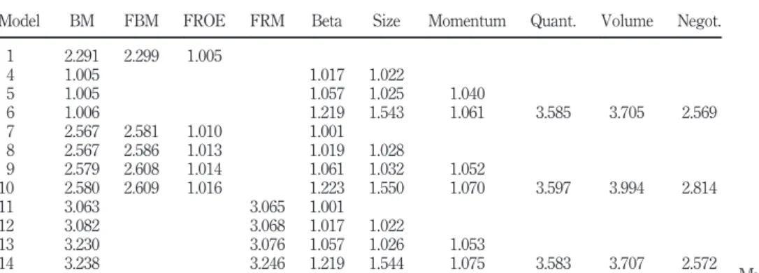
Considering the high correlation between some variables, as evidenced inTable IV, the authors found it was suitable to previously investigate a possible multicollinearity in the multivariate models. For this, the variance inflation factor test (VIF) was run for each explanatory variable. According to Levine et al. (2000), in case there is no correlation between a set of variables, the VIF will equal 1. In case the variables are highly correlated, the VIF may exceed 10. More conservative criteria suggest the presence of multicollinearity should the VIF exceed 5. The values found for the VIF test are inTable V.
The data inTable Vshow that, although not all the models had VIF test values around 1, none of them had a value over 5, considering a conservative analysis criterion. Therefore, the inexistence of collinearity across the explanatory variables may be confirmed. This finding ensures a more consistent use of multiple regression models; in this sense, the panel data estimation reduces the likelihood of multicollinearity problems.
Table III.
Descriptive statistics of the studied variables
Variable
No. of
observations Average SD Minimum Maximum
BM 1,691 3.4787 9.04 92.67 81.30
BM forecast 1,602 3.3170 2.94 23.24 30.08 ROE forecast 1,602 0.0957 0.02 0.25 0.36 Aggregate forecast
(FRM)
1,691 0.4269 7.32 80.43 64.36
Beta 1,339 0.7730 0.25 0.07 2.10
Size (in thousand R$) 1,688 5,592,396.33 20,413,196.54 376 286,390,438
Momentum 1,691 0.1125 0.47 2.10 2.76
Liquidity
Negotiability 1,691 0.4045 1.13 0.03 12.56 Trading quantity 1,691 146.748.55 615.960.03 6 8.114.196 Traded volume (R$) 1,691 2,922,968 14,937,630.12 14 218,327,039
Notes:The variables were calculated according to the procedures described inTable II. Size, trading
quantity and traded volume are shown in grossfigures. The remaining variables are indices
RAUSP
53,3
Finally, a stationarity test of the dependent variable (stock return) was run. We used the
Levinet al.(2002)test because it is a unit root test in panel data, developed with the intention to improve the explanatory power of conventional stationarity tests, for combining time and cross-section information. The unit root test results are inTable VIand show that all the variables are stationary at level, as the null hypothesis of the unit root was rejected.
4.2 Predictor variable estimations
The expected future B/M ratio and ROE were estimated through a linear dynamic panel of
Arellano et al. (1991), whose estimators are obtained through a Generalized Method of Moments (GMM). The study used the B/M ratio and ROE data of 89 stocks that comprised the sample for the whole period of analysis (1995 to 2015) to estimate the predictor models for each variable, considering the series stationarity (Table VI).Equation (8)has the predictor model for the B/M ratio andequation (9)has the predictor model for the ROE, both with a lag:
FBMtþ1¼2:078þ0:344BMt (8)
Table V. Multicollinearity test for the multivariate models Model BM FBM FROE FRM Beta Size Momentum Quant. Volume Negot.
1 2.291 2.299 1.005
4 1.005 1.017 1.022
5 1.005 1.057 1.025 1.040
6 1.006 1.219 1.543 1.061 3.585 3.705 2.569 7 2.567 2.581 1.010 1.001
8 2.567 2.586 1.013 1.019 1.028
9 2.579 2.608 1.014 1.061 1.032 1.052
10 2.580 2.609 1.016 1.223 1.550 1.070 3.597 3.994 2.814 11 3.063 3.065 1.001
12 3.082 3.068 1.017 1.022
13 3.230 3.076 1.057 1.026 1.053
14 3.238 3.246 1.219 1.544 1.075 3.583 3.707 2.572
Note:For each model described in regression models estimated in this study, a multicollinearity test was
run, the VIF test statistics values are presented above
Table IV. Correlation matrix of the explanatory variables BM FBM FROE FRM BETA SIZE MOM LIQ1 LIQ2 LIQ3
BM 1.000 0.751** 0.038 0.957** 0.007 0.062* 0.006 0.035 0.034 0.004 FBM 1.000 0.068** 0.542** 0.008 0.072** 0.054* 0.048 0.044 0.020 FROE 1.000 0.302** 0.027 0.054* 0.047 0.027 0.032 0.044 FRM 0.001 0.054* 0.018 0.030 0.029 0.003 BETA 1.000 0.128** 0.188** 0.195** 0.180** 0.338**
SIZE 1.000 0.025 0.493** 0.585** 0.507**
MOM 1.000 0.066** 0.037 0.013
LIQ1 1.000 0.843** 0.566**
LIQ2 1.000 0.734**
LIQ3 1.000
Notes: Proxies for liquidity: 1 = Trading quantity; 2 = Traded volume; 3 = Negotiability; *significant at
1%; **significant at 5%
Return on
equity and
Brazilian Stock
Returns
FROEtþ1¼0:938þ0:024ROEt (9) Next, these two models were used to generate the B/M ratio and ROE predictions for each firm individually, year after year, based on the data of yeart. The main contribution of this estimation method for the expected future B/M ratio and ROE is the fact that it allows for an autoregressive estimation model that takes in consideration the heterogeneity of the stocks offirms that comprise the sample. In addition, the use of the linear dynamic panel with data for the whole period of analysis (1995-2015) is believed to favor obtaining a predictor model that is valid for the whole period.
4.3 Analyzing the explanatory capacity of the models
This section aims to analyze the contribution of the analyzed variables to explain stock returns in the Brazilian market. For this, the study used panel data regressions across the annual stock returns and the two groups of explanatory variables.
To start with, we present the results of the models proposed byClubb and Naffi(2007), comprising fundamental variables. Next, we present the models comprising risk-factor approach variables. Finally, we analyze the models formed on combinations of these two groups of variables, as a robustness test for the results of previous phases.
4.3.1 Fundamental valuation models. Table VII shows the regression results for the fundamental valuation models. Model 1 constitutes the multivariate model proposed by
Clubb and Naffi(2007), comprising the B/M ratio and the expected future B/M and ROE. The coefficient of determination (R2) was 0.0287. In the study ofClubb and Naffi(2007), which used data from the UK from 1991 to 2000, this model’sR2was 0.0932. The coefficients of the three fundamental variables were consonant with the theoretical framework that the model requires, as described in Section 3.2.1. The coefficient for the B/M ratio was positive and significant at the 1 per cent level. The predictor variables of the B/M and ROE also had a sign consistent with expectations; however, they were not statistically significant. The coefficients found byClubb and Naffi(2007)for the B/M ratio at level and for the B/M ratio predictor variable were statistically significant at the 1 per cent level, and the coefficient for the ROE predictor variable was significant at the 5 per cent level.
Model 2, univariate, is formed by the aggregate predictor variable proposed byClubb and Naffi(2007): FRM:BMt–FBMtþ1þFROEtþ1. The coefficient of determination (R2)
Table VI. Stationarity test for panel data
Variable t-statistic p-value
Return 14.09* 0.0000
BM 7.84* 0.0000
BM forecast 4.53* 0.0000
ROE forecast 7.81* 0.0000
Aggregate forecast (FRM) 46.70* 0.0000
Beta 2.50* 0.0000
Size 1.80** 0.0353
Momentum 17.64* 0.0000
Liquidity
Negotiability 10.56* 0.0000
Trading quantity 17.29* 0.0000
Traded volume 6.86* 0.0000
Notes:*Significant at 1%; **significant at 5%
RAUSP
53,3
was 0.0452, representing a considerable improvement compared to Model 1. Comparatively,
Clubb and Naffi(2007)found a coefficient of determination of 0.0891 for this model. The coefficient of the FRM variable was significant at the 1 per cent level and the sign was consistent with that which was expected.Clubb and Naffi(2007)also found a positive and statistically significant coefficient for this variable.
The results of the regressions on the fundamental variables show that the explanatory power of the B/M ratio is not enhanced by the inclusion of expected future B/M ratio and ROE, considered separately, as these variables were not statistically significant. However, when the three variables are jointly taken, in the form of aggregate predictor variable, their explanatory power is superior to the B/M ratio when taken individually.
According toClubb and Naffi(2007), although the premises of the models imply that the explanatory power of both should be identical, possible distortions in measuring the predicted variables (FBMtþ1and FROEtþ1) may cause a difference in the explanatory power of Models 1 and 2. Therefore, the results found for the fundamental valuation suggest that the multivariate model proposed byClubb and Naffi(2007)is apparently not suitable for the Brazilian stock market and is not relevant to explain stock returns. On the other hand, the univariate model shows that, when combined with the B/M ratio, in the form of aggregate variable, the B/M ratio and ROE predictor variables are superior to the B/M ratio found in the study in terms of explanatory capacity of the stock returns.
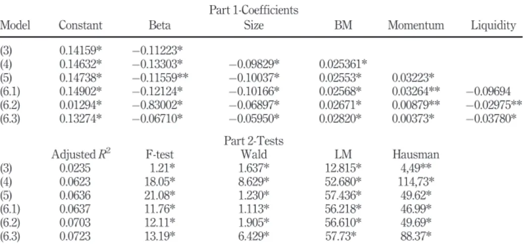
4.3.2 Risk-factor approach models. To compare the explanatory capacity of the fundamental variables presented in the previous section to the risk-factor approach variables, traditionally suggested in the literature, this section discusses the results of the regressions for the risk-factor approach models, which are shown inTable VIII. In general terms, the results confirm the importance of some of these variables and the existence of specific anomalies in the Brazilian stock market.
The beta coefficient was statistically significant in all the estimated models. However, it had a negative sign, contradicting the theoretical hypothesis that risk and return are directly proportional variables. In Brazil, Vieira and Milach (2008) found the same evidence. According to these authors, such result might suffer the influenced of the behavior of return over the studied period (1995-2005).
Considering that most of each stock returns had negative values and that each stock betas had positive values, when regressed, the beta coefficients were, on average, negative. Another Brazilian evidence of the negative relation between the beta and return was found
Table VII. Results of the fundamental valuation models’ regressions Part 1-Coefficients
Model Constant BM FBM FROE FRM
(1) 0.0400531* 0.07376* 0.035035 0.111385
(2) 0.0678418* 0.0180011*
Part 2-Tests
AdjustedR2 F-Test Wald LM Hausman
(1) 0.0287 3.88* 4.40* 6.66* 30.51*
(2) 0.0452 1.47* 3.13* 2.1900 10.99*
Notes: Part 1 of the Table shows fundamental valuation model regressions estimated annually through
panel data. The expected future B/M ratio (FBM) and ROE (FROE) were estimated through the linear dynamic panel ofArellanoet al.(1991). Standard errors were estimated using a Huber–White robust matrix, considering the results of the tests of regression assumptions, which are in Part 2 of the Table; *significant at 1%
Return on
equity and
Brazilian Stock
Returns
byCorreiaet al. (2008), who used data from 1995 to 2004. To these authors, this result suggests that the beta cannot reflect the effect expected from the systematic risk.Dataret al. (1998)also found negative betas when using data from the US market from 1962 to 1991. They underscore that measuring the beta depends on the efficiency of the proxy used for market portfolio and on the interval extent and measuring procedure adopted.
This study used the beta coefficient available from the Economatica database, calculated on a 60-month period prior to each year’s start date. The study found that a considerable part of the stocks had negative returns in the studied period (25.5 per cent), which comprehended the current worldfinancial crisis. So, we believe that the estimated beta coefficient may not represent the systematic risk or simply may not be reflecting a specific characteristic of the Brazilian market in the context under study. It is important to note that the main objective of this study is to assess the importance of the fundamental variables to explain the stock returns and that the beta is being used solely as a control variable.
Regarding the B/M ratio, the study found, in all models, a positive relation that was previously expected. The B/M was, therefore, an important variable to explain Brazilian stock returns. Thisfinding confirms classic evidence on the B/M effect, such as inChanet al. (1991),Fama and French (1992,1993),Capaulet al.(1993),Lakonishoket al.(1994).
Size did not present a statistically significant negative relation with return, which corroborates the classic evidence for size (Banz, 1981). Clubb and Naffi (2007) found a positive relation between size and return, though statistically insignificant in all risk-factor approach models.
Momentum had a positive coefficient, which corroborates the assumption found in the literature that there is a positive relation between momentum and the expected stock returns. However, there was no statistical significance in any of the estimated models. The momentum effect, proposed byJegadeesh and Titman (1993,2001), shows that the strategies to buy stocks that had good results in the past (Win) and sell stocks that had bad results in
Table VIII. Regression results for the risk-factor approach models
Part 1-Coefficients
Model Constant Beta Size BM Momentum Liquidity
(3) 0.14159* 0.11223*
(4) 0.14632* 0.13303* 0.09829* 0.025361*
(5) 0.14738* 0.11559** 0.10037* 0.02553* 0.03223*
(6.1) 0.14902* 0.12124* 0.10166* 0.02568* 0.03264** 0.09694 (6.2) 0.01294* 0.83002* 0.06897* 0.02671* 0.00879** 0.02975** (6.3) 0.13274* 0.06710* 0.05950* 0.02820* 0.00373* 0.03780*
Part 2-Tests
AdjustedR2 F-test Wald LM Hausman (3) 0.0235 1.21* 1.637* 12.815* 4,49** (4) 0.0623 18.05* 8.629* 52.680* 114,73* (5) 0.0636 21.08* 1.230* 57.436* 49.62* (6.1) 0.0637 11.76* 1.113* 56.218* 46.99* (6.2) 0.0703 12.11* 1.905* 56.610* 49.69* (6.3) 0.0723 13.19* 6.429* 57.73* 88.37*
Notes: Part 1 of the Table shows the regression results for the risk-factor approach models estimated
annually through panel data. Standard errors were estimated using a Huber–White robust matrix, considering the results of the tests of regression assumptions, which are in Part 2 of the Table, 1 = Negotiability, 2 = Trading quantity, 3 = Traded volume; *significant at 1%; **significant at 5%; and *** significant at 10%
RAUSP
53,3
the same period (Los) generate significantly positive returns over the following months.
Carhart (1997)considered momentum a risk factor, which led to the four-factor model. Finally, we found the existence of a liquidity premium in the Brazilian market, as the three proxies used had a negative relation with return, trending quantity and traded volume were statistically significant. This result ratifies thefindings of Machado and Medeiros (2012)in the Brazilian market and those ofAmihud and Mendelson (1986),Liu (2006)and
Keene and Peterson (2007)in the USA. In addition, the explanatory power of the said models was very close, thus confirming the evidence raised in Section 4.1, that the three measures may be capturing the same dimension as liquidity.
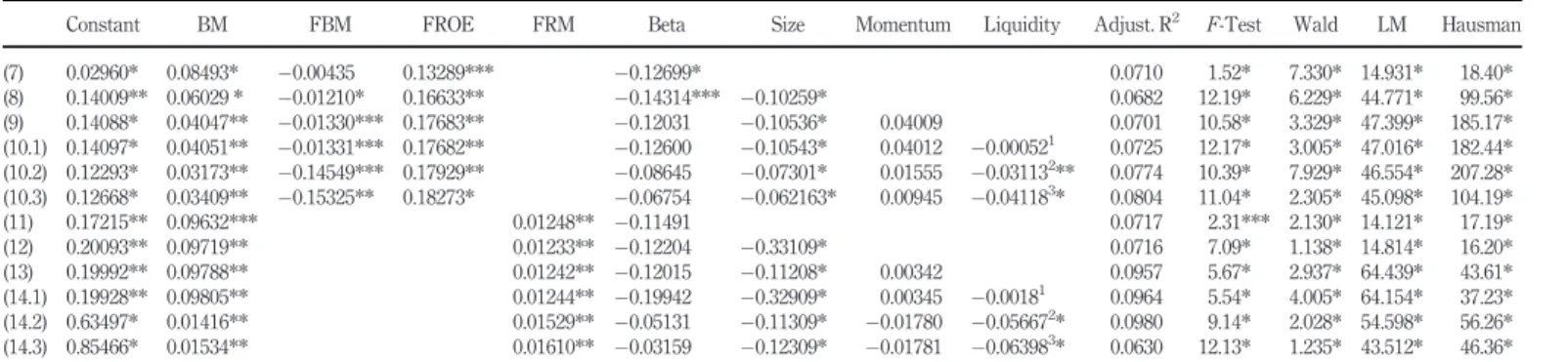
4.3.3 Robustness tests–joint models.In this section, we discuss the results of the joint
model regressions, which combine the variables of the two approaches described above. The results found in this step were slightly different from the evidence presented in the previous steps.Table VIIshows that B/M and ROE predictor variables did not have explanatory power for stock returns, when taken separately. However, in the joint model regressions, the expected future ROE (FROE) had statistical significance in all models and the expected future B/M ratio was significant in Models 8 to 10. Both presented the expected sign. The analysis of the models’coefficient of determination (adjustedR2) shows that, in joint models, the explanatory capacity of the stock returns was enhanced, both in relation to the fundamental valuation models and to those formed by the risk factors, when considered separately. This result ratifies thefindings ofClubb and Naffi(2007), in that the explanatory power of the models was enhanced by the B/M and ROE predictor variables.
The results found with the joint models that included the aggregate predictor variable (FRM) show that it remained consistent after the inclusion of all the risk-factor approach variables. In addition, the coefficients of determination of these models were superior to those found in the fundamental valuation models and risk-factor approach, separately. This result reinforces the evidence shown inTable VIII, which indicates the contribution of such variable to explain Brazilian stock returns.
The control variables were found to keep presenting the same relations as those shown in
Table VIII. However, the beta had statistical significance only in Models 7 and 8, and momentum was not significant to explain the analyzed stock returns, after combined with the fundamental variables. The control variables that remained consistent across this phase were size and two liquidity proxies: trading quantity and traded volume.
Finally, all the analyzed models in this work were estimated again, using the period from 1995 to 2007, to verify whether they were being influenced by the worldfinancial crisis, started in 2008. In general, there were no substantial changes in the results found. Because of space constraints, the results of such estimations were not presented in this paper, but they can be provided upon request to the authors.
Summing up, the results found show that the joint models (Table IX) had and explanatory power superior to the models of the two approaches, when taken separately. This result was also found by Clubb and Naffi (2007). This way, both the fundamental valuation and the risk-factor approach are important to explain stock returns in Brazil. Considering the coefficient of determination (R2), the model that had the best explanatory power, when future expectations were taken separately, was 10.3.
Considering the aggregate predictor variable FRM, the model that had the best explanatory capacity was 14.2. Finally, it is worth mentioning the importance of the B/M ratio as an explanatory variable. The results found in this study show that the B/M has an explanatory capacity when combined with the expected future B/M and ROE, as an aggregate predictor variable and also as a risk factor.
Return on
equity and
Brazilian Stock
Returns
Constant BM FBM FROE FRM Beta Size Momentum Liquidity Adjust. R2 F-Test Wald LM Hausman
(7) 0.02960* 0.08493* 0.00435 0.13289*** 0.12699* 0.0710 1.52* 7.330* 14.931* 18.40*
(8) 0.14009** 0.06029 * 0.01210* 0.16633** 0.14314*** 0.10259* 0.0682 12.19* 6.229* 44.771* 99.56*
(9) 0.14088* 0.04047** 0.01330*** 0.17683** 0.12031 0.10536* 0.04009 0.0701 10.58* 3.329* 47.399* 185.17*
(10.1) 0.14097* 0.04051** 0.01331*** 0.17682** 0.12600 0.10543* 0.04012 0.000521 0.0725 12.17* 3.005* 47.016* 182.44*
(10.2) 0.12293* 0.03173** 0.14549*** 0.17929** 0.08645 0.07301* 0.01555 0.031132** 0.0774 10.39* 7.929* 46.554* 207.28*
(10.3) 0.12668* 0.03409** 0.15325** 0.18273* 0.06754 0.062163* 0.00945 0.041183* 0.0804 11.04* 2.305* 45.098* 104.19*
(11) 0.17215** 0.09632*** 0.01248** 0.11491 0.0717 2.31*** 2.130* 14.121* 17.19*
(12) 0.20093** 0.09719** 0.01233** 0.12204 0.33109* 0.0716 7.09* 1.138* 14.814* 16.20*
(13) 0.19992** 0.09788** 0.01242** 0.12015 0.11208* 0.00342 0.0957 5.67* 2.937* 64.439* 43.61*
(14.1) 0.19928** 0.09805** 0.01244** 0.19942 0.32909* 0.00345 0.00181 0.0964 5.54* 4.005* 64.154* 37.23*
(14.2) 0.63497* 0.01416** 0.01529** 0.05131 0.11309* 0.01780 0.056672* 0.0980 9.14* 2.028* 54.598* 56.26*
(14.3) 0.85466* 0.01534** 0.01610** 0.03159 0.12309* 0.01781 0.063983* 0.0630 12.13* 1.235* 43.512* 46.36*
Notes: Part 1 of the Table shows the regression results of the joint models estimated annually. The expected future B/M ratio (FBM) and ROE (FROE) were estimated through the linear dynamic panel ofArellanoet al.(1991). Standard errors were estimated using the Huber–White robust matrix, considering the results of the tests of regression assumptions, which are in Part 2 of the Table. 1 = Negotiability, 2 = Trading quantity, 3 = Traded volume; *significant at 1%; **significant at 5% and ***significant at 10%
Table
IX.
Regression
results
of
the
joint
models
RAUSP
53,3
5. Conclusion
This paper aimed to study the influence of expected future B/M ratio and ROE on explaining Brazilian stock market returns. The study concluded that the estimated future B/M ratio and ROE do not show statistical significance in the multifactor model proposed byClubb and Naffi(2007). However, when combined with the risk-factor approach variables, the predictor variables turn out to be significant and enhance the explanatory capacity of the models formed only by risk-factor approach variables.
The expected future B/M and ROE were also combined with the B/M ratio at level, forming an aggregate predictor variable. This variable was found to be statistically significant, both in the univariate model proposed byClubb and Naffi(2007)and after the inclusion offive control variables. In addition, the explanatory capacity of the models that included such variable was very superior to that obtained with the risk-factor approach regressions. Therefore, this paper’s initial hypotheses, that the expected future B/M ratio and the expected ROE explain part of the Brazilian stock return variations, cannot be rejected.
In this study, the B/M ratio was tested as a fundamental variable and with the risk-factor approach models. The findings show that the B/M ratio was positive and statistically significant in both classes of models. In addition, when inserted in the joint models, the study found the contribution of the expected future B/M, as a component of the aggregate predictor variable, as well as its additional explanatory capacity as a control variable.
In summary, the results found in this study indicate that the expected future B/M ratio and ROE, as well as an aggregate predictor variable, comprising the B/M ratio and the expected future B/M and expected ROE, influence the explanation of Brazilian stock returns. This means that these variables may be used in investment strategies in the stock market, because the B/M ratio plus the expected future B/M and ROE for the following year were capable of explaining part of the stock return variations in the same period. In addition, when combined withfirm size and liquidity, the expected future B/M and ROE were also capable of explaining part of Brazilian stock returns.
The main contribution of this study to the literature is to demonstrate how the expected future B/M ratio and ROE may improve the explanatory capacity of the stock return, when compared with the variables traditionally studied in the literature. This study found special characteristics of the Brazilian stock market which do not match the assumptions of the asset pricing theories or the evidences indicated in the literature, especially those of developed countries. Therefore, alternative perspectives to analyze market anomalies, such as fundamental valuation, herein focused, are suitable.
The evidences herein presented can also contribute to establishing investment strategies, considering that the B/M ratio may be calculated through accounting information announced by companies. Besides, using historical data enables investors, in a specific year, to calculate the predictor variables for the B/M ratio and ROE in the next year, which enhance the explanatory power of the current B/M, when combined in the form of an aggregate predictor variable for stock returns.
Still, it is important to mention that this research was limited to the non-financial companies with shares traded at the B3, from January 1, 1995 to June 30, 2015. This way, the conclusions reached are limited to the sample used herein. In addition, excluding the companies with a negative market value and low liquidity to obtain proxies of variables of this study may lead to a sample of liquid,financially-healthfulfirms.
As this is afield that has not been very explored in Brazil, the study on fundamental valuation and stock return opens alternatives to develop future research studies. This study used annual data and a dynamic panel method to estimate the predictor variables. This way,
Return on
equity and
Brazilian Stock
Returns
we suggest measuring the data with other bases, such as quarterly, for example, as well as using other methods to estimate the predictor variables. Another alternative is to carry out a comparative analysis per economic sector to confront the results herein presented.
References
Almeida, J.R. and Eid, W. Jr (2010),“Estimando o retorno das ações com decomposição do índice book-to-market: Evidências na bovespa”,Revista Brasileira de Finanças, Vol. 8 No. 4, pp. 417-441. Amihud, Y. and Mendelson, H. (1986),“Asset pricing and the bid-ask spread”,Journal of Financial
Economics, Vol. 17 No. 2, pp. 223-249.
Arellano, M., Bond, S., Url, S., Review, T., Studies, E. and Archive, T.J. (1991), “Some tests of specification for panel data: Monte Carlo evidence and an application to employment equations”,
The Review of Economic Studies, Vol. 58 No. 2, pp. 277-297.
Baltagi, B.H. (2005),Econometric Analysis of Panel Data, John Wiley, Chichester.
Banz, R.W. (1981),“The relationship between return and market value of common stocks”,Journal of Financial Economics, Vol. 9 No. 1, pp. 3-18.
Beaver, W.H. and Ryan, S.G. (2000),“Biases and lags in book value and their effects on the ability of the book-to-market ratio to predict book return on equity”,Journal of Accounting Research, Vol. 38 No. 1, pp. 127-148.
Berk, J. (1995),“A critique of size-related anomalies”,Review of Financial Studies, Vol. 8 No. 2, pp. 275-286.
Berk, J. (1997),“Does size really matter?”,Financial Analyst Journal, Vol. 53 No. 5, pp. 12-18.
Billings, B.K. and Morton, R.M. (2001),“Book-to-market components, future security returns, and errors in expected future earnings”,Journal of Accounting Research, Vol. 39 No. 2, pp. 197-219. Black, F. (1972),“Capital market equilibrium with restricted borrowing”,The Journal of Business,
Vol. 45 No. 3, pp. 444-455.
Capaul, C., Rowley, I. and Sharpe, W.F. (1993),“International value and growth stock returns”,
Financial Analysts Journal, Vol. 49 No. 1, pp. 27-36.
Carhart, M. (1997),“On persistence of mutual fund performance”,Journal of Finance, Vol. 52 No. 1, pp. 57-82.
Chan, L.K.C., Hamao, Y. and Lakonishok, J. (1991),“Fundamentals and stock returns in Japan”,The Journal of Finance, Vol. 46 No. 5, pp. 1739-1764.
Chen, L. and Zhao, X. (2006),“On the relation between the market-to-book ratio, growth opportunity, and leverage ratio”,Finance Research Letters, Vol. 3 No. 4, pp. 253-266.
Clubb, C. and Naffi, M. (2007),“The usefulness of book-to-market and ROE expectations for explaining UK stock returns”,Journal of Business Finance & Accounting, Vol. 34 Nos 1/2, pp. 1-32.
Correia, L.F., Amaral, H.F. and Bressan, A.A. (2008),“O efeito da liquidez sobre a rentabilidade de mercado das ações negociadas no mercado acionário brasileiro”,Revista de Administração E Contabilidade Da UNISINOS, Vol. 5 No. 2, pp. 109-119.
Datar, V.T., Naik, Y.N. and Radcliffe, R. (1998),“Liquidity and stock returns: an alternative test”,
Journal of Financial Markets, Vol. 1 No. 2, pp. 203-219.
Dorantes, C.D. (2013),“The relevance of using accounting fundamentals in the Mexican stock market”,
Journal of Economics, Finance and Administrative Science, Vol. 18, pp. 2-10.
Evrard, H.S., Cruz, J.A.W. and Da Silva, W.V. (2015),“Multifatorialidade e o retorno de ações brasileiras entre o período de 2003 e 2013”,Revista de Gestão, Finanças e Contabilidade, Vol. 5 No. 3, pp. 42-60.
Fairfield, P.M. (1994),“P/E, P/B and the present value of future dividends”,Financial Analysts Journal, Vol. 50 No. 4, pp. 23-31.
RAUSP
53,3
Fama, E.F. and French, K.R. (1992),“The cross-section of expected stock returns”,Journal of Finance, Vol. 47 No. 2, pp. 427-465.
Fama, E.F. and French, K.R. (1993),“Common risk factors in the returns on stocks and bonds”,Journal of Financial Economics, Vol. 33 No. 1, pp. 3-56.
Fama, E.F. and French, K.R. (2008),“Average returns, BM, and share issues”,The Journal of Finance, Vol. 63 No. 6, pp. 2971-2995.
Frankel, R. and Lee, C.M.C. (1998),“Accounting valuation, market expectation, and cross-sectional stock returns”,Journal of Accounting and Economics, Vol. 25 No. 3, pp. 283-319.
Hausman, J.A. (1978),“Specification tests in econometrics”,Econometrica, Vol. 46 No. 6, pp. 1251-1271. Jegadeesh, N. and Titman, S. (1993),“Returns to buying winners and selling losers: implications for
stock market efficiency”,The Journal of Finance, Vol. 48 No. 1, p. 65.
Jegadeesh, N. and Titman, S. (2001), “Profitability of momentum strategiesf: an evaluation of alternative explanations”,The Journal of Finance, Vol. 56 No. 2, pp. 699-720.
Keene, M.A. and Peterson, D.R. (2007),“The importance of liquidity as a factor in asset pricing”,Journal of Financial Research, Vol. 30 No. 1, pp. 91-109.
Kothari, S.P. (2001),“Capital markets research in accounting”,Journal of Accounting and Economics, Vol. 31 Nos 1/3, pp. 105-231.
Lakonishok, J., Shleifer, A. and Vishny, R.W. (1994),“Contrarian investment, extrapolation, and risk”,
The Journal of Finance, Vol. 49 No. 5, pp. 1541-1578.
Lee, C. (2001),“Market efficiency and accounting research: a discussion of‘Capital market research in accounting’by S.P. Kothari”,Journal of Accounting and Economics, Vol. 31 Nos 1/3, pp. 233-253. Lee, W.J. and Zhang, Y. (2014),“Accounting valuation and cross sectional stock returns in China”,
China Accounting and Finance Review, Vol. 16 No. 2, pp. 155-169.
Lev, B. and Sougiannis, T. (1999),“Penetrating the book-to-market black box: the R&D effect”,Journal of Business Finance and Accounting, Vol. 26 Nos 3/4, pp. 419-449.
Levin, A., Lin, C.F. and Chu, C.S. (2002),“Unit root test in panel data: asymptotic andfinite sample properties”,Journal of Econometrics, Vol. 108 No. 1, pp. 1-24.
Levine, D.M., Berenson, M.L. and Stephan, D. (2000),Estatística: teoria e Aplicações, LTC, Rio de Janeiro.
Lintner, J. (1965),“The valuation of risk assets and the selection of risky investments in stock portfolios and capital budgets”,The Review of Economics and Statistics, Vol. 47 No. 1, pp. 13-37.
Liu, W. (2006),“A liquidity-augmented capital asset pricing model”,Journal of Financial Economics, Vol. 82 No. 3, pp. 631-671.
Machado, M.A.V. and Medeiros, O.R. (2011),“Asset pricing models e o efeito liquidez: evidências empíricas no mercado acionário brasileiro”,Revista Brasileira de Finanças, Vol. 9, pp. 383-412. Machado, M.A.V. and Medeiros, O.R. (2012),“Existe o efeito liquidez no mercado acionário Brasileiro?”,
Brazilian Business Review, Vol. 9 No. 4.
Pontiff, J. and Schall, L.D. (1998),“Book-to-market ratios as predictors of market returns”,Journal of Financial Economics, Vol. 49 No. 2, pp. 141-160.
Richardson, S., Tuna, I. and Wysocki, P. (2010),“Accounting anomalies and fundamental analysis: a review of recent research advances”,Journal of Accounting and Economics, Vol. 50 Nos 2/3, pp. 410-454. Ryan, S.G. (1995),“A model of accrual measurement with implications for the evolution of the
book-to-market ratio”,Journal of Accounting Research, Vol. 33 No. 1, pp. 95-128.
Schwert, G. (2003),“Anomalies and market efficiency”, in Constatinides, G.., Harris, M.. and Stulz, R.M. (Eds),Handbook of the Economics of Finance, Vol. 15, North-Holland, Amsterdam, 937-972. Sharpe, W.F. (1963),“A simplified model for portfolio analysis”,Management Science, Vol. 9 No. 2,
pp. 277-293.
Return on
equity and
Brazilian Stock
Returns
Sharpe, W.F. (1964),“Capital asset prices: a theory of market equilibrium under conditions of risk”,
Journal of Finance, Vol. 19 No. 3, pp. 425-442.
Skogsvik, S. and Skogsvik, K. (2010),“Accounting-based probabilistic prediction of ROE, the residual income valuation model and the assessment of mispricing in the Swedish stock market”,Abacus, Vol. 46 No. 4, pp. 387-418.
Vieira, K.M. and Milach, F.T. (2008),“Liquidez/iliquidez no mercado brasileiro: comportamento no período 1995-2005 e suas relações com o retorno”,Revista De Administração e Contabilidade Da Unisinos, Vol. 5 No. 2, pp. 5-16.
Vuolteenaho, T. (2002),“What drives frim-level stock returns?”,Journal of Finance, Vol. 57 No. 1, pp. 233-264.
RAUSP
53,3
Appendix
Company Sector Share Share class
Alfa Consorcio Other BRGE11 PNE
Alfa Consorcio Other BRGE12 PNF
Alfa Consorcio Other BRGE3 ON
Alfa Holding Other RPAD3 ON
Alfa Holding Other RPAD5 PNA
Alfa Holding Other RPAD6 PNB
Alpargatas Textile ALPA3 ON
Alpargatas Textile ALPA4 PN
Ambev Food and Beverage AMBV3 ON
Ambev Food and Beverage AMBV4 PN
Ampla Energia Electricity CBEE3 ON
Bardella Industrial machinery BDLL4 PN
Bombril Chemical industry BOBR4 PN
Brasil Telecom Telecommunications BRTO3 ON Brasil Telecom Telecommunications BRTO4 PN
Braskem Chemical industry BRKM5 PNA
Brasmotor Electronics BMTO4 PN
CELESC Electricity CLSC6 PNB
CEMIG Electricity CMIG3 ON
CEMIG Electricity CMIG4 PN
CESP Electricity CESP3 ON
CESP Electricity CESP5 PNA
CONFAB Steelmaking and Metallurgy CNFB4 PN
COPERL Electricity CPLE3 ON
Coteminas Textile CTNM3 ON
Coteminas Textile CTNM4 PN
Panvel Farmácias Commerce PNVL3 ON
Panvel Farmácias Commerce PNVL4 PN
Eletrobrás Electricity ELET3 ON
Eletrobrás Electricity ELET6 PNB
Estrela Other ESTR4 PN
Eternit Non-Metallic Minerals ETER3 ON Ferbasa Steelmaking and Metallurgy FESA4 PN Forjas Taurus Steelmaking and Metallurgy FJTA4 PN
Fras-Le Vehicles and parts FRAS4 PN
Gerdau Steelmaking and Metallurgy GGBR3 ON Gerdau Steelmaking and Metallurgy GGBR4 PN Gerdau Metalúrgica Steelmaking and Metallurgy GOAU4 PN
Inepar Other INEP4 PN
Itaúsa Other ITSA3 ON
Itaúsa Other ITSA4 PN
Itautec Philco Electronics ITEC3 ON
Klabin S/A Paper and Cellulose KLBN4 PN
Light S/A Electricity LIGT3 ON
Lojas Americanas Commerce LAME4 PN
M G Poliest Chemical industry RHDS3 ON (continued)
Table AI. Stocks that comprise the research sample
Return on
equity and
Brazilian Stock
Returns
*Corresponding author
Rebeca Cordeiro da Cunha Araújo can be contacted at:[email protected]
For instructions on how to order reprints of this article, please visit our website:
www.emeraldgrouppublishing.com/licensing/reprints.htm
Or contact us for further details:[email protected]
Company Sector Share Share class
Mangels Indl Steelmaking and Metallurgy MGEL4 PN
Marcopolo Vehicles and parts POMO4 PN
Metisa Steelmaking and Metallurgy MTSA4 PN
Petrobras Petrol and Gas PETR3 ON
Petrobras Petrol and Gas PETR4 PN
Pettenati Textile PTNT4 PN
Pro Metalurg Vehicles and parts PMET6 PNB Randon Participações Vehicles and parts RAPT4 PN
Recrusul Vehicles and parts RCSL4 PN
Sansuy Indústria de Plásticos Other SNSY5 PNA Companhia Siderúrgica Nacional Steelmaking and Metallurgy CSNA3 ON
Souza Cruz Other CRUZ3 ON
Construtora Sultepa Construction SULT4 PN Suzano Papel Paper and Cellulose SUZB5 PNA
Teka Textile TEKA4 PN
Telemar Telecommunications TMAR3 ON
Telesp Telecommunications TLPP3 ON
Telesp Telecommunications TLPP4 PN
Unipar Participações Chemical industry UNIP6 PNB Usiminas Steelmaking and Metallurgy USIM3 ON Usiminas Steelmaking and Metallurgy USIM5 PNA
Vale Mining VALE3 ON
Vale Mining VALE5 PNA
Valefert Chemical industry FFTL4 PN
Wetzel S/A Vehicles and parts MWET4 PN
Whirlpool Electronics WHRL4 PN
Wlm Indústria e Comércio Commerce SGAS4 PN Yara Brasil Fertilizantes Chemical industry ILMD4 PN Table AI.