A Work Project, presented as part of the requirements for the Award of a Master Degree in Finance from the NOVA – School of Business and Economics
FINANCIAL STATEMENT INFORMATION FOR VOLATILITY ESTIMATION
JOÃO ALBUQUERQUE DA CRUZ ALVES | 860
A Project carried out under the supervision of Professor Paulo M. M. Rodrigues
2 FINANCIAL STATEMENT INFORMATION FOR VOLATILITY ESTIMATION
Abstract
This work extends Sridharan’s (2015) results, who found a significant relationship between financial variables and realized volatility. In particular, the introduction of Size, Research and Development Expenditures, Sales Growth, Cash Flow Volatility, Earnings
Opacity, Leverage, Return on Assets and Equity Book-to-Market Ratio in a model based
on the volatility implied in option market prices presented improved results. Applying a similar methodology to a different set of data, it is found that only three of those variables affect realized volatility in my sample. Leverage and Equity Book-to-Market Ratio have a negative impact and Return on Assets a positive impact. It is hypothesized that financial variables should also be useful in the construction of a traditional ARCH model. This is confirmed empirically and it is shown that the better volatility forecasts, provided by the introduction of these financial variables, can be used to construct a successful investment strategy that outperforms the market.
Keywords:
3 I. Introduction
Eugene Fama (1970), in his influential article “Efficient Capital Markets”, termed as efficient a market in which prices always ‘fully reflect’ available information and this became known as EMH (Efficient Market Hypothesis). A semi-strong form of this EMH implies that all publicly available information is already incorporated in prices and, consequently, it is not possible to detect mispriced securities and design a profitable investment strategy using information such as financial statement figures. Despite the widely acceptance and ‘intellectual dominance’ of the efficient-market revolution (Malkiel, 2003), a counterrevolution is going on, conducted by fundamental analysts, who believe it is possible that, in the short run, the market misprices securities, and by econometricians, who argue that stock returns are, to a considerable extent, predictable.
The discussion, arguments and results about the efficiency of the market are not very relevant for this dissertation. What is important to highlight is that the current literature presents a wide range of studies incorporating financial statement information in the prediction of returns, such as Caneghem, et al, (2002), Alexakis, et al, (2010) and Goslim, et al, (2012). By contrast, however, regarding volatility estimation, the existing models
are much more closed and leave out most of the information about the firms which is usually considered in returns modeling. I believe that there are, at least, two reasons for this. First, the specific characteristics of financial data, namely the evidence of volatility clustering, low decay correlations, volatility persistence and ‘leverage’ effects have
4 σ𝑖,𝑅𝑉𝑡+𝜏 = β0 + β1σ𝑖,𝐼𝑉𝑡,𝜏 + β2 Year + ε𝑖,𝑡 (1) where σ𝑖,𝑅𝑉𝑡+𝜏 stands for realized volatility of firm i between t and 𝑡 + 𝜏; σ𝑖,𝐼𝑉𝑡,𝜏 stands for the implied volatility of firm i between t and 𝑡 + 𝜏 and Year is a vector of year fixed effects, with some authors showing that implied volatility for an at-the-money option is an unbiased estimator for the average volatility over the remaining life of the option (Christensen and Strunk, 2002).
Among all these models and contrasting to what is found in the returns literature, financial statement information was, surprisingly, never hypothesized to be relevant for the explanation of volatility. An original study conducted by Sridharan (2015) tested the usefulness of adding financial information into a volatility model, similar to that in equation (1), but controlling for past volatility, σ 𝑅𝑉
𝑖,𝑡−1, and liquidity, Spread, resulting in
(2)
σ𝑖,𝑅𝑉𝑡+𝜏 = β0 + β1σ𝑖,𝐼𝑉𝑡,𝜏 + β2V_FSV𝑖,𝑗𝑡 + β3 𝑆𝑝𝑟𝑒𝑎𝑑𝑖𝑡 + β4 σ𝑖,𝑡−1𝑅𝑉 + β5 Year + ε𝑖,𝑡 (2) where V_FSV𝑖,𝑗𝑡, represents a set of financial statement variables that were separately included in the equation.
Considering the logical assumption that a fully efficient option market would imply β1 not statistically different from one and β2 not statistically different from zero, Sridharan (2015) verifies in her empirical analysis that some financial variables are able to provide additional information to the market expectations about future volatility reflected in options prices. The obtained results were important in the sense they attested implied volatility as a biased estimator of future realized volatility, but especially because they revealed the importance of fundamental variables for volatility estimation.
5 of this nature, because options on a certain stock are not always available. Analyzing worldwide stocks, one realizes about the existence of many companies which, despite having equity shares publicly traded on a stock exchange, do not have marketed stock options. The main reason for this, is the fact that some companies do not have enough dimension to assure liquidity in derivative instruments. Also, it is unusual to find a highly developed derivatives industry, such as in America and Asia. Still, one may find it necessary to estimate returns volatility on a stock without options. Some examples may be highlighted: risk management purposes, evaluation of portfolio performance, determination of option prices in a first stock option issue.... In these cases, the use of a traditional volatility model is required1.
My goal is to extend Sridharan’s (2015) results, by analyzing whether accounting information can also be used in the construction of a traditional ARCH family volatility model. I use a different set of data (medium European companies, instead of big American companies), which also contributes to extend the results to another geographical area and to companies with different fundamental characteristics. In addition, I also intend to evaluate an investment strategy based on the results obtained. My research is divided in five parts. The next section discusses relevant literature for my analysis, section III describes the sample used, section IV presents the methodological design of the study, section V shows the results obtained and finally, in section VI, some conclusions are drawn.
II. Literature Review
As previously mentioned, Sridharan (2015) was the first study considering the hypothesis of using financial statement information for volatility estimation. The study
6 was initially published as a working paper, in 2012, and obtained good academic acceptance. For example, in a similar study, Goodman, Neamtiu and Zhang (2013), using data from different companies and testing a different set of financial variables, confirmed that information about a firm’s fundamental volatility is not fully priced in option contracts. Moreover, in the second edition of the book “Volatility Trading”, Sinclair (2013, Chapter 4.5), presents a summary of Sridharan’s results to teach the importance of fundamental information in volatility forecasting.
In the first part of my research I will follow the methodology used by this author. Therefore, it will be useful to describe in more detail some aspects of the referred paper. A sample comprising 1,126 firms with quarterly observations during 14 years of data was used to test two hypothesis. The first was that financial variables are related with future equity returns volatility and the second was that options markets are not fully efficient. As explained in the previous section, I do not intend to explore the discussion about the options market efficiency and, so, I will only focus on the results obtained by testing the first hypothesis. The following model was considered,
σ𝑖,𝑅𝑉𝑡+𝜏 = β0 + β1V_FSV𝑗
𝑖,𝑡 + β2 Year + ε𝑖,𝑡 (3)
where V_FSV represents eight fundamental variables considered to be potentially relevant to affect realized volatility: Size; Research and Development Expenditures; Sales Growth; Cash Flow Volatility; Earnings Opacity; Leverage; Returns on Assets; and
Equity Book-to-Market Ratio. Each variable showed evidence to be related with realized
volatility, as the coefficients were all significant at a 1 percent significance level. Size and Return on Assets were negatively related with the dependent variable, while the remaining
7 variables similar to those. In the next subsection, I review the literature that justifies why these specific eight variables are apparently related with volatility.
II.1 Financial Statements and Volatility
Although the referred study was original directly relating fundamentals with volatility estimation, prior literature had already documented significant relations between financial information and measures of risk or uncertainty, such as default risk, the incidence of extreme returns and growth opportunities. In its most basic financial definition, volatility is also a measure of risk or uncertainty and, therefore, we can suppose that a factor related with default risk, for instance, is also likely to affect volatility. Following this reasoning: Size – With mixed results there is some literature relating default risk with firm size.
For example, Bonfim (2007) notes that firms in default tend to be slightly bigger firms, but Eklund et al (2001) estimated a negative relationship between default probability and firm size, as measured by total assets. However, larger firms are less likely to report earnings surprises (Barton and Simko, 2002) and have a lower probability of becoming a target of a merger or acquisition (Palepu, 1986). Size is, therefore, expected to be negatively related with volatility.
8 volatility. Although the authors had verified this relationship, they did not develop a model for volatility estimation, neither went further investigating the relationship between other financial variables and returns volatility. The reason why I use personal expenses to assets instead of R&D expenses is that most of the firms in the sample do not report R&D in their statements. Nevertheless, it is plausible to assume that personal expenses and R&D expenses are positively related, since the variation of both might represent an investment or disinvestment pursuit by a firm.
Sales Growth – Sales Growth can also be considered as an indicator of growth opportunities and, therefore, the same reasoning used for R&D expenditures can be applied. Moreover, Baneish (1999) shows that higher sales growth may be indicative of a higher probability of earnings manipulation and Sun (2009) notes that the suspicion of manipulation and anticipation of restatements increases uncertainty and hence volatility. I expect sales growth to be positively related with returns volatility.
Cash Flow Volatility – Corporate risk management theory indicates that cash flows
volatility is negatively valued by investors. One reason for this is revealed by Minton and Schrand (1999), who empirically showed that higher cash flow volatility not only increases the likelihood that a firm will need to access capital markets, but also increases the costs of doing so. Consistent with that, Allayannis and Weston (2005) estimate that one standard deviation increase in cash flow volatility should result in a decrease in the firm value between 0 and 14 percent. Considering that portfolios composed by firms with lower market capitalization tend to have higher volatility than portfolios of firms with higher market capitalization (Fama and French, 2008), I expect cash flows volatility to be positively related with equity volatility.
9 opacity indicates less disclosure of firm-specific information, which suggests higher probability of managed earnings. Moreover, they show that more opaque firms are more likely to experience stock price crashes. I expect a positive relationship between earnings opacity and returns volatility.
Leverage – Some literature established a link between leverage levels and probability
of default. Hui, Lo and Huang (2007), Beaver (1966) and Kaplan and Gabriel (1979) all show a positive relationship between those two variables. Considering that default probability increases uncertainty about future returns, it should increase volatility as well. I expect returns volatility to increase with a firm’s leverage.
Returns on Assets – Along with leverage, another financial ratio commonly used in
predictive default models is the return on assets (ROA), a profitability measure. Maricia and Vintila (2012) and Beaver (1966), for instance, present a negative correlation between ROA and default probability. A potential reason is that capital markets are concerned about a firm’s ability to repay its debt and profitability is an important indicator of that
(Beaver, McNichols and Rhie 2005). In opposition to leverage, I expect ROA to be negatively related with returns volatility.
Equity Book-to-Market Ratio – Some studies, such as Fama-French (1994), suggest
10 II.2 Volatility Estimation
When modeling financial market volatility, one must consider several salient features that financial time series usually present, known as stylized facts. These include fat tail distributions of risky asset returns, asymmetry and mean reversion, co-movements of volatilities across assets and financial markets (Poon and Granger, 2003) and the fact that price changes are not independent over time, firstly documented by Mandelbrot (1963, p.418), who noted that “large changes tend to be followed by large changes – of either sign – and small changes tend to be followed by small changes”, a phenomenon known as ‘volatility clustering’. Some statistical methods were proposed to capture the dynamic
11 specifications to a financial time-series, choosing the best fitting model (see, for instance, Gökbulutand and Pekkaya, 2014).
III. Data
My sample is composed by 92 quarterly observations of 173 firms from March 2004 to June 2015, resulting in a panel with 15,916 observations. Firms were divided into 10 industries according to the Global Industry Classification Standard, as shown in Table 1.
Table 1: Firms by Sector
Bloomberg provided all the data collected. The criteria for selection consisted in picking all the European firms that, in September 2015, were publicly traded but did not have stock options issued and trading on an exchange. Most of the companies are from countries where financial markets are significantly developed, while the derivatives industry is still recent or poorly developed (see Table 2).
Table 2: Firms by country
Because companies usually report their statements with two months delay, I make sure that all information is available for market participants at the quarter in which the information is used. For instance, at quarter t, investors will have access to the daily stock price, but will only have access to the balance sheet of the quarter t-1. By lagging the
Sector Obs Sector Obs
Energy 12 Health Care 6
Materials 19 Financials 36
Industrials 31 Information Technology 5 Consumer Discretionary 21 Telecommunication Services 7
Consumer Staples 22 Utilities 14
Sectors
Country Obs Country Obs Country Obs
Austria 19 Hungary 4 Luxembourg 1
Bulgaria 14 Iceland 4 Poland 25
Czech Republic 9 Ireland 2 Portugal 16
Estonia 11 Lithuania 19 Slovakia 1
Greece 17 Latvia 26 Slovenia 5
12 variables I guarantee that results can be used to forecast without falling into a forward looking bias.
The construction of the variables purposely follows a similar scheme used by Sridharan (2015). Size is the value of total assets as reported in the quarter t-1. PEA is the ratio between personnel expenses and total assets as reported at quarter t-1, where personnel expenses include wages and salaries, social security, pension, profit-sharing expenses and other benefits related to personnel. SGI is the quarterly growth of the estimate comparable sales figure between t-2 and t-1. σ𝐶𝐹𝑖; 𝑡 is the standard deviation of operating cash flows over total assets from t-11 to t-1, where operating cash flows is generally calculated as
OCF = Net Income + Depreciation & Amortization + Other Noncash Adjustments
+ Changes in Non-cash Working Capital
Opacity is the sum of discretionary accruals (D Acci,t) over t-1, t-2 and t-3 where
D Acc is the residual of the cross sectional estimation
𝑁𝑒𝑡 𝐼𝑛𝑐𝑜𝑚𝑒𝜀𝑖,𝑡−𝑂𝑝𝑒𝑟𝑎𝑡𝑖𝑛𝑔 𝐶𝐹𝑖𝑡
𝐴𝑠𝑠𝑒𝑡𝑠𝑖𝑡 = β0 + β1 1
𝐴𝑠𝑠𝑒𝑡𝑠𝑖𝑡 + β2
∆𝑆𝑎𝑙𝑒𝑠𝑖𝑡 𝐴𝑠𝑠𝑒𝑡𝑠𝑖𝑡+ β3
𝑃𝑃𝐸𝑖,𝑡
𝐴𝑠𝑠𝑒𝑡𝑠𝑖𝑡 + ε𝑖,𝑡 (4)
Lvg is the ratio between total liabilities and total assets in quarter t-1. ROA is the
average from t-5 to t-1 of the ratio between 12 month net income and total assets. BTM is the ratio between book value of equity and market value of equity, where the former is calculated as the difference between total assets and total liabilities at the quarter t-1 and the latter is market capitalization of the company at the end of the day before the end of quarter t. Q_REAL_VOL is the quarterly realized volatility, measured as the standard deviation of the daily returns, between the last days of quarters t and t+1, multiplied by
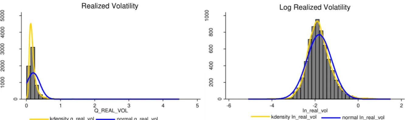
13 Figure 1 shows that realized volatility is negatively skewed and leptokurtic compared to a normal distribution. Figure 2 indicates that log realized volatility roughly fits a log-normal distribution. For this reason I use log realized volatility in my analysis.
Figure 1: Density plot – Realized Volatility Figure 2: Density plot – Log Realized Volatility
IV. Hypothesis Development and Research Design
I divide my empirical analysis into four stages. First I check if the fundamental variables above described are related with future volatility. Second, based on the literature discussed in Section II.2 I find the traditional volatility model that best fits my data. Third, I test the significance of each financial variable incremental to the model estimated. Finally I design an investment strategy to try to ‘arbitrage’ on volatility. In this chapter, I describe the methodology and assumptions followed in each stage of my analysis. According to what was already described, I can formulate my first hypothesis as follows: Hypothesis 1: Financial information of a firm is related with the future volatility of
that firm’s stock returns. Volatility increases with leverage, cash flow volatility, personnel
expenses, book-to-market ratio and earnings opacity and decreases with size and return
on assets.
I test this hypothesis by estimating equation (5) systematically for each of the eight variables that are being considered and testing the significance of β1
σ𝑖,𝑅𝑉𝑡+𝜏 = β0 + β1V_FSV𝑖,𝑗𝑡 + β2 Year + ε𝑖,𝑡 (5)
0
1000
2000
3000
4000
5000
0 1 2 3 4 5
Q_REAL_VOL kdensity q_real_vol normal q_real_vol
Realized Volatility
0
200
400
600
800
1000
-6 -4 -2 0 2
ln_real_vol
kdensity ln_real_vol normal ln_real_vol
14 V_FSV𝑗
𝑖,𝑡, (j=1, … , 8), is an indicator variable that equals one if the level of the
accounting based variable j for firm i is above its industry median and equals zero otherwise. For instance, V_SIZE is one if firm i in quarter t was larger than the median of its respective industry according to the computations made in section III. The estimation of equation (5) uses fixed effects and slightly differs from the estimation of equation (3) presented in section II. While Sridharan (2015) follows a two-way industry and quarter clustered standard errors approach I follow Petersen (2009), who argues that, in panels with more firms than years, the best approach is to absorb time effect by the inclusion of a dummy variable for years and then cluster by firm. I found no evidence of being necessary to control in two time dimensions, both by year and by quarter. From Figures 3 and 4 one realizes that the dependent variable presents some heterogeneity by year, but almost none by quarter. Moreover, to include a control for industry would be redundant, since the construction of the dependent variables already considers the relationship between a firm and its respective industry. Nevertheless, non-tabulated results show that there are no qualitative differences if the estimation is made clustering in two dimensions by industry and quarter, industry and country, or country and quarter.
Figure 3: Year Effects: Heterogeneity across years Figure 4: Quarter Effects: Heterogeneity across quarters
To find the volatility model that best fits my data I first have to convert the panel dataset I am using into a time series. Since Cermeno and Grier (2001) there have been
-6
-4
-2
0
2
2004 2005 2006 2007 2008 2009 2010 2011 2012 2013 2014 2015 Year
ln_real_vol ln_vol_mean
-6
-4
-2
0
2
1st 2nd 3rd 4th
Quarter
15 some experiences trying to adapt ARCH models to a panel data context. However, I chose not to follow this approach for two reasons. First, Stata does not have an installed routine for this adaptation and an accurate replication of the process introduced by Cermeno and Grier (2001) requires substantial Stata programming skills. Second, this extension relies on the assumption that the disturbances in the model are cross-sectionally independent. This would not probably hold in my sample, since many firms belong to the same industries and countries. An alternative way to address this problem would then be to use the multivariate GARCH model, introduced by Bollerslev, Engle & Wooldridge (1988) in which the conditional covariance matrix H at time t (for GARCH(1,1) specification) is given as
vech(Ht) = C + Avech(ε𝑡−1𝜀𝑡−1′ ) + Bvech(Ht-1)
However, being heavily parameterized, multivariate GARCH is tractable only for a small number of series. For example, a sample composed by only three firms requires an estimation of 78 coefficients. Even with the simplification assumptions of Bollerslev, Engle & Wooldridge, who assume the matrices A and B are diagonal, the number of coefficients to be estimated is still very large (18). A sample as the one I am using would require a not reasonable number of coefficients to be estimated. Moreover, the main applications of multivariate GARCH are conditional CAPM, futures hedging and volatility spillovers modeling, which are not the main focus of my research. Therefore, I aggregate the firms of my sample into an index, weighted by the market capitalization of each firm in the previous day of the earnings announcement.
To choose the mean equation for the volatility models of the index, I considered the Autoregressive Moving Average model (ARMA)
16 and estimated it for different values of m and n with and without the constant term c. I then compare the Bayesian Information Criterion of each estimation to decide which ARMA(m,n) to use on the volatility models.2
Some of the most complex ARCH family models, such as CGARCH, GARCH-M, or AGARCH, require a considerable amount of data to be estimated. Because my sample is composed by quarterly observations and the time series is relatively small, only some of the most basic specifications were considered.
For (6) I considered the specifications ARCH(q) where σ2𝑡 = ω + 𝛼𝑖 ∑𝑞𝑖=1 u𝑡−𝑖2 , GARCH(q,p), where σ2𝑡 = ω + ∑𝑞𝑖=1 𝛼 𝑖 u𝑡−𝑖2 + β𝑗 ∑𝑞𝑗=1 σ𝑡−𝑗2 , EGARCH(1) where
ln(σ2
𝑡) = ω + 𝛼[ |𝑢𝑡−1 | √σ2 𝑡−1
− √2𝜋] + ϒ 𝑢𝑡−12
√σ𝑡−12 + β ln (σ 2
𝑡−1) with ϒ being a component for leverage
effects and PGARCH(1,1,1) where σ𝑡 = ω + ∑𝑞𝑖=1 𝛼(|𝑢𝑡−1 | + ϒ𝑢𝑡−1 ) + ∑𝑞𝑖=1 βσ𝑡−𝑗 . I then compared, the Bayesian Information Criterion of each estimation to decide on the volatility model most suitable for my data. After that, I tested a second hypothesis, formulated as follows:
Hypothesis 2: For stocks without options, the estimation of realized volatility using
an ARCH family model can be improved with the inclusion of variables based on
accounting information.
I did so by adding the financial variables that showed significance when testing Hypothesis 1 and analyzing the new model. All the referred estimations were done
considering only the first 30 observations of the index and using robust estimators. The remaining were left for out-of-sample tests.
17 V. Results
According to the methodology described above, this section presents and analyzes the main results of my research. All estimations were obtained using Stata13.
V.1 Hypothesis 1
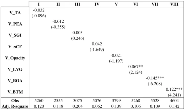
The estimation results of equation 5 that tests Hypothesis 1 is summarized in table 3.
Table 3: Regression of Log Realized Volatility on accounting-based fundamental variables – Summary of results. t-statistics in parenthesis below coefficients. ***, ** and * indicate statistical significance at 1, 5 and 10 percent, respectively.
From the table, Size, Personal Expenses to Assets, Sales Growth, Cash Flow Volatility and Earnings Opacity show no significant statistical correlation with the dependent variable. However, Leverage and Book-to-Market ratio are positively related to volatility and Return on Assets is negatively related to it. These three variables present coefficients significantly different from zero – Leverage at 5% significance level and the others at 1% significance level – and relate to volatility in the way predicted in Section II.1. The interpretation of the coefficients must consider the fact that the dependent variable is a logarithm. Therefore, the coefficient 0.067 on Leverage, for instance, indicates that firms with a level of leverage above their industry’s median, have on average 6.7% higher
I II III IV V VI VII VIII
-0.032 (-0.896) -0.012 (-0.355) 0.003 (0.246) 0.042 (-1.649) -0.021 (-1.197) 0.067** (2.124) -0.145*** (-6.208) 0.122*** (4.241)
Obs 5260 2555 3075 5076 3799 5260 5528 4604
18 returns volatility than firms below the industry median. Comparing these results with those of Sridharan (2015), a substantial difference is easily noted. Despite still positive to support that fundamental variables are related with realized volatility (Hypothesis 1), my results are not so good, considering either the number of relevant variables or the adjusted R-Square of the estimations. It is a fact that a much lower number of observations were used. However, that number should be enough to produce efficient estimates. The methodology used was virtually the same and the variables were constructed in a similar way. I am, therefore, lead to conclude that differences in the data are responsible for differences in results. It is important to consider that I used a more recent dataset than Sridharan, with firms of a different geographic location and with different specific features.
V.2 Mean Equation of the Volatility Models
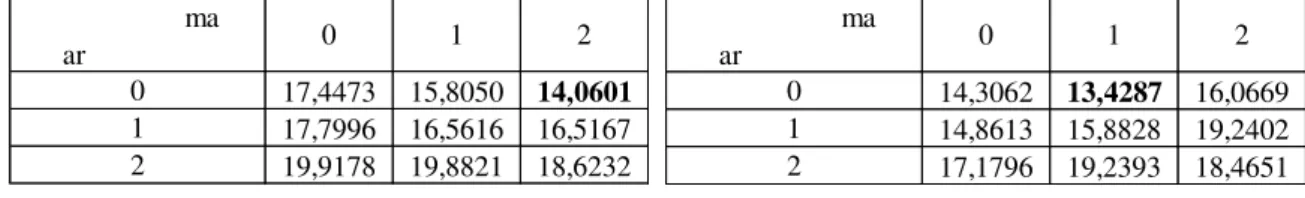
The Bayesian Information Criterion resulting from the estimation of ARMA(q,p) models with q={0,1,2} and p={0,1,2} is summarized in tables 4 and 5.
Table 4: Bayesian Information Criterion on ARMA(q,p) estimations. With constant term.
Table 5: Bayesian Information Criterion on ARMA(q,p) estimations. Without constant term.
From the tables above it is possible to observe that removing the constant term usually improves the results of the estimation. Moreover, the best fitted model is a ARMA(0,1) with no constant. Performing a Portmanteau test for white noise on the chosen specification and using 12 lags (value chosen by default), a Q statistic of 6.6983 was obtained. Comparing it to a χ2 distribution with 12 degrees of freedom, one does not reject the null hypothesis of no autocorrelation in the residuals, indicating that the residuals apparently behave as white noise, as is desired.
17,4473 15,8050 14,0601 17,7996 16,5616 16,5167 19,9178 19,8821 18,6232
2
1 2 0 ar
ma 0 1
14,3062 13,4287 16,0669 14,8613 15,8828 19,2402 17,1796 19,2393 18,4651 ar
ma
1 2
0 1 2
19 V.3 Volatility Models
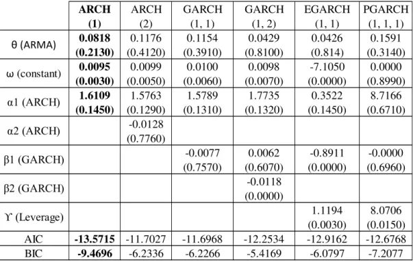
Using the ARMA(0,1) specification for the mean equation, different volatility models were estimated. The results are summarized in Table 6.
Table 6: ARCH family volatility models. P-values in parenthesis below coefficients.
Analyzing the values of Akaike’s Information Criteria (AIC) or the values of Bayesian Information Criterion (BIC), the conclusion is that ARCH(1) is the model that best fits the data used. The fact that the most basic specification is the one that presents a lower AIC and BIC can probably be explained by the small size of the time series, since in the absence of long high frequency data, the estimation procedure might favor the model with less parameters. Despite that, performing an ARCH-LM test, with 1 lag, on 𝜎̂𝜀̂22 results in a Q statistic of 0.7700. Comparing it to a χ2 distribution with 1 degree of freedom, one does not reject the null hypothesis of no arch effect, indicating that the chosen model is sufficient to capture potential arch effects in the data.
ARCH ARCH GARCH GARCH EGARCH PGARCH
(1) (2) (1, 1) (1, 2) (1, 1) (1, 1, 1)
0.0818 0.1176 0.1154 0.0429 0.0426 0.1591
(0.2130) (0.4120) (0.3910) (0.8100) (0.814) (0.3140)
0.0095 0.0099 0.0100 0.0098 -7.1050 0.0000
(0.0030) (0.0050) (0.0060) (0.0070) (0.0000) (0.8990)
1.6109 1.5763 1.5789 1.7735 0.3522 8.7166
(0.1450) (0.1290) (0.1310) (0.1320) (0.1450) (0.6710)
-0.0128 (0.7760)
-0.0077 0.0062 -0.8911 -0.0000 (0.7570) (0.6070) (0.0000) (0.6960)
-0.0118 (0.0000)
1.1194 8.0706 (0.0030) (0.0150)
AIC -13.5715 -11.7027 -11.6968 -12.2534 -12.9162 -12.6768
BIC -9.4696 -6.2336 -6.2266 -5.4169 -6.0797 -7.2077
β2 (GARCH)
ϒ (Leverage) θ (ARMA)
ω (constant)
α1 (ARCH)
α2 (ARCH)
20 V.4 Hypothesis 2
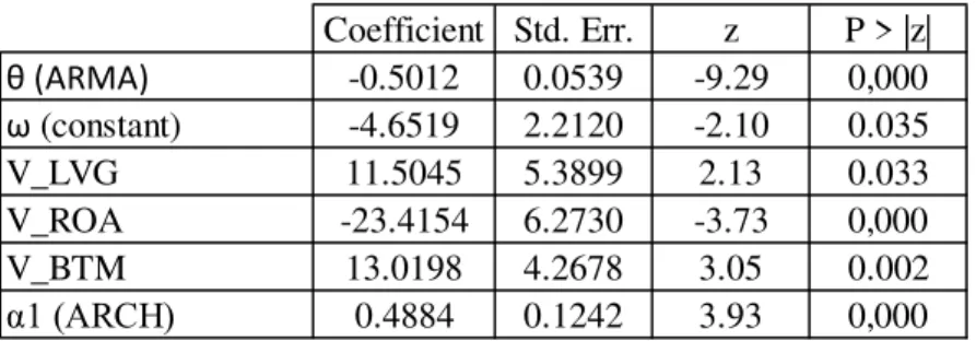
To test the second hypothesis I added to the model the variables that showed significance in V.1: Leverage, Return on Assets and Equity Book-to-Market Ratio. The estimation results are summarized in Table 8.
Table 8: ARMA(0,1) – ARCH(1) with financial variables.
The results are substantially positive and support Hypothesis 2. All coefficients are significant, the constant term and leverage at 5% and the remaining at 1% significance level. Most important, the financial variables influence volatility as predicted – Leverage and Book to Market have a positive sign and Return on Assets has a negative sign. Moreover, the inclusion of the financial variables reduced AIC from -13.5715 to -15.5264 and BIC from -9.4696 to -9.9779 and a Likelihood Ratio test on the variables added to the model shows a Q-statistic of 7.95 which, compared to a χ2 distribution with 3 degrees of freedom, indicates overall significance of the financial variables.
V.5 Systematic Trading Strategy
Having better forecasts than the market can be very profitable. The positive results of Table 8 suggest the possibility for a volatility arbitrage opportunity that I will try to explore. To design a trading strategy I assume that the market uses the ARMA(0,1) ARCH(1) model to estimate volatility. This seems reasonable to assume, since it is the model that better fits historical quarterly market returns. Instead, I use the same model, but improved by the inclusion of financial variables. I also assume that the market uses returns volatility as a relevant measure of risk and that market estimations are included in
Coefficient Std. Err. z P > |z|
θ (ARMA) -0.5012 0.0539 -9.29 0,000
ω (constant) -4.6519 2.2120 -2.10 0.035
V_LVG 11.5045 5.3899 2.13 0.033
V_ROA -23.4154 6.2730 -3.73 0,000
V_BTM 13.0198 4.2678 3.05 0.002
21 stock prices. This should be also reasonable to assume, according to Markowitz (1952) and Fama (1970). Therefore, if my model indicates a lower volatility than what it is estimated by the market I will be long on the stock. I do so, because in the current price of the stock, would be implied a higher risk profile than the one the stock actually has. Therefore, investors ‘demand’ a higher return than what would be fair. I will be out of the
market in the opposite condition, to avoid incurring in excessive risk.
Using the observations included in the estimation of the models, the strategy would earn substantial returns, presenting an annual average of 9.12% net of the market for a Sharpe Ratio of 0.2. This result confirms that the model with financial variables is better, in-sample, than the simple ARMA(0,1) ARCH(1) and shows that the assumptions of my strategy hold in this market. However, an out-of-sample strategy would allow a more accurate analysis of the real forecasting power of my model. This way, I apply the same strategy only to the 16 last quarterly observations (4 years of data). The results are not so good, but still positive – an annual average of 0.92% net of the market and a Sharpe Ratio of 0.06. The strategy is better than a passive investment on the index, due to the fact that it keeps us out of the market in periods of high volatility, increasing the expected return and decreasing the standard deviation of the investment. To note that the observations to which the strategy applies were not used in the estimation process and that the variables were constructed in a way to avoid using information not available to market participants. Therefore, these results are free of any forward looking bias and reflect a true increment to the volatility model given by the financial variables.
22 VI. Conclusions
My research enhances a recent link between financial accounting information and volatility modeling. I show that Leverage and Equity Book-to-Market Ratio (positively) and Return on Assets (negatively) are related with realized volatility and that the inclusion of those variables in an ARCH(1) model provides an increment to its explanative power. I also construct a successful investment strategy, which explores the superior forecast performance of the model with financial variables.
I show that using financial information has the advantage of improving the estimation results of a volatility model. However, a drawback of this approach should also be considered. By using information collected from financial statement figures, one is significantly reducing the number of observations. Instead of daily prices, for instance, we are forced to use quarterly observations and this can impact the choice of the correct model specification. Nevertheless, estimating volatility this way can still be useful, namely for medium/long term investments.
23 The results contribute to the volatility modeling literature in the sense that they were able to establish a relationship between a traditional ARCH volatility model and a set of financial variables. Considering that there are still many firms that do not have stock options trading on an exchange, there are several applications to a model of this nature, such as risk management, investment decisions or pricing spreads or financial instruments such as defaultable bonds.
VII. References
Alexakis, Christos; Patra, Theophano and Poshakwale, Sunil. 2010. "Predictability of Stock Returns using Financial Statement Information: Evidence on Semi-strong Efficiency of Emerging Greek Stock Market." Applied Financial Economics, 20(16): 1321-1326.
Allayannis, George and Weston, James. 2005. "Earnings Volatility, Cash Flow volatility, and firm value.” Working Paper.
Beaver, William. 1966. “Financial Ratios as Predictors of Failure.” Journal of Accounting Research, 4: 71-111.
Beaver, William; McNichols, Maureen and Rhie, Jung-Wu. 2005. “Have Financial Statements Become Less Informative? Evidence from the Ability of Financial Ratios to Predict Bankrupcy.” Review of Accounting Studies, 10: 93-122.
Bollerslev, Tim; Engle, Robert and Wooldridge, Jeffrey. 1988. “A Capital Asset Pricing Model with Time Varying Conditional Covariances.” Journal of Political Economy, 96: 116-131.
24 Caneghem, Tom; Campenhout, Geert and Uytbergen, Steve. 2002. "Financial Statement Information and the Prediction of Stock Returns in a Small Capital Market: The Case of Belgium." Brussels Economic Review, 45(3): pp. 65-90.
Cermeno, Rodolfo and Grier, Kevin. 2001. “Modeling GARCH Processes in Panel Data: Theory, Simulations and Examples.” CIDE, Working Paper.
Chan, Louis; Lakonishok, Josef and Sougiannis, Theodore. 2001. "The Stock Market Valuation of Research and Development Expenditures." The Journal of Finance, 56(6): 2431-2457.
Chen, Nai-fu and Zhang, Feng. 1998. "Risk and Return of Value Stocks." The Journal of Business, 71(4): 501-535.
Christensen, Bent and Strunk, Charlotte. 2002. "New Evidence on the Implies-Realized Volatility Relation." The European Journal of Finance, 8(2): 187-205.
Claessen, Holger and Mittnik, Stefan. 2002. "Forecasting Stock Market Volatility and the Informational Efficiency of the DAX-index Options Market." Center of Financial Studies, Working Paper No. 2002/04.
Eklund, Trond; Larsen, Kai and Bernhardsen, Eivind. 2001. "Model for analysing credit risk in the enterprise sector." Norges Bank Economic Bulletin, 3(01): 99-106. Engle, Robert. 1982. “Autoregressive Conditional Heteroscedasticity with Estimates of the Variance of United Kingdom Inflation.” Econometrica, 50(4): 987-1087.
Fama, Eugene. 1970. "Efficient capital markets: A review of theory and empirical work." Journal of Finance, 25(2): 427-465.
Fama, Eugene and French, Kenneth. 1992. "The Cross-Section of Expected Stock Returns." The Journal of Finance, 47(2): 427-467.
25 Goodman, T.; M. Neamtiu and F. Zhang. 2013. “Fundamental Analysis and Option Returns”, Working Paper.
Goslim, Jonathan; Chai, Daniel and Gunasekarage, Abeyratna. 2012. “The Usefulness of Financial Statement Information in Predicting Stock Returns: New Zealand Evidence.” Business and Finance Journal, 6(2): 51-70.
Gow, Ian; Ormazabal, Gaizka and Taylor, Daniel. 2009. “Correcting for Cross-Sectional and Time-Series Dependence in Accounting Research.” The Accounting Review, 85(2): 483-512.
Grullon, Gustavo; Lyandres, Evgeny and Zhdanov, Alexei. 2012. “Real Options, Volatility, and Stock Returns.” Journal of Finance, 67: 1499-1536.
Hui, Cho; Lo, Chi-Fai and Huang, M. 2007. "Predictions of Default Probabilities by Models with Dynamic Leverage Ratios." SSRN Electronic Journal, DOI: 10.2139/ssrn.1113726.
Hutton, Amy; Marcus, Alan and Tehranian, Hassan. 2009. “Opaque Financial Reports, R-Square, and Crash Risk.” Journal of Financial Economics, 94: 67-86.
İlker, Gökbulutand and Mehmet, Pekkaya. 2014. “Estimating and Forecasting
Volatility of Financial Markets Using Asymmetric GARCH Models.” International Journal of Economics and Finance, 6(4): 23-35.
Kaplan, Robert and Gabriel Urwitz. 1979. "Statistical Models of Bond Ratings: A Methodological Inquiry." Journal of Business, 52(2): 231–261.
Malkiel, Burton. 2003. “The Efficient Market Hypothesis and Its Critics.” Journal of Economic Perspectives, 17(1): 59-82.
26 Maricica, Moscalu and Georgeta, Vintila. 2012. "Business Failure Risk Analysis Using Financial Ratios." Procedia – Social and Behavioral Sciences, 62: 728-732.
Markowitz, Harry. 1952. "Portfolio Selection." The Journal of Finance, 7(1): 77-91. Minton, Bernadette and Schrand, Catherine. 1999. “The Impact of Cash Flow Volatility on Discretionary Investment and the Costs of Debt and Equity Financing.” Journal of Finance Economics, 54(3): 423-460.
Palepu, Krishna. 1986. "Predicting Takeover Targets: A Methodological and Empirical Analysis." Journal of Accounting and Economics, 11(8): 3-35.
Petersen, Mitchell. 2009. "Estimating Standard Errors in Finance Panel Data Sets: Comparing Approaches." Review of Financial Studies, 22(1): 435-480.
Poon, Ser-Huang and Granger, Clive. 2003. “Forecasting Volatility in Financial Markets: A Review.” Journal of Economic Literature, 41(2): 478-539.
Roberts, SW. 1959. “Control Chart Tests Based on Geometric Moving Averages.” Technometrics, 1(3): 239-250.
Sinclair, Euan. 2013. “Volatility Forecasting Using Fundamental Information” in Volatility Trading, 2nd Edition. New Jersey: Wiley.
Sridharan, Suhas. 2015. “Volatility Forecasting Using Financial Statement Information.” The Accounting Review, 90(5): 2079-2106.