DEFINING MANAGEMENT ZONES BASED ON SOIL ATTRIBUTES AND
SOYBEAN PRODUCTIVITY
1FABRICIO TOMAZ RAMOS2*, RAUL TERUEL SANTOS3, JOSÉ HOLANDA CAMPELO JÚNIOR2, JOÃO CARLOS
DE SOUZA MAIA2
ABSTRACT – Demarcating soil management zones can be useful, for instance, delimiting homogeneous areas and selecting attributes that are generally correlated with plant productivity, but doing so involves several different steps. The objective of this study was to identify the chemical and physical attributes of soil and soybean plants that explain crop productivity, in addition to suggesting and testing a methodological procedure for defining soil management zones. The procedure consisted of six steps: sample collection, data filtering, variable selection, interpolation, grouping, and evaluation of management zones. The samples were collected in an experimental area of 12.5 ha cultivated with soybean during the 2013/14 crop in Dystrophic Red Latosol, in Mato Grosso, Brazil. A total of 117 pairs of plant and soil samples were collected. Student’s t-test was used (α = 0.02) to verify that the number of samples was adequate for correlation analysis. Results showed that only the P and Mn content in the grains explained (based on R2 values) the variation in soybean grain productivity the area. Based on the interpolation of these contents by ordinary kriging, the fuzzy C-means algorithm was used to separate them into groups by similarity. Division into two groups was the best option, which could be differentiated by Mann–Whitney test (P < 0.05), resulting in a map with 10 management zones.
Keywords: Glycine max L.. Direct seeding. Precision agriculture.
DEFINIÇÃO DE ZONAS DE MANEJOS A PARTIR DE ATRIBUTOS DO SOLO E PRODUTIVIDADE DE SOJA
RESUMO - Zonas de manejo do solo são usadas, por exemplo, para delimitar áreas homogêneas, selecionando atributos que no geral correlacionam com a produtividade das plantas, mas, defini-las requer diferentes etapas. Objetivou-se neste trabalho identificar atributos químicos e físicos do solo e de plantas de soja que explicaram a produtividade de grãos da cultura e, também, sugerir e testar um procedimento metodológico para definir zonas de manejo do solo. O procedimento consistiu de seis etapas: coleta de amostras, filtragem dos dados, seleção das variáveis, interpolação, agrupamento e avaliação das zonas de manejo. As amostras foram coletadas em uma área experimental de 12,5 ha, cultivada com soja na safra 2013/14, em um Latossolo Vermelho Distrófico, em Mato Grosso, onde foram coletados 117 pares de amostras de plantas e de solo. Utilizando-se o teste de Student (α = 0,02), verificou-se que o número de amostras foi adequado para a análise de correlação. Entretanto, apenas os teores de P e Mn dos grãos explicaram (R2) a variação da produtividade de grãos de soja
na área. Com base na interpolação destes teores por krigagem ordinária utilizou-se o algoritmo fuzzy C-means para separá-los em grupos por similaridade, em que a divisão em 2 grupos foi a melhor opção, que diferiram pelo teste de Mann-Whitney (P < 0,05), resultando em um mapa com 10 zonas de manejo.
Palavras-chave: Glycine max L.. Plantio direto. Agricultura de precisão.
_____________________ *Corresponding author
1Received for publication in 04/30/2016; accepted in 11/28/2016.
Rev. Caatinga
INTRODUCTION
Farmers in the state of Mato Grosso, Brazil are increasingly adopting precision agriculture techniques, such as variable rate fertilization using agricultural equipment with a global positioning system. However, care must be taken during automatic defining of management zones based on precision agriculture software, because according to Yamamoto and Landim (2013), instead of homogenizing soil fertility, it might increase its spatial variability.
Variable rate fertilization is useful to avoid underestimation or overestimation of limestone and fertilizer dosages. However, some issues might need attention, for example, (i) poorly performed field sampling could lead to errors in the interpretation of analysis results; therefore, no matter how sophisticated the laboratory analyses are, they would be unable to correct the shortcomings of inadequate data collection or sampling methods that do not effectively isolate the sources of variation (YAMAMOTO; LANDIM, 2013; FU et al., 2016); (ii) during geostatistical analysis, the ideal quantity of samples needed for routine analysis vs. the number judged by the farmer as economically viable for sending to the laboratory might differ, and therefore, the veracity of the georeferenced maps could be compromised (TEY; BRINDAL, 2012; YAMAMOTO; LANDIM, 2013); and (iii) even if the sampling is representative and judicious, there could be other problems related to the initial diagnosis of errors and methodical statistical processing of raw data (HAIR JR. et al., 2009; TAYLOR; BATES, 2013; FU et al., 2016). Thus, factors that can affect the quality of maps processed without minimum criteria with respect to statistical analysis and geostatistics should be kept in mind.
Another issue concerns the costs involved in sampling schemes and soil and plant analyses, which were questioned by farmers in Mato Grosso with respect to their practical and economic viability. Defining management zones requires various steps, from data collection to map evaluation, based on which the cultivation area is divided into subareas that have homogeneity with respect to the evaluated attributes (RODRIGUES; CORÁ; FERNANDES, 2012; ALVES et al., 2013; FARID et al., 2013; DALCHIAVON et al., 2013; BAZZI et al., 2015; SANTOS et al., 2015; SANTOS; SARAIVA, 2015). This allows the application of inputs at appropriate rates for improving the productivity of a crop (BREDEMEIER et al., 2013; BAGHERI et al., 2013; COSTA et al., 2014). However, it is common to see variations in sampling methods, laboratory analyses, statistics, and geostatistics, irrespective of their correlation with plant productivity (ALVES et al.
2013; BREDEMEIER et al., 2013; URRETAVIZCAYA et al., 2014).
Because of variations in the stages of analysis for defining management zones and considering the reference processes proposed by Santos and Saraiva (2015), it can be assumed that formalization of a general support model is possible, that is, a flowchart to assist in the definition of soil management zones. This flowchart is initially intended to represent the essential basic steps for defining management zones, considering only the variables controllable by the farmer, which relate to the productivity of the plants. The objective of this work was to identify chemical and physical attributes of soil and soybean plants that explain the grain productivity of the crop, and to suggest and test a methodological support procedure to define soil management zones.
MATERIAL AND METHODS
Location descriptionThis study was carried out on a farm in the
city of Diamantino-MT, Brazil (latitude 14° 07′ 40′′ S, longitude 56° 58′ 39′′ W), at an
altitude of 539 m. The climate of the region is Aw according the classification of Köppen. The average annual precipitation is 1816.9 mm. The average annual temperature is 25.5 °C. The soil of the experimental unit was classified as typical Dystrophic Red Latosol, moderate A, very clayey texture, semi-deciduous tropical forest and flat relief (SANTOS et al., 2013).
In 1987, the native vegetation was cleared and rice was sown in the 1987/88 crop. From 1989/90 until the 1999/2000 crop, soybean and corn were grown in succession, with fertilizers applied in the seeding row. From 2000/01 until the 2003/04 crop, cotton was grown. From 2004/05 to the 2013/14 crop, soybean and corn were grown in succession, without ploughing the soil, with limestone and fertilizers applied by broadcasting. For the present study, in the 2013/14 crop, the soybean crop was evaluated (Glycine max L.). On an experimental unit of approximately 12.5 ha of a 55-ha-plot, cultivar MONSOY 7639 RR was cultivated with a spacing of
0.45 m between rows and an average of 15 plants m-1. The sowing was done on October 23,
2013 and harvest on February 5, 2014.
Sample collection
Soil and plant sampling was of the irregular mesh type, because of deviations of the contour lines of the culture, totaling 117 collection points. According to Yamamoto and Landin (2013), a minimum of 100 observations is recommended. The collection areas were georeferenced with maximum horizontal and vertical error of 0.05 m using a global positioning apparatus (brand Topcon Hiper®, Pro model).
The choice of attributes for the analyzed soil and plants, which are discussed below, was based on factors related to plant productivity (RODRIGUES; CORÁ; FERNANDES, 2012; ALVES et al., 2013; COSTA et al., 2014; BAZZI et al., 2015). Disturbed and undisturbed soil samples were collected, along with samples of plants during the phenological cycle of the crop. At R7.2 stage of the crop, taking into account the area explored by soybean roots, disturbed soil samples were collected from the 0 to 0.20 m layer, using a Dutch auger with a 0.20 m bucket, to determine the following attributes: sand, silt, and clay contents, using the pipette method (DONAGEMA et al., 2011), soil organic matter content, using the method of oxidation with potassium dichromate and colorimetric determination, pH in 0.01 M CaCl2 in 1:2.5 proportion (soil:CaCl2) exchangeable P and K, extracted with solution of 0.05 M HCl and 0.025 M
extracted with calcium acetate solution at pH 7 (SILVA, 2009).
Undisturbed soil samples were collected using a kopeck sampler to insert steel cylinders (50 mm in diameter and 50 mm in height) into the intermediate portion of 0 to 0.10 and 0.10 to 0.20 m layers to obtain average values for 0 to 0.20 m layer. A flat auger was used to level and control the sampling depth. The microporosity was determined in the laboratory with the aid of a tension table at 10 kPa, in addition to soil density, total porosity of the soil using particle density of each sampling point, and soil macroporosity using the difference between total porosity and microporosity (DONAGEMA et al., 2011).
Finally, soybean grain productivity (kg ha-1) at the R8 stage was estimated by harvesting 4 m of plants at each sampling point and correcting the grain moisture values to 14%. In the grain samples, the N content were determined by acid digestion, distillation, and titration (Kjeldahl method), in addition to P, K, Ca, Mg, S, Zn, Cu, Fe, Mn, and B concentrations, through simultaneous determination of multi-elements by atomic emission spectrometry with plasma induction (EEA-ICP) (SILVA, 2009).
Data Filtering
Rev. Caatinga
the data, Shapiro–Wilk test was used (α = 0.05) before and after the removal of possible outliers, following Hair Jr. et al. (2009).
Variable selection
The statistical assumptions inherent to the analyses of statistical correlation and linear regression (adequacy of sample size, linearity, homoscedasticity, and residual normality) were verified, following Hair Jr. et al. (2009).
The adequacy of the sample size was calculated according to the protocol of Hair Jr. et al. (2009), using the Student’s t distribution table at 2% error probability. Next, the independent variables were verified to determine the ones that explain the dependent variable, grain productivity (kg ha-1). For this, best subset regression analysis was done in Sigma Plot version 12.5, which avoids the occurrence of collinearity. The criteria used to select the best multiple linear regression model, following Hair Jr. et al. (2009), were variance inflation factor
(VIFi), adjusted coefficient of determination (R2 Aj.), and beta coefficient (β).
The accuracy of the multiple linear regression analysis, following Hair Jr. et al. (2009), was evaluated by the significance level of the fit using F-test (α = 0.05), regression coefficient (R²), and standard error of the estimate. The homoscedasticity
was evaluated by Spearman rank correlation (P > 0.05). The residual normality was evaluated
using Shapiro–Wilk test (P > 0.05) in Sigma Plot version 12.5.
Interpolation
The modeled semivariograms were verified as isotropic using the software Gamma Design version 10.0, with the data interpolated, following Yamamoto and Landin (2013), through ordinary kriging in 2 m × 2 m blocks. Cross-validation was done using linear regression analysis (P < 0.05) to validate the interpolation. After the cross validation was accepted, the interpolations were done using a pixel size of 1 m × 1 m for the X and Y coordinates and with the same contour polygon. According to Alves et al. (2013), this standardization ensures that all generated maps have the same number of pixels, allowing them to overlap.
Data grouping
The fuzzy C-means algorithm was used to combine the interpolated values, and then they were separated into groups by similarity based on Euclidean distance (FU; WANG; JIANG, 2010; RODRIGUES JUNIOR et al., 2011; DAVATGAR;
NEISHABOURI; SEPASKHAH, 2012). The values were standardized to the interval [0, 1], so that all the sampled values had the same scale of magnitude, defining in 100 the maximum number of interactions and in 1.3 the degree of ‘fuzzification’. The software R (The R Project for Statistical Computing) and the e1071 package (MEYER et al., 2015) were used for this purpose. Maps were generated with group numbers 2 through 6.
To determine the most appropriate number of groups, the Fuzzy Performance Index (FPI) and Normalized classification entropy (NCE) were used, which should converge to minimum values corresponding to the same class (FRIDGEN et al., 2004). The indices available in the fclustindex function of the e1071 package were also used: fuzzy hypervolume (Fhv), xie beni (Xb), partition entropy (Pe), where the lowest value indicates the best division or most similarity among the groups, and the average partition density (Apd) and partition density (Pd) indices, where the best division corresponds to the highest value (MEYER et al., 2015). Additionally, the cluster validation index (CVI) was used, where the smallest value indicates the best division (SCHENATTO et al., 2016).
Evaluation of management zones
To compare the values of the management zones, Hair Jr. et al. 2009 suggested that in case of observed unpaired values with a normal distribution, Student’s t-test should be used to compare the average values. Otherwise, in the absence of normality, the Mann–Whitney nonparametric test should be used to compare the average values, or the Kruskal–Wallis test, which is an extension of the Wilcoxon–Whitney test, for comparing three or more groups of unpaired values that do not meet the requirements for the analysis of variance (α = 0.05) (HAIR JR. et al., 2009). Therefore, the present study used the Mann–Whitney test.
RESULTS AND DISCUSSION
Table 1. Descriptive statistics for the analyzed attributes of soil.
Variables n
(1)
Min. Max. Average CV (%) P value
Shapiro–Wilk(2) N(3)
P (mg dm-3) 113 3.20 23.70 9.23 39.46 0.0514 3.009
Ca (cmolc dm-3) 113 1.00 4.00 2.73 11.67 0.6530 3.110
Mg (cmolc dm-3) 113 0.70 1.30 1.00 8.29 0.0830 1.218
k (cmolc dm-3) 113 0.07 0.28 0.12 38.13 0.1200 1.074
H (cmolc dm-3) 113 3.30 5.70 4.60 7.87 0.2890 4.143
Al (cmolc dm-3) 113 0.00 0.40 0.02 359.45 0.0561 1.770
SB (cmolc dm-3 113 2.70 5.40 3.85 12.27 0.3130 1.051
V (%) 113 34.40 59.20 45.43 10.25 0.3860 4.917
CTC (cmolc dm-3) 113 7.40 9.50 8.52 5.51 0.3840 1.050
pH (CaCl) 113 4.7 5.52 5.035 3.56 0.0510 1.293
Organic matter (g dm-3) 113 28.70 38.90 34.27 6.00 0.0582 1.959
Sand (g kg-1) 113
316 397 360.00 5.11 0.4360 77.173
Silt (g kg-1) 113 24 61 39 22.33 0.1100 17.402
Clay (g kg-1) 113 550 642 599 2.73 0.7080 60.869
Soil Density (Mg m-3) 113 1.22 1.39 1.30 3.18 0.3650 3.850
Total porosity (m3 m-3) 113 0.45 0.53 0.49 3.22 0.8380 5.620
Macroporosity (m3 m-3) 113 0.05 0.16 0.09 21.88 0.6700 9.750
Microporosity (m3 m-3) 113 0.36 0.42 0.40 3.21 0.5020 3.630
(1) Number of samples after removal of discrepant data (outliers); (2) Test of normality by Shapiro–Wilk test (P > 0.05); (3) Minimum number of necessary data points.
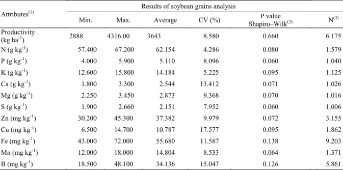
Table 2. Descriptive statistics for the analyzed attributes of soybean grains.
(1) Number of samples after removal of discrepant data (outliers); (2) Test of normality by Shapiro–Wilk test (P > 0.05); (3) Minimum number of necessary samples.
From the analyzed attributes of the soil (Table 1) and plants (Table 2) for the 113 samples, the grain productivity was found to be significantly correlated with the P and Mn content in the soybean grains. There was a positive correlation with the P
P < 0.01). Therefore, during multiple regression analysis with the P and Mn contents of the grains, it was verified that soybean grain productivity was explained in 19%, based on the coefficient of determination and with a standard error of estimate Attributes(1)
Results of soybean grains analysis
Min. Max. Average CV (%) P value
Shapiro–Wilk(2) N
(3)
Productivity
(kg ha-1) 2888 4316.00 3643 8.580 0.660 6.175
N (g kg-1) 57.400 67.200 62.154 4.286 0.080 1.579
P (g kg-1) 4.000 5.900 5.110 8.096 0.060 1.040
K (g kg-1) 12.600 15.800 14.184 5.225 0.095 1.125
Ca (g kg-1) 1.800 3.300 2.544 13.412 0.071 1.026
Mg (g kg-1) 2.250 3.450 2.873 9.368 0.070 1.016
S (g kg-1) 1.900 2.660 2.151 7.952 0.060 1.006
Zn (mg kg-1) 30.200 45.300 37.382 9.979 0.072 3.155
Cu (mg kg-1) 6.500 14.700 10.787 17.577 0.095 1.862
Fe (mg kg-1) 43.000 72.000 55.680 11.587 0.138 9.203
Mn (mg kg-1) 12.000 18.000 14.804 8.533 0.064 1.371
Rev. Caatinga
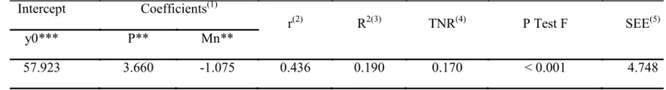
Table 3. Results of multiple linear regression analysis between phosphorus and manganese content in the soybean grains and soybean grain productivity.
Intercept Coefficients(1)
r(2) R2(3) TNR(4) P Test F SEE(5)
y0*** P** Mn**
57.923 3.660 -1.075 0.436 0.190 0.170 < 0.001 4.748
(1) P = phosphorus, g kg-1; Mn = manganese, mg kg-1; β = beta coefficient: P (β = 0.295), (β =
-0.264);
***(P < 0.0001), **(P < 0.01) by t-test; (2) r = Pearson correlation coefficient; (3) R2 = coefficient of determination;
(4) TNR = test of normality by Shapiro–Wilk test (P > 0.05); (5) SEE = standard error of the estimate, kg ha-1.
Therefore, P and Mn contents of the grains were the only attributes used to define the management zones in the present study. Dalchiavon et al. (2013), Costa et al. (2014), and Bazzi et al. (2015) also used only those attributes that showed significant correlation with crop productivity. As for the positive correlation between the grain P content and grain productivity, since the phosphate fertilization was applied by broadcasting from 2004/05 until 2013/14, according to Barbosa et al. (2015), a deficiency in P absorption by the plants could be occurring, since it concentrates on the soil surface. As a result, the availability of P has decreased in the soil to the extent that the correlation between its soil content and grain content is significant. This indicates that for producing more grains, it is necessary to correct this low availability of P. In the case of the observed negative correlation
for Mn, a high availability of this element in the soil could be an explanation, as described by Millaleo et al. (2010). The excess water in the soil that can transform Fe and Mn into soluble chemical forms that accumulate in the plant biomass, reaching toxic levels. When the plants absorb greater-than-adequate concentrations of Mn, it causes a reduction in grain productivity.
While analyzing the variability in the grain P content, a degree of spatial dependence of approximately 62% was observed, because of the nugget effect, and this variance was not explained by the geostatistical model. As for the variability in the grain Mn content, a high degree of spatial dependence of approximately 95% was observed and, therefore, there was little evidence for the nugget effect (Table 4).
Table 4. Results of the semivariogram adjustment of the P and Mn content in soybean grains.
Variable Parameters
(1)
R2 (2) N (3)
Model Co Co + C Co/ Co + C A
Pgrains Gaussian 0.07760 0.20520 0.622 145.4923 0.842 113
Mngrains Spherical 0.07600 1.67500 0.955 32.2000 0.786 113
(1) C
o = nugget effect, C = level, A = range; (2) R2 = coefficient of determination; (3) N = data pairs used.
It was observed that the distance (A), on which the points were spatially dependent, was higher for the grain P content, although with a degree of spatial dependence lower than the grain Mn content (C/Co+C = 0.955) (Table 4). According to Salviano, Vieira, and Sparovek (1998), this
suggests that the samples in the case of P content should have been taken at even shorter distances to reduce the nugget effect, in contrast to the Mn content. Next, cross-validation analysis of the observed data versus the data estimated by kriging was done (Table 5).
Table 5. Results of the cross-validation analysis using linear regression.
Variable Intercept Coefficient N (1) r R2 P
Test F SEE
P - Test
y0 a TNR(2)
Pgrains 2.595 ***
0.493*** 113 0.682 0.465 < 0.0001 0.232 0.0526
Mn grains 12.597*** 0.155** 113 0.374 0.140 0.0001 0.490 0.3677
(1) N = pairs of data used to adjust the model; (2) TNR = test of normality of Shapiro–Wilk (P > 0.05). Obs. *** (P < 0.0001), ** = significant (P < 0.01) by t-test.
Studies that contain cross validation information are rare, but cross validation is essential to evaluate the interpolation capacity of the model (ALVES; VECCHIA, 2011; COSTA et al. 2014; BOTTEGA et al., 2014). Therefore, from the Kriging cross-validation of the observed data for grain P content, an intermediate explanation of
variance was obtained (R2 ≈ 0.5), and for the grain
Mn content, a low explanation was obtained (R2 ≈ 0.14), both with a low estimation error.
significant (P < 0.05), the cross validations were accepted and the observed data were interpolated.
Subsequently, based on the interpolated data
for the P and Mn content in grains, the fuzzy C-means algorithm was used to group the data by
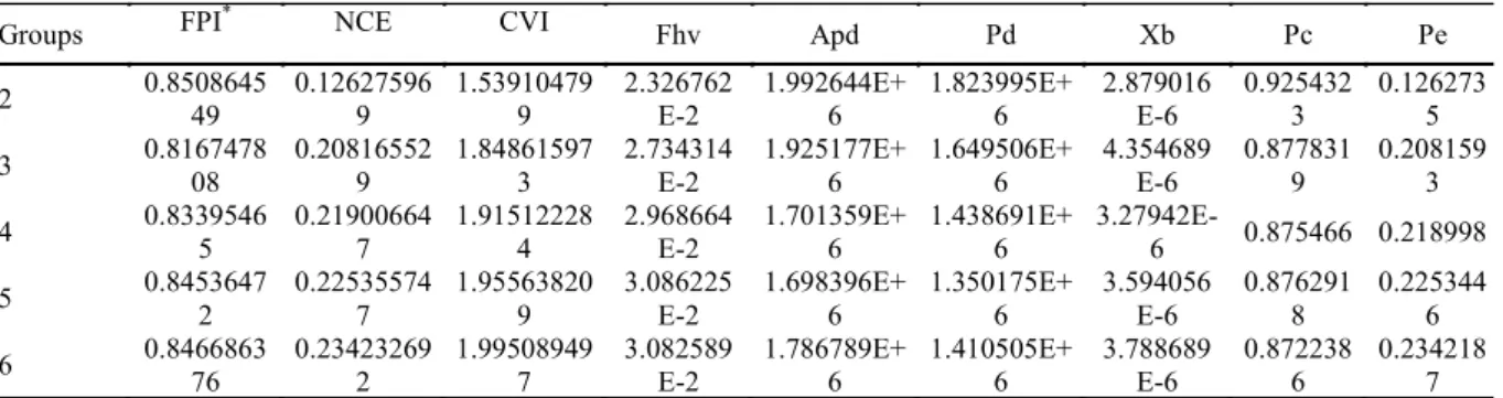
similarity. However, since the FPI and NCE indices did not converge to the same number of groups, we decided to independently analyze each of the indices
used, choosing the map indicated by most indices. This way, most of the indices described in the methods (NCE, Fhv, Apd, Pd, Xb, Pc, Pe, and VCI), which were used to define the appropriate number of groups, indicated that division into two groups was the best option; only the FPI indicated three groups as the best division (Table 6).
Table 6. Calculated indices for different groups of management zones.
Groups FPI
*
NCE CVI Fhv Apd Pd Xb Pc Pe
2 0.8508645
49 0.12627596 9 1.53910479 9 2.326762 E-2 1.992644E+ 6 1.823995E+ 6 2.879016 E-6 0.925432 3 0.126273 5
3 0.8167478
08 0.20816552 9 1.84861597 3 2.734314 E-2 1.925177E+ 6 1.649506E+ 6 4.354689 E-6 0.877831 9 0.208159 3
4 0.8339546
5 0.21900664 7 1.91512228 4 2.968664 E-2 1.701359E+ 6 1.438691E+ 6
3.27942E-6 0.875466 0.218998
5 0.8453647
2 0.22535574 7 1.95563820 9 3.086225 E-2 1.698396E+ 6 1.350175E+ 6 3.594056 E-6 0.876291 8 0.225344 6
6 0.8466863
76 0.23423269 2 1.99508949 7 3.082589 E-2 1.786789E+ 6 1.410505E+ 6 3.788689 E-6 0.872238 6 0.234218 7
*FPI – Fuzzy performance index; NCE – Normalized classification entropy; CVI – Cluster validation index; Fhv – Fuzzy hypervolume; Apd – Average partition density; Pd – Partition density; Xb – Xie beni index; Pe – Partition entropy.
As the number of groups increases, the management zones become more irregular, and if they present a small area, management might be unfeasible due to technical and economic limitations. Therefore, the final decision depends on the adequacy indices and results of successive tests of
Rev. Caatinga
According to Taylor, Mcbratney, and Whelan (2007), a management zone is a spatially continuous area, in which a particular treatment can be applied. Therefore, management zones are understood as the number of continuous subareas delimited within the experimental unit, which were ten in numbers in the present study. However, a given color indicates a class or group requiring the same treatment, within a range of values, which are the grouped contents of P
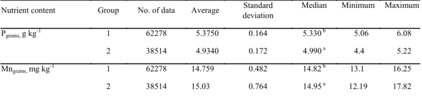
and Mn of the grains, that is, group 1 (green color) and group 2 (red color). The two groups that resulted in 10 management zones showed a significant difference in their median values, by Mann–Whitney test (P < 0.05) (Table 7). Thus, two groups or class intervals of distinct values were obtained, totaling ten management zones or homogeneous subareas in the study area.
Table 7. Comparison of the P and Mn content in soybean grains between the two data groups, which defined 10 management zones.
Nutrient content Group No. of data Average Standard
deviation
Median Minimum Maximum
Pgrains, g kg-1 1 62278 5.3750 0.164 5.330 b 5.06 6.08
2 38514 4.9340 0.172 4.990 a 4.4 5.22
Mngrains, mg kg -1
1 62278 14.759 0.482 14.82 b 13.1 16.25
2 38514 15.03 0.764 14.95 a 12.19 17.82
*Average values that change the letter in superscript differ by the Mann–Whitney test (P < 0.05).
Regarding the implications of the obtained results, there are some caveats. According to Table 3, grain productivity was affected by 19%, because of the spatial variability of P and Mn content in soybean grains. According to Table 7, comparing groups 1 and 2 indicated an average difference of 0.44 g kg-1
for P and of 0.271 g kg-1 for Mn. If an average 3500 kg of soybeans per hectare are harvested, 19%
of that is 665 kg. In other words, if a 60 kg sack of soybeans is sold at R$ 65.00, 665 kg equal a loss of 665/60 = 11.08 sacks or 11.08 × R$ 65.00, which means a difference of R$ 720.00 between groups 1 and 2 (Figure 2) . Based on such an analysis, it can be inferred whether the economic gain from the correction of management zones is viable or not. Therefore, it is important to evaluate the costs of inputs and application with respect to the profitability of the production sale. According to Caires, Wuddivira, and Bekele (2015), it is necessary to judge and consider the cost-benefit ratio, environmental sustainability, and expenditures with corrective operations in the field.
CONCLUSIONS
If the availability of phosphorus in the soil for the plants decreases, the correlation of grain P content with crop productivity is positive. Thus, a way of increasing productivity is to improve P availability, suggesting that phosphate fertilization by broadcasting is not adequate to supply P to the plant. If the availability of Mn in the soil for the plants increases, the correlation of grain Mn content with crop productivity is negative. Therefore, a way to increase productivity is to decrease the availability of this element, suggesting that the increase in
macropores and biopores induced by management might increase soil drainage during heavy rains or under prolonged periods of rainfall.
The best subset regression analysis is recommended to determine the best attributes that need to be combined in a multiple linear regression analysis to explain the productivity of a crop.
The suggested steps for defining soil management zones are simple and useful as a guide, as it considers only the attributes that correlate with plant productivity. Further investigation is recommended in order to formalize a general support model for the definition of management zones, considering possible variations in the flowchart used in this study.
REFERENCES
ALVES, E. D. L.; VECCHIA, F. A. S. Análise de diferentes métodos de interpolação para a precipitação pluvial no Estado de Goiás. Acta Scientiarum, Maringá, v. 33, n. 2, p. 193-197, 2011. ALVES, S. M. et al. Definição de zonas de manejo a partir de mapas de condutividade elétrica e matéria orgânica. Bioscience Journal, Uberlândia, v. 29, n. 1, p. 104-114, 2013.
BAGHERI, N. et al. Multispectral remote sensing for site-specific nitrogen fertilizer management. Pesquisa Agropecuária Brasileira, Brasília, v. 48, n. 10, p. 1394-1401, 2013.
87-95, 2015.
BAZZI, C. L. et al. Zonas de manejo aplicadas à cultura do milho. Revista de Engenharia e Tecnologia, Ponta Grossa, v. 7, n. 7, p. 87-99, 2015.
BOTTEGA, E. L. et al. Sampling grid density and lime recommendation in an Oxisol. Revista Brasileira de Engenharia Agrícola e Ambiental, Campina Grande, v. 18, n. 11, p. 1142-1148, 2014.
BREDEMEIER, C. et al. Estimativa do potencial produtivo em trigo utilizando sensor óptico ativo para adubação nitrogenada em taxa variável. Ciência Rural, Santa Maria, v. 43, n. 7, p. 1147-1154, 2013. CAIRES, S. A.; WUDDIVIRA, M. N.; BEKELE, I. Spatial analysis for management zone delineation in a humid tropic cocoa plantation. Precision Agriculture, Dayton, v. 16, n. 2, p.12-147, 2015.
COSTA, N. R. et al. Produtividade de laranja correlacionada com atributos químicos do solo visando a zonas específicas de manejo. Pesquisa Agropecuária Tropical, Goiânia, v. 44, n. 4, p. 391-398, 2014.
DALCHIAVON, F. C. et al. Produtividade da cana-de-açúcar e definição de zonas específicas de manejo do solo. Semina: Ciências Agrárias, Londrina, v. 34, n. 5, p. 2077-2088, 2013.
DAVATGAR, N.; NEISHABOURI, M. R.; SEPASKHAH, A. R. Delineation of site specific nutrient management zones for a paddy cultivated area based on soil fertility using fuzzy clustering. Geoderma, New South Wales, v. 173, n. 1, p. 111-118, 2012.
DONAGEMA, G. K. et al. Manual de Métodos de Análise de Solo. 2. ed. Rio de Janeiro, RJ: Embrapa Solos, 2011. 230 p.
FARID, H. U. et al. Evaluation of Management Zones for Site-Specific Application of Crop Inputs. Pakistan Journal of Life and Social Sciences, Multan, v. 11, n. 1, p. 29-35, 2013.
FRIDGEN, J. J. et al. Management zone analyst (MZA): software for subfield management zone delineation. Agronomy Journal, Columbia, v. 96, n. 1, p. 100-108, 2004.
FU, Q.; WANG, Z.; JIANG, Q. Delineating soil nutrient management zones based on fuzzy clustering optimized by PSO. Mathematical and
Computer Modelling, Lisse, v. 51, n. 11, p. 1299-1305, 2010.
FU, W. et al. Outlier identification of soil phosphorus and its implication for spatial structure modeling. Precision Agriculture, Dayton, v. 17, n. 17, p. 121-135, 2016.
HAIR JR., J. F. et al. Análise Multivariada de Dados. 6. ed. Porto Alegre, RS: Bookman, 2009. 688 p.
MEYER, A. D. et al. C. e1071: Misc Functions of the Department of Statistics, Probability Theory Group (Formerly: E1071). R package version 1.6-7, TU Wien: Vienna, 2015.
MILLALEO, R. et al. Manganese as Essential and Toxic Element for Plants: Transport, Accumulation and Resistance Mechanisms. Journal of Soil Science and Plant Nutritio, Temuco, v. 10, n. 10, p. 476-494, 2010.
RODRIGUES JUNIOR, F. A. et al. Geração de zonas de manejo para cafeicultura empregando-se sensor SPAD e análise foliar. Revista Brasileira de Engenharia Agrícola e Ambiental, Campina Grande, v. 15, n. 8, p. 778–787, 2011.
RODRIGUES, M. S.; CORÁ, J. E.; FERNANDES, C. Spatial relationships between soil attributes and corn yield in no-tillage system. Revista Brasileira de Ciência do Solo, Viçosa, v. 36, n. 2, p. 599-609, 2012.
SALVIANO, A. A. C.; VIEIRA, S. R.; SPAROVEK, G. Variabilidade espacial de atributos de solo e de Crotalaria juncea L. em área severamente erodida. Revista Brasileira de Ciência do Solo, Viçosa, v. 22, n. 1, p. 115-122, 1998. SANTOS, E. O. et al. Delineamento de zonas de manejo para macronutrientes em lavoura de café conilon consorciada com seringueira. Coffee Science, Lavras, v. 10, n. 3, p. 309-319, 2015.
SANTOS, H. G. et al. Sistema Brasileira de Classificação do solo. 3. ed. Brasília, DF: Embrapa Solos, 2013. 353 p.
SANTOS, R. T.; SARAIVA, A. M. A Reference Process for Management Zones Delineation in Precision Agriculture. Revista IEEE América Latina, v. 13, n. 3, p. 727-738, 2015.
SCHENATTO, K. et al. Data interpolation in the definition of management zones. Acta Scientiarum. Technology, Maringá, v. 38, n. 1, p. 31-40, 2016.
Rev. Caatinga
TAYLOR, J. A.; BATES, T. R. A discussion on the significance associated with Pearson’s correlation in precision agriculture studies. Precision Agriculture, Dayton, v. 14, n. 5, p. 558-564, 2013.
TAYLOR, J. A.; MCBRATNEY, A. B.; WHELAN, B. M. Establishing management classes for broadacre agricultural production. Agronomy Journal, Columbia, v. 99, n. 5, p. 1366-1376, 2007.
TEY, Y. S.; BRINDAL, M. Factors influencing the adoption of precision agricultural technologies: a review for policy implications. Precision Agriculture, Dayton, v. 13, n. 6, p. 713-730, 2012.
URRETAVIZCAYA, I. et al. Oenological significance of vineyard management zones delineated using early grape sampling. Precision Agriculture, Cham, v. 15, n. 1, p. 111-129, 2014.