Development and evaluation of neural network models to estimate
daily solar radiation at Córdoba, Argentina
Mónica Bocco(1), Gustavo Ovando(1) and Silvina Sayago(1)
(1)Universidad Nacional de Córdoba, Facultad de Ciencias Agropecuarias, CC 509 (5000), Córdoba, Argentina. E-mail: mbocco@agro.uncor.edu, gugovan@agro.uncor.edu, ssayago@agro.uncor.edu
Abstract – The objective of this work was to develop neural network models of backpropagation type to estimate solar radiation based on extraterrestrial radiation data, daily temperature range, precipitation, cloudiness and relative sunshine duration. Data from Córdoba, Argentina, were used for development and validation. The behaviour and adjustment between values observed and estimates obtained by neural networks for different combinations of input were assessed. These estimations showed root mean square error between 3.15 and 3.88 MJ m-2 d-1. The latter corresponds to the model that calculates radiation using only precipitation and daily
temperature range. In all models, results show good adjustment to seasonal solar radiation. These results allow inferring the adequate performance and pertinence of this methodology to estimate complex phenomena, such as solar radiation.
Index terms: modelling, prediction, backpropagation neural networks.
Desenvolvimento e avaliação de modelos de redes neurais para estimação
da irradiação solar diária em Córdoba, Argentina
Resumo – O objetivo deste trabalho foi desenvolver modelos de redes neuronais, do tipo retropropagação, para a estimação da irradiação solar, a partir de dados de irradiação solar extraterrestre, amplitude térmica, precipita-ção, nebulosidade e razão de insolação. O treinamento e a validação foram realizados com dados corresponden-tes a Córdoba, Argentina. O comportamento e ajuste entre os valores observados e os estimados pelas redes foram avaliados para diferentes combinações das variáveis de entrada, que apresentaram valores do erro quadrático médio entre 3,15 e 3,88 MJ m-2 d-1. Este último valor corresponde ao modelo que calcula a irradiação somente
utilizando precipitação e amplitude térmica diária. Os resultados exibem em todos os modelos um ajuste apropri-ado ao comportamento sazonal da irradiação solar e permitem concluir a pertinência e o adequapropri-ado desempenho desse método para estimar fenômenos complexos como a irradiação solar.
Termos para indexação:modelagem, predição, redes neurais de retropropagação.
Introduction
The effects of climate variability and change on agricultural systems have led to increased interest in the study of the interactions between crops and weather. Crop stimulation models are useful tools to assess climate impact on agriculture, and contribute to management decision alternatives (Boote et al., 1996; Podestá et al., 2004).
Model design allows to study analogue situations, to define a production process in detail and to show its extrapolation in time (Bocco et al., 2000). Models of crop growth, development and yield in a region, and the implementation of different hydrological or biophysical models, need weather data. The lack of meteorological
data does not allow the use of previous analysis procedures, so it requires the implementation of different methods of assessment (De Jong & Stewart, 1993).
Empirical models to assess solar radiation were applied in Argentina by different authors; Alonso et al. (2002) used them in fifteen locations distributed all over the country; while Podestá et al. (2004) applied them in Buenos Aires and Pergamino; and De la Casa et al. (2003) used them at different places in the province of Córdoba.
Elizondo et al. (1994), Mohandes et al. (1998a) and Reddy & Ranjan (2003) estimated global solar radiation using neural networks (NN) – a mathematical modelling technique. NN are a structure of neurons joined by nodes that transmit information to other neurons, which give a result by means of mathematical functions (Hilera & Martínez, 2000). The NN learn from the existing information through some training, process by which their parameters (weights) are adjusted, so as to provide an approximate output close to the desired one. In this way, they acquire the capacity to estimate answers of the same phenomenon.
The use of NN to predict weather phenomena can be found in researches by Zurada (1992) and Clair & Ehrman (1998), among others. The NN were used in hydrology to predict rainfall and runoffs in basins with a range of characteristics (Shamseldin, 1997; Brahm & Varas, 2003). Njau (1997) and Benvenuto & Marani (2000) developed models to predict temperature; Alexiadis et al. (1998) and Mohandes et al. (1998b) used NN to predict wind speed.
The objective of this work was to develop neural network models capable to estimate daily solar radiation values, based on different meteorological data as input, and to assess the behaviour of such networks and the errors on the estimates considering different meteorological variables.
Material and Methods
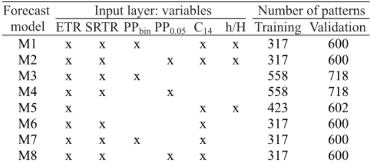
Eight models of NN of the multilayer feed-forward preceptron type were designed. All of them included three neuron layers, input, hidden and output layer (Figure 1). Each model was built with a different number of neurons in the input layer (Ei) (Table 1),
which received as input patterns, the following daily values: extraterrestrial radiation (ETR, in MJ m-2 d-1),
which is calculated on the basis of latitude and the day of the year, according to Chassériaux (1990), and considers a solar constant of 1,370 W m-2, adjusted
by the earth’s position; square root of the temperature
range (SRTR, ºC½), following the procedure used by Liu
& Scott (2001). The precipitation was considered in two different ways, as a potential function with exponent 0.05 (PP0.05, mm0.05), according to Alonso
et al. (2002), and as a binary function with value 1 for occurrence and zero for days with no precipitation (PPbin)
(Liu & Scott, 2001). This representation does not mean an important loss of information, since according to our data, in 95% of the cases with precipitation, the values of the potential function differ from the unit in less than 0.15; cloudiness observed at 14 hours local time (C14 oktas) and the relative sunshine duration (h/H%, in
which h is the sunshine duration, and H is the day duration, both in hours).
The hidden layer for all models was built with five neurons (Oj) and the output layer was built with only one neuron (S) that indicates the daily estimated solar radiation (SR, in MJ m-2 d-1).
Records of this meteorological information for the period 1988/1991 were taken from the Córdoba Observatory Station, in Argentina (31º26'S; 64º11'W; 438 m), which belongs to the Servicio Meteorológico Nacional (SMN). The global daily solar radiation data for the same period were supplied by the Centro de Investigaciones Acústicas y Luminotécnicas (Cial) (31º26'S; 64º11'W; 549 m), which belongs to the Red Solimétrica Nacional of the Universidad Nacional de Córdoba.
The steps that demonstrate the training algorithm of the proposed networks are described, according to Hilera & Martínez (2000), as follows: initialise the weights in the net with random values (step 1); read an input pattern Xp: (xp1, xp2, ..., xpN) and the desired
w1,1
w5,5
w5
w1
E1
E5 O5
O1
S ETR
SRTR
PPbin E3
E2
O4
O2
O3
E4
C14
h/H
output d: (d1, d2, ..., dM) associated to such input,
corresponding to the records of the years 1988/1989 (step 2); generate the output calculated by the net for the presented input. To do so, the values of the answers in each layer are obtained, until the output layer is reached (step 3). The sub-steps to be followed are described in the next paragraphs.
The net for the hidden neurons coming from the input (net) is calculated. For a hidden neuron j (Oj):
,
in which p is the p-th training vector; j is the j-th hidden neuron; wji is the weight of the connection between Ei
and Oj; and θj is the minimum threshold to be achieved
by the neuron for its activation. Based on these inputs, the outputs of the hidden neurons (y) are calculated, using the sigmoid activation function f to minimise the error:
. To obtain the results of each k neuron in the output layer, the same is done:
.
Once all neurons have an activation value for a given input pattern, the algorithm continues calculating the error for each neuron, except for those in the input layer (step 4). For the k neuron in the output layer, if the answer is (y1, y2, ..., yM), such error (δ) can be
expressed as , and for the
sigmoid function in particular: δpk = (dpk - ypk)ypk (1 - ypk).
If the neuron j is not an output one, then the partial derivative of the error cannot be directly calculated. Thus, the result is obtained out of known values and others that can be evaluated. The resulting formula is:
,
in which the error in the hidden layers depends on all the terms of the error in the output layer. For this reason they are called backpropagation.
The error in a hidden neuron is proportional to the sum of the known errors that are produced in the neurons connected to its output, each of them multiplied by the weight of the connection. The inner thresholds for the neurons are adapted in a similar way, considering they are connected with weights from auxiliary inputs with constant value.
In order to update the weights, a recursive algorithm is used, starting with the output neurons and working backwards until the input layer is reached (step 5). These weights are adjusted in the output layer neurons as
; and in the hidden layer
neurons as ;
.
In both cases, to accelerate the learning process, a learning rate (α) equal to 1 is included, and to correct the direction of the error, a moment term γ
(
wkj(t) - wkj(t - 1))
is used in the case of an output neuron, and
γ
(
wji(t) - wji(t - 1))
when it is the case of a hiddenlayer, with a γ rate equal to 0.7.
This process is repeated an n number of times, so that an acceptably low square error (Ep) for all the
learned patterns can be reached (step 6):
.
In this learning phase of the designed net, a thousand repetitions were done to ensure that the minimum square error was less than 0.01.
The model validation phase was done with the weights generated in this first stage, and the registered data of the years 1990/1991. The number of records for each model can be observed in Table 1.
Input layer: variables Number of patterns
Forecast
model ETR SRTR PPbinPP0.05 C14 h/H Training Validation
M1 x x x x x 317 600
M2 x x x x x 317 600
M3 x x x 558 718
M4 x x x 558 718
M5 x x x 423 602
M6 x x x 317 600
M7 x x x x 317 600
M8 x x x x 317 600
Results and Discussion
The results of the validation process of all models allowed the calculation of different statistic values of the error and the correlation coefficient between observed and estimated values of solar radiation for Córdoba (Table 2). All models present good performance in the estimation of solar radiation.
The results of the models that, using the same input, differ only in the consideration of precipitation (M1 and M2; M3 and M4; M7 and M8) show a similar behaviour; therefore, in weather stations where rainfall is not measured, the occurrence or absence of the phenomenon can be used without any loss in the quality of radiation estimation.
In cases of no data on sunshine duration, the records of cloudiness at 14 hours become relevant in the estimation of solar radiation, as shown in models M6, M7 and M8. The models that consider only temperature and precipitation information (M3 and M4) are the ones which show greater errors in the estimation. However, this difference is not relevant.
In order to analyse the performance of the models that present better adjustment (M1 and M2), a dispersion diagram considering observed and estimated solar radiation values was done in the validation stage of model M1 (Figure 2). This model tends to underestimate the highest values of observed solar radiation. For daily radiation over 25 MJ m-2 d-1 the underestimation
percentage reaches, on average, 15%.
In the analysed models, the temporal evolution of the estimated values of solar radiation shows a seasonal behaviour pattern correctly adjusted to those of observed ones. As an example, Figure 3 shows the temporal evolution for the model M1. The maximum values
obtained in it tend to underestimate the real ones. This becomes more apparent during summer.
The results of the models agree with similar researches on the estimation of solar radiation. Both Liu & Scott (2001) and Podestá et al. (2004) observed that the models considering precipitation as a binary variable had a similar result compared to those which used rainfall data (mm) as an input.
The results obtained applying different neural networks show similar values to those found previously. Liu & Scott (2001) estimated solar radiation in different cities in Australia using temperature and precipitation data. Their root mean square error (RMSE) values were between 2.01 and 5.44 MJ m-2 d-1.
The comparison of the results for different models proves that the exclusion of sunshine duration as a relative variable increases the error and reduces the correlation coefficient in the validation stage.
Table 2. Root mean square error (RMSE), mean absolute error (MAE), and linear correlation coefficient (r) in the validation phase for the different models.
RMSE MAE
Model
(MJ m-2d-1
r
M1 3.15 2.37 0.92
M2 3.14 2.37 0.92
M3 3.87 2.90 0.86
M4 3.88 2.91 0.86
M5 3.16 2.35 0.91
M6 3.30 2.49 0.90
M7 3.30 2.49 0.90
M8 3.30 2.50 0.90
--- )
---Figure 3. Evolution of observed and estimated solar radiation in Córdoba, Argentina (Model M1).
Figure 2. Relationship between observed and estimated so-lar radiation in Córdoba, Argentina (Model M1).
0 5 10 15 20 25 30 35
1 60 119 178 237 296 355 414 473 532 591 Day
Ra
dia
tio
n
v
al
ue
(M
J
m
-2
d
-1)
Different authors also noted the importance of sunshine duration in the estimation of solar radiation. Alonso et al. (2002) found a higher root mean square error in the estimation of solar radiation, for different locations in Argentina, when a model based on temperature range and daily precipitation was used. This error is higher than the one found by the Angström-Prescott traditional method, that uses relative sunshine duration as input data. The average values of RMSE were 2.55 MJ m-2 d-1 when sunshine duration was used,
and increased to 3.87 MJ m-2 d-1, when temperature and
precipitation were used.
Podestá et al. (2004) reported an average RMSE of 1.72 MJ m-2 d-1 for the Pampa Húmeda in Argentina,
with estimations based on relative sunshine duration. When using temperature and precipitation, such errors reached an average of 3.76 MJ m-2 d-1. The values of
the correlation coefficient decreased from 0.98 to 0.90, respectively (Table 2).
When calculating solar radiation in Córdoba on the basis of relative sunshine duration and cloudiness, de la Casa et al. (2003) found RMSE of 3.60 and 3.13 MJ m-2 d-1,
respectively. The error increased to 3.74 MJ m-2 d-1,
when temperature range was used, and to 3.82 MJ m-2 d-1,
when a second degree function of precipitation was considered.
Even if the errors are slightly higher, it is very important to consider the M3 and M4 models, which use only temperature and precipitation as input, since in Argentina, most of the stations have only instruments to measure these variables; these models constitute then a very useful tool.
Conclusions
1. The modelling process using neural networks is effective to estimate solar radiation, when only a limited number of meteorological variables is available.
2. These models allow the adjusted reproduction of the patterns of the temporal evolution of solar radiation.
3. The results of the models that differ only in the way the rainfall is considered, show a similar behaviour; the models considering only temperature and precipitation information are the ones that show greater errors in the estimation; however, this difference is not relevant.
References
ALEXIADIS, M.C.; DOKOPOULOS, P.S.; SAHSAMANOGLOU, H.S.; MANOUSARIDIS I.M. Short-term forecasting of wind-speed and related electrical-power. Solar Energy, v.63, p.61-68, 1998.
ALONSO, M.R.; RODRÍGUEZ, R.O.; GÓMEZ, S.G.; GIAGNONI, R.E. Un método para estimar la radiación global con la amplitud térmica y la precipitación diarias. Revista de la Facultad de Agronomía de la Universidad de Buenos Aires, v.22, p.51-56, 2002.
BALL, R.A.; PURCELL, L.C.; CAREY, S.K. Evaluation of solar radiation prediction models in North America. Agronomy Journal, v.96, p.391-397, 2004.
BENVENUTO, F.; MARANI, A. Neural networks for environmental problems: data quality control and air pollution nowcasting. Global Nest: the International Journal, v.2, p.281-292, 2000.
BOCCO, M.; SAYAGO, S.; TÁRTARA, E. Elección de alternativas productivas en explotaciones hortícolas: modelización a partir de la programación multiobjetivo. Investigación Agraria: Producción y Protección Vegetales, v.15, p.27-46, 2000.
BOOTE, K.J.; JONES, J.W.; PICKERING, N.B. Potential uses and limitations of crop models. Agronomy Journal, v.88, p.704-716, 1996.
BRAHM, B.; VARAS, C.E. Disminución de los tiempos de entrenamiento en redes neuronales artificiales aplicadas a hidrología. Ingeniería Hidráulica en México, v.18, p.69-82, 2003.
CHASSÉRIAUX, J.M. Conversión térmica de la radiación solar. Buenos Aires: Librería Agropecuaria, 1990. 306p.
CLAIR, T.A.; EHRMAN, J.M. Using neural networks to assess the influence of changing seasonal climates in modifying discharge, dissolved organic carbon, and nitrogen export in eastern Canadian rivers. Water Resources Research, v.34, p.447-455, 1998. DE JONG, R.; STEWART, D.W. Estimating global solar radiation from common meteorological observations in western Canada. Canadian Journal of Plant Science, v.73, p.509-518, 1993. DE LA CASA, A.; OVANDO, G.; RODRÍGUEZ, A. Estimación de la radiación solar global en la provincia de Córdoba, Argentina, y su empleo en un modelo de rendimiento potencial de papa. Revista de Investigaciones Agropecuarias, v.32, p.45-61, 2003.
ELIZONDO, D.; HOOGENBOOM, G.; McCLENDON, R.W. Development of a neural network model to predict daily solar radiation. Agricultural and Forest Meteorology, v.71, p.115-132, 1994.
GROSSI GALLEGOS, H. Distribución de la radiación solar global en la República Argentina. II. Cartas de radiación. Energías Renovables y Medio Ambiente, v.5, p.33-42, 1998.
MOHANDES, M.A.; REHMAN, S.; HALAWANI, T.O. A neural networks approach for wind speed prediction. Renewable Energy, v.13, p.345-354, 1998b.
MOHANDES, M.A.; REHMAN, S.; HALAWANI, T.O. Estimation of global solar radiation using artificial neural networks. Renewable Energy, v.14, p.179-184, 1998a.
NJAU, E.C. A new analytical model for temperature predictions. Renewable Energy, v.11, p.61-68, 1997.
NOIA, M.; RATTO, C.F.; FESTA, R. Solar irradiance estimation from geostationary satellite data. I. Statistical models. Solar Energy, v.51, p.449-456, 1993a.
NOIA, M.; RATTO, C.F.; FESTA, R. Solar irradiance estimation from geostationary satellite data. II. Physical models. Solar Energy, v.51, p.457-465, 1993b.
PODESTÁ, G.P.; NÚÑEZ, L.; VILLANUEVA, C.A.; SKANSI, M.A. Estimating daily solar radiation in the Argentine Pampas.
Agricultural and Forest Meteorology, v.123, p.41-53, 2004. REDDY, K.S.; RANJAN, M. Solar resource estimation using artificial neural networks and comparison with other correlation models. Energy Conversion and Management, v.44, p.2519-2530, 2003.
SHAMSELDIN, A.Y. Application of a neural network technique to rainfall-runoff modelling. Journal of Hydrology, v.199, p.272-294, 1997.
TOVAR, H.F.; BALDASANO, J.M. Solar radiation mapping from NOAA AVHRR data in Catalonia, Spain. Journal of Applied Meteorology, v.40, p.1821-1834, 2001.
WEISS, A.; HAYS, C.J. Simulation of daily solar irradiance. Agricultural and Forest Meteorology, v.123, p.187-199, 2004.
ZURADA, J. Introduction to artificial neural systems. Boston: PWS, 1992. 785p.