FEDERAL UNIVERSITY OF PARÁ GEOSCIENCES INSTITUTE
GRADUATE PROGRAM IN GEOPHYSICS
THESIS
Structural constraints for image-based inversion
methods
JONATHAS DA SILVA MACIEL
JONATHAS DA SILVA MACIEL
Structural constraints for image-based inversion methods
Thesis presented to Graduate Program in Geophysics of the Geosciences Institute at Federal University of Pará, in fulĄllment of the requirements for obtaining the title of Doctor in Geophysics.
Maciel, Jonathas da Silva, 1984-
Structural constraints for image-based inversion methods / Jonathas da Silva Maciel. - 2016.
Orientador: Jessé Carvalho Costa.
Tese (Doutorado) - Universidade Federal do Pará, Instituto de Geociências, Programa de Pós-Graduação em Geofísica, Belém, 2016.
1. Geofísica. 2. Equação de onda - Modelos matemáticos. 3. Método de análise de velocidade. 4. Processamento de imagens - Morfologia. I. Título.
CDD 22. ed. 550
ACKNOWLEDGMENTS
I would to thank my supervisor professor Dr. Jessé Carvalho Costa by the reli-ance, knowledge and experience passed to me, of which will be useful throughout of my professional life.
The current and previous coordinator of Graduate Program in Geophysics (GPG), Dr. Cicero Régis and Dra. Ellen Gomes, for the support and encouragement of participation of Programa de Doutorado Sanduíche no Exterior (CAPES/PDSE). Also the secretaries:
Benildes Lopes, Lucibela Cardias and Suelen Buzaglo for transforming my academic life less complicated.
To my friends: Andrei Oliveira for technical support at GPGŠs computers, Carlos Alexandre Costa, Francisco Neto, Josafat Cardoso, Wildney Vieira and Williams Lima by technical discussions about inversion methods.
I would like to thank the professor Dr. Eric Verschuur and DELPHI consortium, by opportunity of working as a visiting researcher at Delft University of Technology, Kingdom of the Netherlands, as well as the secretary Margaret van Fessem by throughout aid in Delft.
I am grateful for the Ąnancial support provided by the Compagnie Générale de Géophysique (CGG Brazil), through the cooperation agreement for the training of doctors in geophysics, applied to exploration and production of hydrocarbons (CGG-UFPA). I also thank the MEC/CAPES by participation in PDSE program. Thank to Instituto Nacional de Ciência e Tecnologia - Geofísica do Petróleo (INCT-GP) by the travel allowance in
international conferences in geophysics.
To committee members by the availability and suggestions that enrich this work.
And especially to my family: my father Elias Maciel (in memoriam) and my mother
RESUMO
Esta tese apresenta duas metodologias de regularização estrutural para os métodos de análise de velocidade com migração e inversão conjunta com migração: regularização gradiente cruzado e Ąltragem com operadores morfológicos. Na análise de velocidade com migração, a regularização de gradiente cruzado tem como objetivo vincular os contrates de velocidade com o mapa de reĆetividade, através da paralelização dos vetores gradiente de velocidade com os vetores gradiente da imagem. Propõe-se uma versão com gradiente cruzado das funções objeto de minimização: Differential Semblance,Stack Power ePartial Stack Power. Combina-se a função Partial Stack Power com sua versão de gradiente
cruzados, com o objetivo de aumentar gradativamente a resolução do modelo de velocidade, sem comprometer o ajuste das componentes de longo comprimento de onda do modelo de velocidade. Na inversão conjunta com migração propõe-se aplicar os operadores morfológicos de erosão e dilatação, no pré-condicionamento do modelo de velocidade em cada iteração. Os operadores usam o mapa de reĆetividade para delimitar as regiões com mesmo valor de propriedade física. Eles homogenizam a camada geológica e acentuam o contraste de velocidade nas bordas. Os vínculos estruturais não apenas irão reduzir a ambiguidade na estimativa do modelo de velocidade, mas tornará os métodos de inversão com migração mais estáveis, reduzindo artefatos, delineando soluções geologicamente plausíveis e acelerando a convergência da função objeto de minimização.
ABSTRACT
This thesis presents two methodologies of structural regularization for Wave-Equation Migration Velocity Analysis and Joint Migration Inversion: cross-gradient regularization and Ąltering with morphological operators. In Wave-Equation Migration Velocity Analysis, the cross-gradient regularization aims to constrain the velocity contrasts with the reĆectivity map by parallelization of the velocity gradient vector and the image gradient vector. We propose a version with cross-gradient of the objective functions: Differential Semblance, Stack Power and Partial Stack Power. We combine the Partial Stack Power with its version of cross-gradient, in order to gradually increase the resolution of the velocity model without compromising the adjustment of the long wavelengths of the velocity model. In Joint Migration Inversion, we propose to apply morphological operators of erosion and dilation in the preconditioning of the velocity model in each iteration. Operators use the reĆectivity map to mark the regions with the same value of physical property. They homogenize the geological layer and accentuate the velocity contrast at the edges. Structural constraints do not only reduce the ambiguity in estimating a velocity model, but also make the migration/inversion methods more stable, reducing artifacts, delineating geologically plausible solutions, and accelerating the convergence of the objective function.
LIST OF ILLUSTRATIONS
Figure 2.1 Ű Coordinate system. . . 22
Figure 2.2 Ű Reverse Time Migration (RTM) process: cross-correlation of forward waveĄeld (a) with backward waveĄeld (b), producing the image (c). . 23
Figure 2.3 Ű ODCIG migrated with velocity values: (a) 20% greater, (b) exact and (c) 20% smaller. . . 23
Figure 2.4 Ű ADCIG migrated with velocity values: (a) 20% greater, (b) exact and (c) 20% smaller. . . 24
Figure 2.5 Ű Stack Power (SP), Differential Semblance (DS) and Partial Stack Power (PSP) penalty operators, in ADCIG (blue) and ODCIG (red) domains. . . 26
Figure 2.6 Ű The arrows show the eigenvalues of 2.9. Higher weights along structures than across then, and equal weights inside the layers. . . 27
Figure 2.7 Ű A cross-gradient regularization parallelize the gradient vectors ∇𝑐and ∇𝐼, minimizing (maximize) their outer (inner) product in a least-square sense. . . 28
Figure 2.8 Ű Gaussian window changing the phase analysis (large) to amplitude analysis (squeezed). Note the delay between the Partial Stack Power (continuous lines) and Cross-Gradient Partial Stack Power (dashed lines), which is reduced when the background is adjusted. . . 29
Figure 2.9 Ű Velocity model. . . 32
Figure 2.10 Ű Migrated image with: . . . 33
Figure 2.11 Ű ODCIG migrated with true velocity. . . 34
Figure 2.12 Ű ODCIG migrated with initial velocity. . . 35
Figure 2.13 Ű ODCIG migrated with optimized Partial Stack Power velocity. . . 36
Figure 2.14 Ű ODCIG migrated with optimized Cross-Gradient Partial Stack Power velocity. . . 37
Figure 2.15 Ű ODCIG zero offset image traces 𝑥1 = (3000,3600,4200,4800,5400) m: true migration (blue), Partial Stack Power migration (red) and Cross-Gradient Partial Stack Power (black). . . 38
Figure 2.16 Ű ODCIG zero offset image traces 𝑥1 = (6000,6600,7200,7800,8400) m: true migration (blue), Partial Stack Power migration (red) and Cross-Gradient Partial Stack Power (black). . . 39
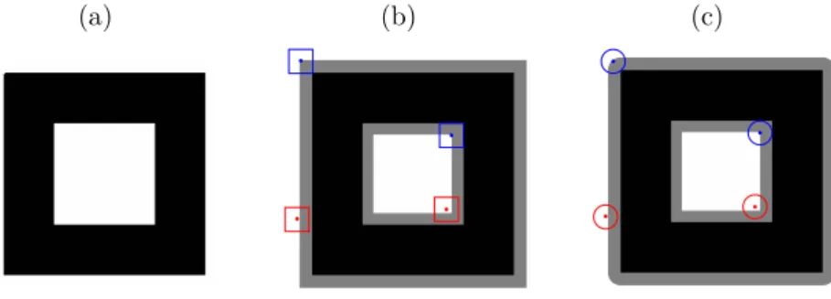
Figure 4.1 Ű Original image (a) and the results of binary erosion with (b) a square and (c) a circle structural element. The origin position of the structural element is represented as a dot, and the colors blue and red represent the match and unmatched criteria of equation (4.1), respectively. The binary eroded image (black) is created by setting the foreground pixels in all translations for which 𝐵 is totally inside of 𝐴 (i.e the gray area). 50 Figure 4.2 Ű Original image (a) and the result of binary dilation with (b) a square
and (c) a circle structural element. The origin position of the structural element is represented as a dot, and the colors blue and red represent the match and unmatched criteria of equation (4.2), respectively. The binary dilation image (gray) is created by setting the foreground pixels in all translations for which 𝐵 touches 𝐴 (black). . . 50
Figure 4.3 Ű Erosion and dilation in a 1D gray-scale function. (a) Gray-scale function𝑓(x) and Ćat null structural function𝑔(x). The dot represent
the origin of the 𝑔(x)Šs coordinate system. (b) Erosion (blue) and (c)
dilation (red). . . 52 Figure 4.4 Ű 2D morphological operators applied to a gray-scale image. . . 52 Figure 4.5 Ű Step formation: 𝑓(𝑥) masked (black), (a) Erosion (blue) and (b)
dilation (red). . . 53 Figure 4.6 Ű 1D morphological operators applied to function 𝑓(𝑥) =𝑠𝑖𝑛(𝑥) (black
curve): (a) Standard erosion (blue) and dilation (red) and the average function (magenta), for 𝑘 = 10 (dotted line),𝑘 = 30 (dashed line) and 𝑘 = 100 (continuous line). (b) Constrained curves 𝑓(𝑥)/𝐻(𝑥) (blue)
and 𝑓(𝑥)𝐻(𝑥) (red). (c) Structure-oriented erosion and dilation with
the same values of 𝑘 as in (a). . . 55 Figure 4.7 Ű Structure-oriented morphological operator example in 2D. (a) True
model, (b) true reĆectivity, (c) mask function 𝑀(x), (d) initial model
𝑓(x), (e) eroded model (𝑓 −𝑔)60(x), (f) dilated model (𝑓 ⊕𝑔)60(x)
and (g) the Ąnal solution 𝐴(x). Color bars are in m/s except the
reĆectivity model which is dimensionless. . . 56 Figure 4.8 Ű Subsurface model for JMI test. (a) True velocity model, (b) true
reĆectivity, (c) initial velocity model and (d) initial reĆectivity. Color bars are in m/s except the reĆectivity model which is dimensionless. . 58 Figure 4.9 Ű Standard JMI results. (a) ReĆectivity; (b) velocity; (c) proĄles at
𝑥= 1000 m: velocity (left), true velocity (blue), initial velocity (green) and Ąnal velocity (red); reĆectivity (right), true reĆectivity (blue) and Ąnal reĆectivity (red); (d) measured data (left) and the residual data (right). Color bars are in m/s except the reĆectivity model which is
Figure 4.10 Ű JMI results with morphological constraints. (a) ReĆectivity; (b) velocity; (c) proĄles at𝑥= 1000 m: velocity (left), true velocity (blue),
initial velocity (green) and Ąnal velocity (red); reĆectivity (right), true reĆectivity (blue) and Ąnal reĆectivity (red); (d) measured data (left), residual data (right). Color bars are in m/s except the reĆectivity model which is dimensionless. . . 60 Figure 4.11 Ű Subsurface model for JMI test. (a) True velocity model, (b) True
reĆectivity, (c) initial velocity model and (d) initial reĆectivity. Color bars are in m/s except the reĆectivity model which is dimensionless. . 62 Figure 4.12 Ű Standard JMI results. (a) ReĆectivity; (b) velocity; (c) proĄles at
𝑥= 900 m: velocity (left), true velocity (blue), initial velocity (green)
and Ąnal velocity (red); reĆectivity (right), true reĆectivity (blue) and Ąnal reĆectivity (red); (d) measured data (left), residual data (right). Color bars are in m/s except the reĆectivity model which is
dimensionless. . . 63 Figure 4.13 Ű JMI results with morphological constraints. (a) ReĆectivity; (b)
velocity; (c) proĄles at 𝑥= 900 m: velocity (left), true velocity (blue), initial velocity (green) and Ąnal velocity (red); reĆectivity (right), true reĆectivity (blue) and Ąnal reĆectivity (red); (d) measured data (left), residual data (right). Color bars are in m/s except the reĆectivity model which is dimensionless. . . 64
LIST OF TABLES
Table 2.1 Ű WEMVA objective functions: Stack Power and Differential Semblance for angle domain (blue) and offset domain (red). . . 24 Table 2.2 Ű WEMVA objective functions constrained by cross-gradient
regulariza-tion: Cross-Gradient Stack Power (CGSP) and Cross-Gradient Differ-ential Semblance (CGDS), for angle domain (blue) and offset domain (red). . . 28
LIST OF ABBREVIATIONS AND ACRONYMS
ADCIG Angle Domain Common Image Gather
CGDS Cross-Gradient Differential Semblance
CGPSP Cross-Gradient Partial Stack Power
CGSP Cross-Gradient Stack Power
CIG Common Image Gather
DS Differential Semblance
FWI Full Waveform Inversion
FWM Full WaveĄeld Migration
FWMod Full WaveĄeld Modeling
JMI Joint Migration Inversion
ODCIG Offset Domain Common Image Gather
PSP Partial Stack Power
RTM Reverse Time Migration
SP Stack Power
SUMMARY
1 INTRODUCTION . . . 16
1.1 Motivation . . . 16
1.2 WEMVA with cross-gradient regularization . . . 17
1.3 JMI method . . . 18
1.4 High resolution velocity estimation with morphological operators . . 18
1.5 General conclusions and appendices . . . 19
2 WEMVA WITH STRUCTURAL PRIOR INFORMATION . . . 20
2.1 Introduction . . . 20
2.2 WEMVA theory . . . 22
2.3 Constraining the velocity model with the reflector map . . . 26
2.4 Numerical experiments . . . 30
2.5 Conclusions . . . 40
3 JOINT MIGRATION INVERSION . . . 41
3.1 Full Wavefield Modeling . . . 41
3.2 Velocity perturbations . . . 44
3.3 Reflectivity perturbations . . . 45
3.4 Inversion . . . 45
4 ENHANCING RESOLUTION IN IMAGE-BASED VELOCITY ES-TIMATION USING MORPHOLOGICAL OPERATORS . . . 48
4.1 Erosion and dilation for binary images . . . 49
4.2 Erosion and dilation for gray-scale images . . . 51
4.3 Enhancing the sharpness with modified erosion and dilation operators 53 4.4 Application of morphological operators in the JMI method . . . 57
4.4.1 2D simple model with strong internal multiples . . . 57
4.4.2 2D complex model with strong internal multiples . . . 61
4.5 Conclusion . . . 65
5 GENERAL CONCLUSIONS . . . 66
Bibliography . . . 68
16
1 INTRODUCTION
1.1
Motivation
Tomographic methods based on ray tracing are well established in the oil industry as the main tool for velocity model building. The velocity model is estimated in order to optimize focusing of selected reĆection events. As a consequence tomographic velocity models produce good images of the subsurface, but require intense human interaction for event selection and editing. Another well known limitation of tomographic methods results from the high-frequency approximation to describe wave propagation, which limits these methods to regions of mild geological complexity. Currently there are several efforts to develop velocity model building methods that do not have the limitations of ray methods and can take advantage of more accurate descriptions of the waveĄeld.
Wave-equation based inversion can be divided into three branches: inversion meth-ods with objective function speciĄed in the data domain as Full Waveform Inversion [FWI, (VIRIEUX; OPERTO, 2009)], inversion methods with objective function deĄned in the image domain as Wave-Equation Migration Velocity Analysis [WEMVA, (SAVA; BIONDI, 2004)] and hybrid inversion methods like Joint Migration Inversion [JMI, (BERKHOUT, 2014a; BERKHOUT, 2014b; BERKHOUT, 2014c)]. In the latter approach, the model parameterization is extended to include a background velocity and a reĆectivity model. The velocity model is estimated from Ątting the waveĄeld spectrum and reĆectivity from least-squares migration. The objective function in FWI minimizes the difference between the modeled and recorded traces. WEMVA uses migration methods to generate Common Image Gathers (CIG), where an objective function will measure the focusing. JMI, like FWI, minimizes the differences between modeled data and recorded data, but differently from FWI, JMI separates the waveĄeld-phase Ątting, to estimate the velocity model, and the waveĄeld-amplitude Ątting to estimate the reĆectivity of subsurface.
Chapter 1. INTRODUCTION 17
WEMVA and JMI, like many other non-linear inverse-problem methods, need preconditioning or regularization to ensure stability and reduce the ambiguity in inversion. Traditionally smoothness constraints, such as Tikhonov regularization (TIKHONOV; ARSENIN, 1977; KAIPIO et al., 1999; WEIBULL; ARNTSEN, 2013), are used to stabilize inversion in wave-equation velocity-model building. WEMVA and JMI have in common the estimation of a migrated image or reĆectivity model during the inversion. These images can be used as prior information to increase the resolution of the velocity model.
This thesis aims at developing techniques to increase the velocity model resolution of inversion methods in the image domain. The techniques of preconditioning and reg-ularization do not only reduce the ambiguity of optimized solutions, but, as suggested by Williamson et al. (2011), the use of structural regularization also adds geologically meaningful information to the model. Moreover, preconditioning also speeds up the convergence of the method. Another aspect I explore is the variation of the regularization parameter during the iterations. At initial iterations smoothness constraints are enforced to help the recovering of long wavelength components of the velocity model. Structural information is gradually enforced at later iterations to avoid the inversion to be trapped prematurely in local minima far from the optimal solution. The following sections present the regularization techniques based in structural constraints and the organization of this thesis.
1.2
WEMVA with cross-gradient regularization
Chapter 1. INTRODUCTION 18
contrast normal to reĆectors, by aligning the velocity gradient vector with the migrated image-gradient vector in a least-square sense. The product of Partial Stack Power with cross-gradient regularization is proposed to enforce structural information. Using this multiplicative objective function, the structural regularization can be introduced gradually without compromising convergence. This new formulation of WEMVA is validated on Marmousoft data set.
1.3
JMI method
Chapter 3 presents the JMI method for isotropic media with no dependence on angle for the reĆectivity model (STAAL; VERSCHUUR, 2014). JMI uses the one-way wave equations to separately modeling downgoing and upgoing waveĄelds. This feature enables a greater control over multiples, allowing JMI to generate, through least-squares migration, high-resolution reĆectivity maps without preprocessing to attenuate multiples in the data. Another positive feature of one-way modeling is the separation of phase and amplitude of the waveĄeld. The velocity estimation is correlated with the perturbation of the waveĄeld extrapolation phase-shift operator, while the reĆectivity model is estimated from waveĄeld amplitudes. This approach makes the problem much better conditioned. The chapter Ąnalizes presenting the derivation of velocity and reĆectivity gradients used in the optimization and the description of the JMI inversion algorithm.
1.4
High resolution velocity estimation with morphological operators
Chapter 1. INTRODUCTION 19
1.5
General conclusions and appendices
20
2 WEMVA WITH STRUCTURAL PRIOR
INFORMA-TION
Wave-Equation Migration Velocity Analysis (WEMVA), like many other geophysical inversion methods, needs extra information to reduce the ambiguity in its solutions. However, unlike other methods, WEMVA has the advantage of having at its disposal the migrated image, from where we can extract structural information, allowing to get a well Ątted model with subsurface geology. Using the concept of cross-gradient, this work proposed to couple the WEMVA objective function called Partial Stack Power, which combines the Differential Semblance and Stack Power, with its analogous version with cross-gradient, to precondition WEMVA convergence and increase the velocity model information.
2.1
Introduction
Methods using wave-equation modeling represent the best tools to image regions with complex geology, because they do not suffer from limitations in wave simulation, including information like refraction, diffraction, primaries and multiples. The evaluation of all these information is well computed in inversion methods in the data domain like Full Waveform Inversion [FWI, (VIRIEUX; OPERTO, 2009)]. FWI is gaining importance by producing better and detailed velocity models. Unfortunately FWI hardly converges if the low frequency, inside of the data and inside of the model, are not well Ątted. However Wave-Equation Migration Velocity Analysis [WEMVA, (SAVA; BIONDI, 2004)], an image based inversion method, has less sensitivity to the initial model, also has the advantage of working with the frequency band conventionally acquired in seismic experiments, and it does not require large offsets to estimate the model in deeper regions as does FWI.
Improve the WEMVA method is a valid objective to enrich the toolbox of inversion methods in geophysics. For this purpose, it is necessary to highlight one the main negative features of the WEMVA method: the presence of strong artifacts in the objective function gradient (FEI; WILLIAMSON, 2010). These artifacts usually dominate the useful gradient and increase the optimization time.
Chapter 2. WEMVA WITH STRUCTURAL PRIOR INFORMATION 21
have cover all offsets, in this case the zero-offset amplitude maximization is not evaluated. The Stack Power (SP) function can be included in Differential Semblance optimization to supply the zero-offset amplitude correction (CHAVENT; JACEWITZ, 1995; WEIBULL; ARNTSEN, 2013).
Zhang and Shan (2013) noted that the difference between Differential Semblance and Stack Power, is the kind of weight function that is convolved with the Common Image Gather (CIG). In the angle domain Differential Semblance is equivalent to the convolution of Ąnite-difference operator with the CIG, while Stack Power represents the convolution of the CIG with the constant 1. A Radon transform (Fourier transform for plane waves) changes these convolutions to a multiplication with the offset-vector norm, ♣h♣, and the Dirac delta Ó(h), respectively. This analysis suggests the possibility to evaluate Stack Power locally like Differential Semblance (MACIEL; COSTA; SCHLEICHER, 2012). The idea is to stack the image traces in a small Gaussian window, bringing to Stack Power better convergence proprieties as Differential Semblance, with advantage to compute the zero-offset amplitude residual. They named this new objective function as Partial Stack Power (PSP).
There is additional zero offset information which can help to conditioning WEMVA. It is the application of structure-oriented Ąlters (FEHMERS; HÖCKER, 2003). Using an approximation of the anisotropic diffusion equation, as shown by Hale (2009), Williamson et al. (2011) smoothed the objective function gradient. They showed that in this way the velocities models recovered the main features of true velocity. Moreover this procedure accelerated the methodŠs convergence. However it implied in resolving one more linear system per iteration.
Chapter 2. WEMVA WITH STRUCTURAL PRIOR INFORMATION 22
2.2
WEMVA theory
In this work, I assume that wave propagation is described by the acoustic equation with constant density,
2𝑃(x, 𝑡)⊕
[︃
1
𝑐2(x)
𝜕2
𝜕𝑡2 ⊗ ∇ 2
⟨
𝑃(x, 𝑡) = 𝐹(x, 𝑡), (2.1)
where2 is the wave equation operator,𝑐(x) is the wave velocity, 𝑃(x, 𝑡) the pressure Ąeld,
𝐹(x, 𝑡) the seismic source, x = (𝑥1, 𝑥2, 𝑥3) a subsurface position (Figure 2.1) and 𝑡 the
time instant.
Figure 2.1 – Coordinate system.
Source: By the author
According to Claerbout (1971), a migrated image, 𝐼(x), is made by the cross-correlation between the downward wave Ąeld 𝐷(x, 𝑡, 𝑠) (source Ąeld) with the upward wave Ąeld 𝑈(x, 𝑡, 𝑟) (receiver Ąeld), modeled with recorded traces injected from the last
sample to the Ąrst,
𝐼(x) =
Ns ∑︁
s=1
Nr(s) ∑︁
r=1 ∫︁ T
0 𝑑𝑡𝐷(x, 𝑡, 𝑠)𝑈(x, 𝑡, 𝑟), (2.2)
where 𝑁s is the number of shots,𝑁r(𝑠) is the number of receivers per shot and 𝑇 is the total recording time, see Figure 2.2.
If the velocity model is wrong, the Claerbout image condition, equation 2.2, will focus the energy in a wrong position. That energy can be related to a displacement of source and receiver in space (RICKETT; SAVA, 2002), in time (SAVA; FOMEL, 2006) or in space-time (YANG; SAVA, 2010). The collection of all these information is called the Offset Domain Common Image Gather (ODCIG),
𝐼(x,h, á) =
Ns ∑︁
s=1
Nr(s) ∑︁
r=1 ∫︁ T
0 𝑑𝑡𝐷(x⊗h, 𝑡⊗á, 𝑠)𝑈(x+h, 𝑡+á, 𝑟), (2.3)
where h = (ℎ1, ℎ2, ℎ3) is the sub-surface offset and á is the time shift. However, using
Chapter 2. WEMVA WITH STRUCTURAL PRIOR INFORMATION 23
Figure 2.2 – Reverse Time Migration (RTM) process: cross-correlation of forward wavefield (a) with backward wavefield (b), producing the image (c).
(a)𝐷(x, 𝑡) (b)𝑈(x, 𝑡)
(c)𝐼(x)
Source: By the author
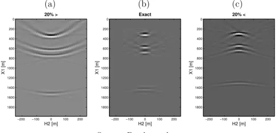
Figure 2.3 – ODCIG migrated with velocity values: (a) 20% greater, (b) exact and (c) 20% smaller.
(a) (b) (c)
20% <
H2 [m]
X1 [m]
−200 −100 0 100 200 0
200 400 600 800 1000 1200 1400 1600 1800
Exact
H2 [m]
X1 [m]
−200 −100 0 100 200 0
200 400 600 800 1000 1200 1400 1600 1800
20% >
H2 [m]
X1 [m]
−200 −100 0 100 200 0
200 400 600 800 1000 1200 1400 1600 1800
Source: By the author
Chapter 2. WEMVA WITH STRUCTURAL PRIOR INFORMATION 24
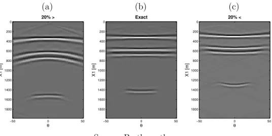
transform applied to this gather produces a Ćat horizontal event in another domain called Angle Domain Commom Image Gather (ADCIG) (BIONDI; SYMES, 2004), see Figure 2.4.
Figure 2.4 – ADCIG migrated with velocity values: (a) 20% greater, (b) exact and (c) 20% smaller.
(a) (b) (c)
20% <
θ
X1 [m]
−50 0 50
0 200 400 600 800 1000 1200 1400 1600 1800 Exact θ X1 [m]
−50 0 50
0 200 400 600 800 1000 1200 1400 1600 1800 20% > θ X1 [m]
−50 0 50
0 200 400 600 800 1000 1200 1400 1600 1800
Source: By the author
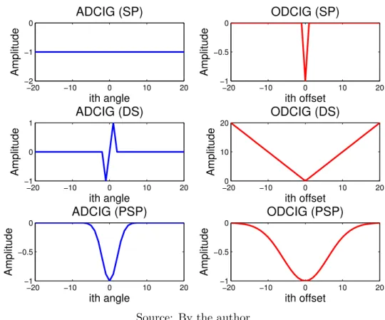
In ADCIG domain, Differential Semblance optimization (DS) (SYMES; CARAZ-ZONE, 1991) aims to measure the Ćatness events by minimization of a local derivative. Stack Power optimization (SP) aims to maximize the amplitude stacking. In ODCIG, Differential Semblance minimize all energy measured in non zero-offset image by linear offset penalty factor, and Stack Power aims to maximize the zero-offset image amplitude. The Table 2.1 show schematically the Stack Power and Differential Semblance objective functions in angle domain (blue) and in offset domain (red).
Table 2.1 – WEMVA objective functions: Stack Power and Differential Semblance for angle domain (blue) and offset domain (red).
Stack Power (SP) (Maximization)
Differential Semblance (DS) (Minimization)
ADCIG Φ(𝐼) =∑︁
x,θ
[𝐼(x, 𝜃)]2 Φ(
𝐼) =∑︁
x,θ
[︃ 𝑑𝐼 𝑑𝜃(x, 𝜃)
⟨2
ODCIG Φ(𝐼) = ∑︁ x
[𝐼(x,0)]2 Φ(𝐼) = ∑︁
x,h
[h𝐼(x,h)]2
Chapter 2. WEMVA WITH STRUCTURAL PRIOR INFORMATION 25
background velocity optimization and the amplitude Ąt with the high resolution of the velocity. Analogously in WEMVA we can say that Differential Semblance leads to a kind of phase driven optimization, whereas Stack Power leads to a kind of amplitude driven optimization.
Many authors (CHAVENT; JACEWITZ, 1995; WEIBULL; ARNTSEN, 2013) combine these two measures into a single objective function,
Φ(𝐼) = 1 2
∑︁
x,h
[h𝐼(x,h)]2
⊗Ò
2
∑︁
x
[𝐼(x,0)]2
, (2.4)
where the Ò parameter needs to be adjusted like a regularization. The many local minima of Stack Power suggest to choose a Ò parameter, that emphasizes the Stack Power
function, when Differential Semblance amplitude has lost its sensibility. This is a hard task without previously knowing the minimum Differential Semblance value. Even with this information, the convergence is not guaranteed because Stack Power is not totally an amplitude optimization.
Zhang and Shan (2013) noted that the difference between Stack Power and Dif-ferential Semblance is the Ąlter applied in each one. In Stack Power maximization the Ąlter constant 1 is convolved with ADCIG map along angle coordinate. By a Radon transform, this process is equivalent an application of DiracŠs delta Ó(h) in ODCIG domain.
Differential Semblance is a convolution of derivative operator in ADCIG domain. The equivalent in ODCIG domain is a offset linear penalty factor ♣h♣. Both operations can be generalized as:
Φ(𝐼) = 1
2
∑︁
x,θ
[𝑔(𝜃)*𝐼(x, 𝜃)]2 (2.5)
in an ADCIG and
Φ(𝐼) = 1 2
∑︁
x,h
[𝐺(h)𝐼(x,h)]2 (2.6)
in an ODCIG, see Figure 2.5.
Chapter 2. WEMVA WITH STRUCTURAL PRIOR INFORMATION 26
Figure 2.5 – Stack Power (SP), Differential Semblance (DS) and Partial Stack Power (PSP) penalty operators, in ADCIG (blue) and ODCIG (red) domains.
−20 −10 0 10 20 −2
−1 0
ADCIG (SP)
ith angle
Amplitude
−20 −10 0 10 20 −1
−0.5 0
ODCIG (SP)
ith offset
Amplitude
−20 −10 0 10 20 −1
0 1
ADCIG (DS)
ith angle
Amplitude
−200 −10 0 10 20 10
20
ODCIG (DS)
ith offset
Amplitude
−20 −10 0 10 20 −1
−0.5 0
ADCIG (PSP)
ith angle
Amplitude
−20 −10 0 10 20 −1
−0.5 0
ODCIG (PSP)
ith offset
Amplitude
Source: By the author
2.3
Constraining the velocity model with the reflector map
Is very common to conditioning a ill-posed problem with the Tikhonov regularization (TIKHONOV; ARSENIN, 1977). The Tikhonov regularization minimizes the problem
according to
arg min Φreg = Φ +Ú♣♣Γ(𝑐⊗𝑐0)♣♣2, (2.7)
where Γ is the Tikhonov differential operator, 𝑐0 is a prior velocity model and Ú the
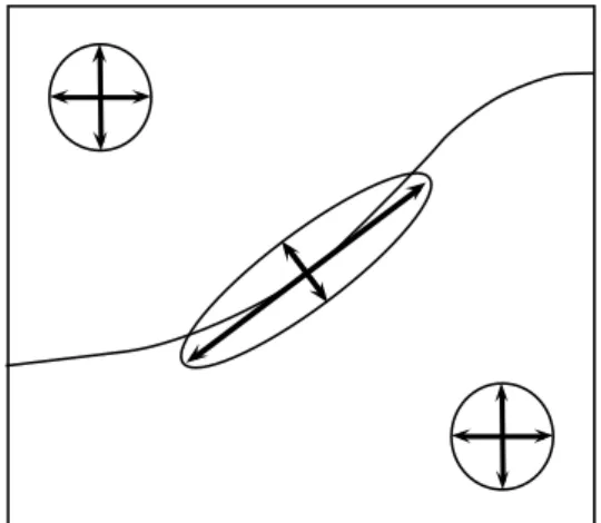
regularization parameter. It is possible to impose different conditions to the solutions, as the minimum norm, Γ⊕1, the isotropic smoothness, Γ ⊕ ∇, or the gradient condition, Γ⊕ ∇2.
Anisotropic smoothness conditions can be applied by general Tikhonov regularization,
𝑅 =Ú[∇(𝑐⊗𝑐0)]T L∇(𝑐⊗𝑐0), (2.8)
whereL is a symmetric weight matrix. For structural regularization according to Kaipio et al. (1999), L must produce an anisotropic smoothness giving smaller penalties across
discontinuities than along the faults and at places with no discontinuity the weight act isotropically, see Figure 2.6. Kaipio et al. (1999) chosen as
L=I⊗(1 +♣∇𝐼♣2)⊗1
Chapter 2. WEMVA WITH STRUCTURAL PRIOR INFORMATION 27
Figure 2.6 – The arrows show the eigenvalues of 2.9. Higher weights along structures than across then, and equal weights inside the layers.
Source: By the author
where Ithe identity matrix andS=∇𝐼(∇𝐼)T is the structure tensor.
Analyzing equation 2.9, removing the normalization and the isotropic term, I get
L=♣∇𝐼♣2I⊗S=MTM, (2.10)
with
M=
∏︀
̂︁ ̂︁ ̂︁ ̂︁ ̂︁ ̂︁ ̂︁ ̂︁ ̂︁ ∐︁
0 ∂I
∂x3 ⊗ ∂I ∂x2
⊗ ∂I ∂x3 0
∂I ∂x1
∂I ∂x2 ⊗
∂I ∂x1 0
∫︀
̂︂ ̂︂ ̂︂ ̂︂ ̂︂ ̂︂ ̂︂ ̂︂ ̂︂ ̂︀
. (2.11)
Identity 2.10 is the cross-gradient factor in Kaipio et al. (1999) regularization,
(∇𝑐)T L∇𝑐= (M∇𝑐)T (M∇𝑐)⊕ ♣∇𝐼× ∇𝑐♣2. (2.12)
The last term of 2.10 is the cross-gradient version of the inner product,
(∇𝑐)T
S∇𝑐= (∇𝑐)T
∇𝐼(∇𝐼)T
∇𝑐⊕(∇𝐼≤ ∇𝑐)2
. (2.13)
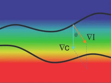
An interpretation of cross-gradient optimization is show in Figure 2.7. The Ągure shows two black curves indicating the image/reĆectivity map embedded in a linear vertical gradient velocity. When the velocity model is almost adjusted, the WEMVAŠs image update has few changes. From now, the objective function decrease manly by changing the ∇𝑐(x) direction towards the ∇𝐼(x) direction. Parallelizing the gradient vectors can
be done by minimization (maximization) of their outer (inner) product in a least-square sense.
Chapter 2. WEMVA WITH STRUCTURAL PRIOR INFORMATION 28
Figure 2.7 – A cross-gradient regularization parallelize the gradient vectors ∇𝑐 and∇𝐼, minimi-zing (maximize) their outer (inner) product in a least-square sense.
q
ID
D
c
D
c
IDexp[- ²] ~ 0
ID
exp[- ²] = 1
ID
D
c
*ID
*I D x1 *I D x3 D x1c D x3cSource: By the author
Table 2.2 – WEMVA objective functions constrained by cross-gradient regularization: Cross-Gradient Stack Power (CGSP) and Cross-Cross-Gradient Differential Semblance (CGDS), for angle domain (blue) and offset domain (red).
CG Stack Power (CGSP) (Maximization)
CG Differential Semblance (CGDS) (Minimization)
ADCIG Φ(𝐼, 𝑐) =∑︁
x,θ
[∇𝐼(x, 𝜃)≤ ∇𝑐(x)]2 Φ(𝐼, 𝑐) = ∑︁
x,θ ⧹︃ ⧹︃ ⧹︃ ⧹︃ ⧹︃ 𝑑
𝑑𝜃∇𝐼(x, 𝜃)× ∇𝑐(x) ⧹︃ ⧹︃ ⧹︃ ⧹︃ ⧹︃ 2
ODCIG Φ(𝐼, 𝑐) = ∑︁
x
[∇𝐼(x,0)≤ ∇𝑐(x)]2 Φ(
𝐼, 𝑐) =∑︁
x,h
♣h♣2♣∇𝐼(x,h)× ∇𝑐(x)♣2
The same construction can be done for the Partial Stack Power. Following the normalization proposed by Zhang and Shan (2013), the Cross Gradient Partial Stack Power in an ODCIG is deĄned as:
å(𝐼, 𝑐) = 1 2 ∑︁ x2 ∑︀ x1,h2 [︁ ˜
𝐺(h)∇𝐼(x,h)≤ ∇𝑐(x)]︁2
∑︀
x1,h2[∇𝐼(x,h)≤ ∇𝑐(x)]
2 . (2.14)
A cross-gradient objective function optimization brings high-frequency information to the velocity. It is not appropriated to apply it if the background velocity model is not solved yet. To include the cross-gradient from the beginning, it is necessary to couple it with a standard optimization function. Here, I combine the Zhang and Shan (2013) function
𝜙(𝐼) = 1 2
∑︁
x2
∑︀
x1,h2[𝐺(h)𝐼(x,h)]2
∑︀
x1,h2[𝐼(x,h)]
2 (2.15)
Chapter 2. WEMVA WITH STRUCTURAL PRIOR INFORMATION 29
use for the Cross-Gradient Partial Stack Power function the deĄnition
Φ(𝐼, 𝑐) = 𝜙(𝐼)å(𝐼, 𝑐). (2.16)
The gradient of equation 2.16 is calculated in Appendix A.
The Gaussian weights are deĄned as:
𝐺(h) = exp(⊗Ðℎ22/𝐻2), (2.17a)
˜
𝐺(h) = exp(⊗Ñℎ22/𝐻2), (2.17b)
where 𝐻 is the maximum sub-surface offset, and Ð and Ñ are parameters for squeezing
the Gaussian. Mathematically ˜𝐺 is independent of 𝐺, and in principal, choosingÐ andÑ
is as undetermined as Ú in Tikhonov regularization. However some conditions need to be
taken into account: Ð starts with a small value [wide 𝐺(h)] to include the most unfocused
energy. As the inversion proceeds, and the gathers become more focused, Ð is gradually
increased [small 𝐺(h)] to approach the Stack Power analysis (ZHANG; SHAN, 2013). For
the Ąrst iterations, the Ñ value needs to give priority to𝜙 in order to estimate estimate the background velocity. As the inversion proceeds, the weights for 𝜙 andå must approach each other asymptotically (see Figure 2.8). One suggestion is to take Ñ =Ð(1.0⊗Ð0/Ð),
where Ð0 (Ð ⊙Ð0) is the Ąrst Ð selected.
Figure 2.8 – Gaussian window changing the phase analysis (large) to amplitude analysis (squeezed). Note the delay between the Partial Stack Power (continuous lines) and Cross-Gradient Partial Stack Power (dashed lines), which is reduced when the background is adjusted.
−600 −400 −200 0 200 400 600
0 0.2 0.4 0.6 0.8 1
H2 [m]
G(H2)
α = 1.0 α = 3.0 α = 7.0 α = 20.0 β = 0.0 β = 2.0 β = 6.0 β = 19.0
Chapter 2. WEMVA WITH STRUCTURAL PRIOR INFORMATION 30
2.4
Numerical experiments
To validate the Cross-Gradient Partial Stack Power I used synthetic data from a smoothed version of the Marmousi data (VERSTEEG; GRAU, 1991) called Marmousoft (BILLETTE et al., 2003). It is a simulated marine acquisition with 261 shots and a streamer with 96 receivers. The data was modeled using the Born approximation, which means that it contains no multiples or refracted waves. The pulse is a Ricker wavelet with peak frequency of 12 Hz.
The model possesses 243 samples in the𝑥1 and 767 in the𝑥2 direction, both spaced
at 12 m. The velocities vary between 1500 m/s and 4750 m/s. Figure 2.9a shows the true velocity model.
The objective function gradient was calculated by adjoint state method (PLESSIX, 2006), see Appendix A. For optimization process I used the quasi-Newton algorithm L-BFGS-B (BYRD et al., 1995), see Appendix B. The numbers of parameters was reduced by B-splines interpolation, see Appendix C. The interpolated model has 37 samples in the
𝑥1 and 97 samples in the 𝑥2 direction, spaced at 81 m and 95.875 m respectively. The
initial model is a linear vertical gradient with velocity varying between 1500 m/s and 4500 m/s (see Figure 2.9b). The maximum subsurface offset is equal to 624 m. The optimization took 4 steps with 15 iterations each. At each step, Ð was increased empirically, taking the
values 1.0,3.0,7.0 and 20.0 (Figure 2.8).
Figure 2.9c show the model resulting from Partial Stack Power optimization. It is a model with little change with respect of the initial model, but enough to produce a well focused image (Figure 2.10c). Figure 2.9d show the velocity model build with Cross-Gradient Partial Stack Power optimization. We can note the cross-gradient regularization gives a structural information similar founded in true velocity model (Figure 2.9a), and less artifacts when we compare the region above 𝑥1 = 800 m between 𝑥2 = 6600 m and
𝑥2 = 8400 m, in Figures 2.9c and 2.9d. The correspondent PSP and CGPSP migrated
images are show in Figures 2.10c 2.10d respectively. In both cases we can see good convergence, when we compare the migrated image using the true velocity model (Figure 2.10a), and initial model (Figure 2.10b), but for CGPSP we note a better deĄnition of the layers on the region above 𝑥1 = 800 m between 𝑥2 = 6600 m and 𝑥2 = 8400 m.
Chapter 2. WEMVA WITH STRUCTURAL PRIOR INFORMATION 31
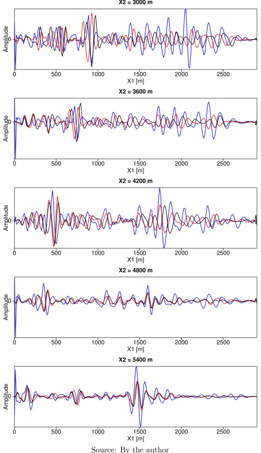
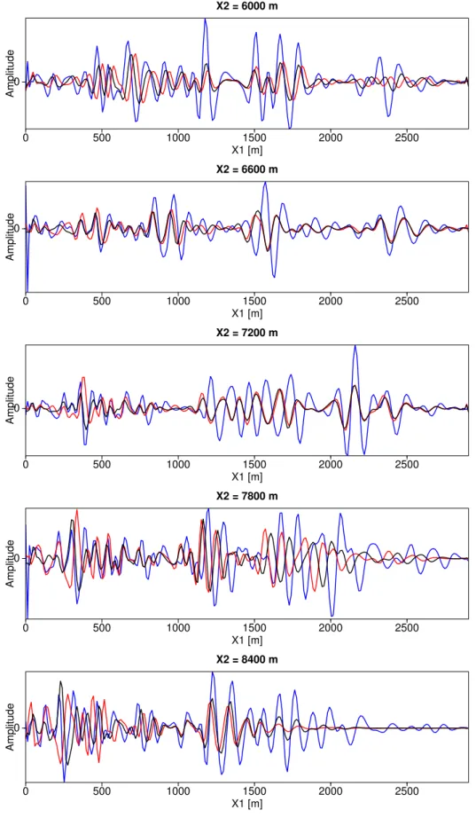
The short wavelength components of the velocity model are related with amplitude maximization in zero-offset image. The Figures 2.15 and 2.16 show the zero-offset image trace took at the CIG position mentioned above. Particularly at the positions around the target, 𝑥2 = 6000 m, 𝑥2 = 6600 m and 𝑥2 = 7200 m (the target depth is 𝑥1 = 2400 m).
Chapter
2.
WE
MV
A
WI
TH
STR
U
CTU
R
A
L
P
R
IOR
IN
F
OR
MA
TI
ON
32
Figure 2.9 – Velocity model.
(a) True (b) Initial
(c) Partial Stack Power (d) Cross-Gradient Partial Stack Power
Chapter
2.
WE
MV
A
WI
TH
STR
U
CTU
R
A
L
P
R
IOR
IN
F
OR
MA
TI
ON
33
Figure 2.10 – Migrated image with:
(a) true velocity (b) initial velocity
(c) Partial Stack Power velocity (d) Cross-Gradient Partial Stack Power velocity.
Chapter
2.
WE
MV
A
WI
TH
STR
U
CTU
R
A
L
P
R
IOR
IN
F
OR
MA
TI
ON
34
Figure 2.11 – ODCIG migrated with true velocity.
Chapter
2.
WE
MV
A
WI
TH
STR
U
CTU
R
A
L
P
R
IOR
IN
F
OR
MA
TI
ON
35
Figure 2.12 – ODCIG migrated with initial velocity.
Chapter
2.
WE
MV
A
WI
TH
STR
U
CTU
R
A
L
P
R
IOR
IN
F
OR
MA
TI
ON
36
Figure 2.13 – ODCIG migrated with optimized Partial Stack Power velocity.
Chapter
2.
WE
MV
A
WI
TH
STR
U
CTU
R
A
L
P
R
IOR
IN
F
OR
MA
TI
ON
37
Figure 2.14 – ODCIG migrated with optimized Cross-Gradient Partial Stack Power velocity.
Chapter 2. WEMVA WITH STRUCTURAL PRIOR INFORMATION 38
Figure 2.15 – ODCIG zero offset image traces 𝑥1= (3000,3600,4200,4800,5400) m: true
migra-tion (blue), Partial Stack Power migramigra-tion (red) and Cross-Gradient Partial Stack Power (black).
0 500 1000 1500 2000 2500
X1 [m] 0
Amplitude
X2 = 3000 m
0 500 1000 1500 2000 2500
X1 [m] 0
Amplitude
X2 = 3600 m
0 500 1000 1500 2000 2500
X1 [m] 0
Amplitude
X2 = 4200 m
0 500 1000 1500 2000 2500
X1 [m] 0
Amplitude
X2 = 4800 m
0 500 1000 1500 2000 2500
X1 [m] 0
Amplitude
X2 = 5400 m
Chapter 2. WEMVA WITH STRUCTURAL PRIOR INFORMATION 39
Figure 2.16 – ODCIG zero offset image traces 𝑥1= (6000,6600,7200,7800,8400) m: true
migra-tion (blue), Partial Stack Power migramigra-tion (red) and Cross-Gradient Partial Stack Power (black).
0 500 1000 1500 2000 2500
X1 [m] 0
Amplitude
X2 = 6000 m
0 500 1000 1500 2000 2500
X1 [m] 0
Amplitude
X2 = 6600 m
0 500 1000 1500 2000 2500
X1 [m] 0
Amplitude
X2 = 7200 m
0 500 1000 1500 2000 2500
X1 [m] 0
Amplitude
X2 = 7800 m
0 500 1000 1500 2000 2500
X1 [m] 0
Amplitude
X2 = 8400 m
Chapter 2. WEMVA WITH STRUCTURAL PRIOR INFORMATION 40
2.5
Conclusions
In this Chapter I discussed preconditioning WEMVA adding structural information extracted from stacked migrated images. In order to enforce the structural information we require that the gradient of the velocity Ąeld and the gradient of the image intensity are collinear. This regularization was applied as a multiplicative factor on the partial stack power objective function. The structural regularization is gradually enforced during the quasi-Newton iterations in order to avoid premature convergence to local minima. This modiĄcation resulted in velocity models correlated with the seismic image and improved the migration focusing.
The new objective function is very sensitive to high frequency noise. Preprocessing is required to attenuate multiples and coherent noises. Additionally, dynamic precondition-ing is required to decrease the nonlinearity and improve image focusprecondition-ing. In our numerical experiments we used a Gaussian Ąlter to improve the robustness when numerically com-puting of the gradients of image and velocity. A Gaussian Ąlter is used also to remove high frequency artifacts in the objective function gradient. B-splines parameterization of the velocity model reduces the number of model parameters and also enforces smoothness preconditioning in the gradient of the objective function.
41
3 JOINT MIGRATION INVERSION
Joint Migration Inversion (JMI) (BERKHOUT, 2014a; BERKHOUT, 2014b; BERKHOUT, 2014c) is a data and image based inversion method that uses the Full WaveĄeld Migration (FWM) to simultaneously estimate the reĆectivity and velocity mod-els. It is a data driven method in sense that it minimizes the squared error, between the observed and modeled data, and it is an image driven method in sense that the migration operators are iteratively estimated and back projected to a velocity update. JMI is a new strategy for seismic inversion, because it has the advantage of decoupling the reĆectivity and velocity, reducing the nonlinearity, which usually appears, in the Ąrst iterations in traditional methods like FWI or WEMVA. This chapter, based on Staal and Verschuur (2014), will describe schematically the JMI method, introducing the concepts of Full WaveĄeld Modeling (FWMod) and how it is includes in reĆectivity estimation (by FWM) and extended to velocity estimation (JMI). This chapter will give a JMI background for a better understanding of the next chapter, where we will combine the JMI method with morphological operators.
3.1
Full Wavefield Modeling
Full WaveĄeld Modeling uses integral operators to evaluate separately the phase changes, for the estimation of kinematically accurate velocity models, and the amplitude changes, for the estimation of reĆectivity maps. The waveĄeld modeling use the Rayleigh II integral,
𝑃(𝑥m
1 , 𝑥m2 ) = 2
∫︁ +∞
⊗∞
𝜕𝐺 𝜕𝑥1
(𝑥m
1 , 𝑥m2 ;𝑥n1, 𝑥2)𝑄(𝑥n1, 𝑥2)𝑑𝑥2, (3.1)
where𝑃(𝑥m
1 , 𝑥m2 ) is the monochromatic extrapolated waveĄeld to the position (𝑥m1 , 𝑥m2 ),
𝑄(𝑥n
1, 𝑥2) is the previous known waveĄeld, measured at position (𝑥n1, 𝑥2). ∂x1∂G is vertical
derivative of GreenŠs function. In discrete form, equation 3.1 is a matrix-vector equation:
⃗ 𝑃(𝑥m
1 ) =W(𝑥m1 , 𝑥n1)𝑄⃗(𝑥n1), (3.2)
where 𝑃⃗(𝑥m
1 ) is the extrapolated waveĄeld measured at depth level 𝑥m1 , 𝑄⃗(𝑥n1) is the
waveĄeld that we want to extrapolate, measured at depth level 𝑥n
1, and matrixW is
Wi,j(𝑥m1 , 𝑥n1) = 2
𝜕𝐺 𝜕𝑥1
(𝑥m1 , 𝑥
j
2;𝑥n1, 𝑥i2). (3.3)
The JMI approach assumes that the velocity is locally homogeneous, in other words the columns of matrix W use the local velocity 𝑐(𝑥n
1, 𝑥
j
2) and by the Toeplitz structure, we
Chapter 3. JOINT MIGRATION INVERSION 42
W is written as
⃗
𝑊j(𝑥m1 , 𝑥n1) = ℱ⊗1
x
[︁
𝑒⊗ikx1∆x1𝑒⊗ikx2x
j
2
]︁
(3.4)
where ℱ⊗1
x2 is the inverse Fourier transform in 𝑥2, 𝑘x1 =
√︁
𝑘2⊗𝑘2
x2 with 𝑘 = æ/𝑐, 𝑥 j
2 is
the source position of GreenŠs function and Δ𝑥1 =♣𝑥n1 ⊗𝑥m1 ♣. If we consider the upgoing
extrapolation operator W⊗
j equal to the equation 3.4, to maintain the reciprocity between source and receiver, as in the homogeneous case, the downgoing extrapolation operator must satisfy:
W+(𝑥n1+1, 𝑥n1) =[︁W⊗(𝑥n1, 𝑥n1+1)]︁T. (3.5)
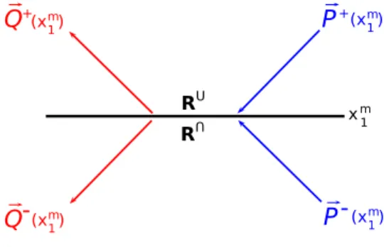
When the waveĄeld encounters a sharp velocity contrast, a part of the energy will scatter and a part will be transmitted. The incident waveĄeld at depth level 𝑥n
1 can be
written as:
⃗ 𝑄⊗(
𝑥n1) = R∪(
𝑥n1)𝑃⃗+(𝑥n1) +T∩(
𝑥n1)𝑃⃗⊗(
𝑥n1), (3.6a)
⃗ 𝑄+(𝑥n
1) = T
∪(
𝑥n
1)𝑃⃗+(𝑥n1) +R
∩(
𝑥n
1)𝑃⃗
⊗(
𝑥n
1), (3.6b)
where 𝑃⊗(
𝑥n
1) and 𝑃+(𝑥n1) are the upgoing and downgoing waveĄelds arriving at level
𝑥n
1. 𝑄
⊗(
𝑥n
1) and 𝑄+(𝑥n1) are the upgoing and downgoing waveĄelds leaving level 𝑥n1. The
operators R∪ and
R∩ are the reĆectivity coefficients acting on incident waves from above and from below respectively (see Figure 3.1). The operators T∪ and
T∩ are the analogous transmission operators. In acoustic approximation, the transmission coefficients are related by
R∪
=⊗R∩
=R (3.7a)
T∪ =I+R (3.7b)
T∩ =
I⊗R. (3.7c)
Figure 3.1 – Schematic representation of incoming and outgoing wavefields acting for each grid-point of depth level𝑥m1 .
Chapter 3. JOINT MIGRATION INVERSION 43
Then using equations 3.7 in 3.6, we Ąnd
⃗ 𝑄⊗(
𝑥n
1) = 𝑃⃗
⊗(
𝑥n
1) +Ó ⃗𝑃(𝑥n1) (3.8a)
⃗
𝑄+(𝑥n1) = 𝑃⃗+(𝑥n1) +Ó ⃗𝑃(𝑥n1), (3.8b)
where Ó ⃗𝑃 =R(︁𝑃⃗+⊗𝑃⃗⊗)︁ is the scattered waveĄeld.
Full WaveĄeld Modeling consists of recursive downgoing and upgoing extrapolation. The source waveĄeld𝑆⃗(𝑥0
1) is previously known, and the Ąelds outside the grid is assumed
to be zero. Schematically the recursive process is:
1. Modeling the downgoing waveĄeld (𝑚= 0,1,2, ..., 𝑀 ⊗1)
∙ At the surface, 𝑥0
1, add the source and the scattered waveĄelds:
⃗ 𝑄+(𝑥0
1) = 𝑃⃗+(𝑥01) +Ó ⃗𝑃(𝑥01) +𝑆⃗(𝑥01), (3.9)
for 𝑚̸= 0 add only the scattering:
⃗ 𝑄+(𝑥m
1 ) =𝑃⃗+(𝑥m1 ) +Ó ⃗𝑃(𝑥m1 ). (3.10)
∙ Then extrapolate the waveĄeld with downgoing extrapolation operator W+:
⃗
𝑃+(𝑥m+1
1 ) =W+(𝑥m1+1, 𝑥1m)𝑄⃗+(𝑥m1 ). (3.11)
2. Modeling the upgoing waveĄeld (𝑚=𝑀, 𝑀⊗1, 𝑀 ⊗2, ...,1)
∙ Add the scattered Ąeld:
⃗ 𝑄⊗
(𝑥m
1 ) =𝑃⃗
⊗ (𝑥m
1 ) +Ó ⃗𝑃(𝑥m1 ). (3.12)
∙ Extrapolate the waveĄeld with the upgoing extrapolation operator W⊗:
⃗
𝑃⊗(𝑥m1⊗1) =W
⊗
(𝑥m1⊗1, 𝑥m1 )𝑄⃗
⊗
(𝑥m1 ). (3.13)
When each round trip (downgoing extrapolation followed by upgoing extrapolation) is complete, it adds one order of two-way scattering. It is equivalent to the evaluation of the Neumann series. In the Ąrst round trip, 𝑃⃗+(𝑥m
1 ) and 𝑃⃗
⊗(
𝑥m
1 ) are assumed as zero
waveĄelds for every depth level 𝑥m
1 . Then we can summarize this process, according to
equations 3.11 and 3.13, as:
⃗
𝑃+(𝑥m1 ) = W+(𝑥1m, 𝑥01)𝑆⃗(𝑥01) +
m⊗1
∑︁
n=0
Chapter 3. JOINT MIGRATION INVERSION 44
⃗ 𝑃⊗(
𝑥m
1 ) =
M
∑︁
n=m+1
W⊗(
𝑥m
1 , 𝑥n1)Ó ⃗𝑃(𝑥n1), (3.14b)
where 𝑀 is the total samples in depth and
W+(𝑥m
1 , 𝑥n1) =
m
∏︁
k=n+1
W+(𝑥k
1, 𝑥k
⊗1
1 ), (3.15a)
W⊗ (𝑥m
1 , 𝑥n1) =
m
∏︁
k=n⊗1
W⊗ (𝑥k
1, 𝑥k1+1). (3.15b)
The user selects how many round trips will be evaluated.
3.2
Velocity perturbations
In JMI the phase of the waveĄeld only depends on the velocity model, which is related to the extrapolation operator W. JMI applies perturbation theory to the
extrapolation operator to extract information on the velocity perturbation, which will be used in a gradient descent scheme to minimize the difference between the modeled and recorded data in the least-squares sense. The algorithm is written in terms of the contrast parameter Õ(𝑥1, 𝑥2), deĄned as:
Õ(𝑥1, 𝑥2) = 1⊗
𝑐2
0(𝑥1, 𝑥2)
𝑐2(𝑥 1, 𝑥2)
, (3.16)
where 𝑐0(𝑥1, 𝑥2) is the background velocity and 𝑐(𝑥1, 𝑥2) the current velocity model. A
perturbation in the upgoing extrapolation operator is
ΔW⊗ (𝑥m
1 , 𝑥n1) =W
⊗ (𝑥m
1 , 𝑥n1)⊗W
⊗
0(𝑥m1 , 𝑥n1), (3.17)
where W⊗
0 is the background upgoing extrapolation operator. According equation 3.4 the
columns of Δ𝑊⊗ can be expressed as:
Δ𝑊⃗ ⊗ j (𝑥
m
1 , 𝑥n1) = ℱ
⊗1
x2
[︁
(𝑒⊗ikx1∆x1 ⊗𝑒⊗ik0∆x1)𝑒⊗ikx2x
j
2
]︁
, (3.18)
where 𝑘x1 =
√︁
𝑘2
0(1⊗Õ)⊗𝑘2x2 with 𝑘0 = c0ω. Equation 3.18 is the approximation of the
derivative in Õ, so that
Δ𝑊⃗ ⊗ j (𝑥
m
1 , 𝑥n1)≡
𝜕 ⃗𝑊⊗
𝜕Õ ⧹︃ ⧹︃ ⧹︃ ⧹︃ ⧹︃ ⧹︃ζ =ζ0
ΔÕ(𝑥n
1, 𝑥
j
2)≡𝐺⃗
⊗
0j(𝑥 m
1 , 𝑥n1)ΔÕ(𝑥n1, 𝑥
j
2), (3.19)
with
⃗ 𝐺⊗
0j(𝑥 m
1 , 𝑥
n
1) = ℱ
⊗1
x2
[︃
𝑖Δ𝑧
2
𝑘2 0
𝑘x1
𝑒⊗ikx1∆x1𝑒⊗ikx2x
j
2
⟨
ζ=ζ0
Chapter 3. JOINT MIGRATION INVERSION 45
Õ0 = 0 and ΔÕ =Õ. For 𝑘x1 = 0 (i.e at 90◇ propagation angle), expression 3.20 becomes unstable. To stabilize the division, a stabilization parameter 𝜀 can be used in 3.20:
⃗ 𝐺⊗0j(𝑥
m
1 , 𝑥
n
1) =ℱ
⊗1 x2
[︃
𝑖Δ𝑧
2 𝑘20
𝑘* x1
𝑘*
x1𝑘x1 +𝜀
𝑒⊗ikx1∆z𝑒⊗ikx2x
j
2
⟨
ζ=ζ0
, (3.21)
where* denotes the complex conjugation. The complete matrix ΔW⊗
0(𝑥m1 , 𝑥n1) is written
as:
ΔW⊗
0(𝑥m1 , 𝑥n1) =G
⊗
0(𝑥m1 , 𝑥n1)ζ(𝑥n1), (3.22)
whereζ(𝑥n
1) is a diagonal matrix with𝑑𝑖𝑎𝑔[ζ(𝑥1n)] =⃗Õ(𝑥n1) being the velocity perturbations
at depth level 𝑥n
1. Individually, all velocity perturbations are carried to the surface by
G⊗0(𝑥01, 𝑥n1) = W⊗0(𝑥01, 𝑥1n⊗1)G⊗0(𝑥1n⊗1, 𝑥n1), (3.23)
and these effects are measured as a scattered waveĄeld
Δ𝑃⃗⊗ ζ (𝑥01) =
N
∑︁
n=1
G⊗
0(𝑥01, 𝑥
n
1)ζ(𝑥
n
1)𝑄⃗
⊗(
𝑥n1). (3.24)
3.3
Reflectivity perturbations
This work didnŠt take account the angle-dependency of reĆectivity. The reĆectivity operators are diagonal matrix, where 𝑑𝑖𝑎𝑔[R∪
0(𝑥n1)] =⃗𝑟(𝑥n1) are the reĆectivities at depth
level 𝑥n
1. The effect of perturbation is derived directly from equation 3.6a, where only
the reĆected amplitude, R∪
𝑃+(𝑥n
1), matters for the receivers detection at the surface, so
that the scattered waveĄeld at the reĆectivity perturbation can be written, in analogy to equation 3.24, as
ΔP⊗
∆r(𝑥
0
1) =
N
∑︁
n=1
W⊗ (𝑥01, 𝑥n
1)ΔR(𝑥n1)𝑃⃗+(𝑥n1). (3.25)
3.4
Inversion
JMI estimates the velocity and reĆectivity models by minimizing the difference between the observed and modeled data as indicated by the objective function
𝐽 =
ω2
∑︁
ω1
♣♣P⊗
obs(𝑥01)⊗P
⊗
mod(𝑥01)♣♣2 =
ω2
∑︁
ω1
♣♣ΔP⊗(𝑥01)♣♣2, (3.26)
where [æ1, æ2] is the frequency bandwidth of modeling and the matrixP(𝑥01) is the collection
of all shot measurements 𝑃⃗(𝑥0
1). According to equations 3.24 and 3.25, the gradients for
velocity and reĆectivity, calculated at depth level 𝑥n
1, are:
∇⃗Õ(𝑥n1) = 𝑑𝑖𝑎𝑔 (︃ω2
∑︁
ω1
[︁
G⊗(𝑥n1, 𝑥01) ]︁H
ΔP(𝑥01) [︁
Q⊗(𝑥n1) ]︁H)︃
Chapter 3. JOINT MIGRATION INVERSION 46
∇⃗𝑟(𝑥n
1) = 𝑑𝑖𝑎𝑔
(︃ω2 ∑︁
ω1
[︁
W⊗(
𝑥n
1, 𝑥01) ]︁H
ΔP(𝑥01)[︁P+(𝑥n
1) ]︁H)︃
, (3.27b)
where the operatorsWandGare evaluated for the current velocity and reĆectivity models.
The waveĄeld perturbation predicted by these gradients are:
Δ𝑃⃗⊗
∇r(𝑥01) =
N
∑︁
n=1
W⊗(𝑥01, 𝑥n1)∇R(𝑥n1)𝑃⃗+(𝑥n1) (3.28a)
Δ𝑃⃗⊗
∇ζ(𝑥01) =
N
∑︁
n=1
G⊗
0(𝑥01, 𝑥n1)∇ζ(𝑥n1)𝑄⃗
⊗(
𝑥n
1), (3.28b)
where 𝑑𝑖𝑎𝑔[∇R(𝑥n
1)] = ∇⃗𝑟(𝑥n1) and 𝑑𝑖𝑎𝑔[∇ζ(𝑥n1)] = ⃗Õ(𝑥n1). Finally the update formulas
for reĆectivity and velocity are:
𝑟new(𝑥1, 𝑥2) =𝑟old(𝑥1, 𝑥2) +Ðr∇𝑟(𝑥1, 𝑥2) (3.29a)
𝑐new(𝑥1, 𝑥2) =
𝑐old(𝑥1, 𝑥2) √︁
1⊗Ðζ∇Õ(𝑥1, 𝑥2)
, (3.29b)
with
Ðζ = arg min αζ
(︃ω2 ∑︁
ω1
♣♣ΔP⊗(𝑥01)⊗ÐζΔP⊗∇ζ(𝑥01)♣♣2 )︃
(3.30a)
Ðr = arg min αr
(︃ω2 ∑︁
ω1
♣♣ΔP⊗(
𝑥01)⊗ÐrΔP⊗
∇r(𝑥01)♣♣2 )︃
. (3.30b)
Schematically a single iteration of JMI is summarized as follows:
1. Update the reĆectivity for each depth level:
∙ Update the waveĄelds P+(𝑥m
1 ) andP
⊗(
𝑥m
1 ) according the equations 3.14a and
3.14b for the most recent velocity and reĆectivity estimates.
∙ Calculate the reĆectivity gradient∇⃗𝑟(𝑥1, 𝑥2), equation 3.27b.
∙ Calculate the waveĄeld perturbation ΔP⊗∇r(𝑥01), equation 3.28b, and Ðr,
equa-tion 3.30b
∙ Update the reĆectivity, equation 3.29a
2. Update the velocity for each depth level:
∙ Update the waveĄelds P+(𝑥m
1 ) andP
⊗(
𝑥m
1 ) according the equations 3.14a and
3.14b for the most recent velocity and reĆectivity estimated (one round trip).
∙ Calculate the velocity gradient ∇⃗Õ(𝑥1, 𝑥2), equation 3.27a.
∙ Calculate the waveĄeld perturbation ΔP⊗
∇ζ(𝑥01), equation 3.28a, and Ðζ,
equa-tion 3.30a
Chapter 3. JOINT MIGRATION INVERSION 47
3. Repeat 1 and 2 steps until the objective function𝐽 gets minimum or if the maximum
iterations has been achieved.
JMI needs to specify the frequency range [æ1, æ2]. Normally the strategy is to
choose a low frequency for æ1 and to increase the bandwidth as optimization proceeds.