The Douglas-Peucker Algorithm: Sufficiency Conditions for
Non-Self-Intersections
1Shin-Ting Wu & Adler C. G. da Silva & Mercedes R. G. Márquez
Universidade Estadual de Campinas (UNICAMP)
Faculdade de Engenharia Elétrica e Computação (FEEC)
Departamento de Engenharia de Computação e Automação Industrial (DCA) {ting,acardoso,meche}@dca.fee.unicamp.br
December 12, 2006
ABSTRACT
The classic Douglas-Peucker line-simplification algorithm is recognized as the one that delivers the best perceptual representations of the original lines. It may, however, produce simplified polyline that is not topologically equivalent to the original one consisting of all vertex samples. On the basis of properties of the polyline hulls, Saalfeld devised a simple rule for detecting topological inconsistencies and proposed to solve them by carrying additional refinements. In this paper, we present an alternative form for the classic Douglas-Peucker to produce a simplified polyline which is homeomorphic to the original one. Our modified Douglas-Peucker algorithm is based on two propositions: (1) when an original polyline is star-shaped, its simplification from the Douglas-Peucker procedure cannot self-intersect; and (2) for any polyline, two of its star-shaped sub-polylines may only intersect if there is a vertex of one simplified sub-polyline inside the other’s corresponding region.
Keywords: Topological Consistency; Line Simplification; Douglas-Peucker Algorithm; GIS.
1 Introduction
Often the geometric resolution of a polyline is much higher than the resolution supported by the application, such as visualization of geographic map boundaries or visualization of curves approximated by sampling a parametric curve at regular small intervals in a raster display. For the sake of efficiency, we search for algorithms that can extract essential features from detailed data of the original polyline and represent them on a simple one having fewer vertices, sufficient for the specified resolution. Many of them have been pursued by the researchers in different contexts [5, 6, 8, 11, 12, 14].
farther away than that maximum distance is accepted as part of the new simplified polyline, and it becomes the new initial vertex for further simplification [10].
From detailed study of mathematical similarity and discrepancy measures, the Douglas-Peucker algorithm is pointed out as the most visually effective line simplification algorithm [1, 7]. Whereas vertex reduction uses closeness of vertices as a rejection criterion, the Douglas-Peucker algorithm uses the closeness of a vertex to the simplified polyline. It is a recursive procedure that starts with a line segment whose extreme vertices coincide with the extreme vertices v
1 and vn of the polyline given as a
list of n vertices in sorted order. Each segment v
kvj is split at the farthest vertex vi to it, where k < i <
j, until the distance between the sequence of vertices v
k⋅⋅⋅vi and vkvi and the distance between the
sequence of vertices v
i⋅⋅⋅vj and vivj are less than a fixed tolerance.
Saalfeld performed a thorough analysis of the Douglas-Peucker algorithm and listed in [9] a set of its key properties. Besides, on the basis of the hull property of the simplified polyline obtained from the Douglas-Peucker algorithm, he proposed, with proof, to use a point-on-convex hull test and the sidedness concept for detecting possible topological conflicts. He used the dynamic convex hull algorithm presented by Hershberger and Snoeyink [3] to efficiently maintain and access the current convex hull at each refinement stage.
This paper presents yet three contributions to deal with the self-intersection problem in the Douglas-Peucker algorithm. The first is a proof for the fact that the simplification of a star-shaped polyline by the Douglas-Peucker method will never result in a self-intersecting polyline. The second is a procedure for trivially discarding segments of a simplified polyline that do not intersect. And finally, on the basis of the first and the second contributions we propose a non-self-intersecting Douglas-Peucker algorithm for any polyline.
In Section 2, the Douglas-Peucker algorithm is briefly described for completeness. The proof of the sufficiency conditions for non-self-intersections is presented in Section 3. Section 4 gives a strategy for eliminating possible conflicts between simplified sub-polylines. In Section 5, we describe our polyline simplification algorithm that integrates these two properties into the classic Douglas-Peucker to ensure topological equivalence between the original and the simplified polylines for any specified tolerance. Section 6 details a complexity analysis of the algorithm. Afterwards, some results are shown in Section 7. Finally, in Section 8, our future research directions are presented.
2 The Douglas-Peucker Algorithm
Besides its good visual results, the Douglas-Peucker algorithm is very simple to program and works for any dimension, once it only relies on the distance between points and lines. Several implementations are available at sites of the Internet [2, 10]. Its basic rule is that the approximation must contain (a subset of) the original data points and all the original data points must lie within a certain predefined distance to the approximation.
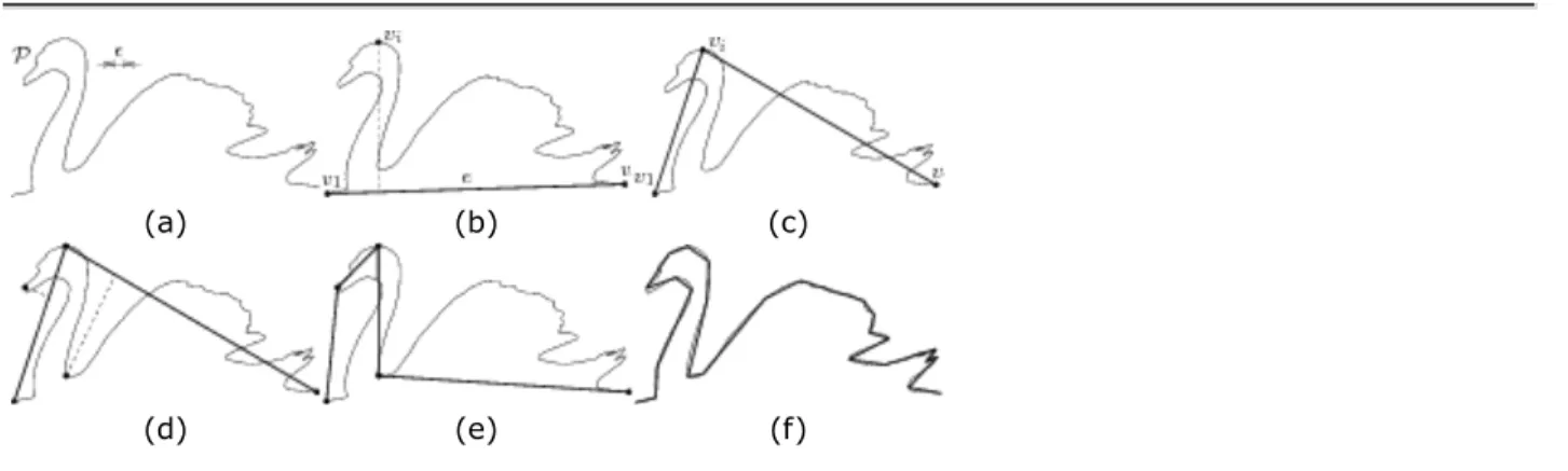
Given a polyline P and a tolerance ε as depicted in Figure 1.a. The Douglas-Peucker algorithm has a hierarchical structure starting with the single line segment e joining the first v
1 and last vn vertices of
the original polyline (Figure 1.b). Then the remaining vertices are tested for closeness to its approximating segment. If there are vertices farther than some specified tolerance away from the segment, then the vertex v
new approximation for the original polyline (Figure 1.c). Recursively this process continues for each approximating line segment (Figures 1.d,e) until all vertices of the original polyline satisfy the closeness condition (Figure 1.f).
(a) (b) (c)
(d) (e) (f)
Figure 1: The basic Douglas-Peucker algorithm.
This algorithm has O(mn) worst-case time complexity and O(nlog n) expected time, where n is the number of input vertices and m is the number of the vertices of the simplified polyline. This is an output dependent algorithm and it will be very fast when m is small, that is when the approximation is coarser. On the other hand, if the tolerance has a larger value, then the simplified polyline may intersect itself. Figure 2 illustrates a case for which three splittings on the initial segment e were sufficient for satisfying the tolerance condition, but could not avoid self-intersection. The trivial solution is to reduce the value of the tolerance, which may lead to a unnecessarily finer approximation.
Figure 2: Self-intersection.
An alternative for solving this problem is to keep on applying the Douglas-Peucker procedure only on the part of the simplified polyline that presents topological conflicts. More specifically, Saalfeld [9] proposed the following procedure for detecting and solving topological conflicts in relation to each segment e
ij approximating a sub-polyline Pij which is, in its turn, a subset of the original polyline P:
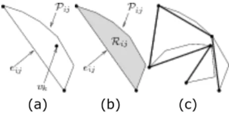
Identify all vertices v
k (Figure 3.a), where k < i or k > j, of the simplified polyline that lie in the
region R
ij bordered by the sequence of vertices belonging to the sub-polyline Pij and the
segment e
ij (Figure 3.b).
1.
Recursively split e
ij until every vertex, such as vk, is out the region limited by the simplified and
(a) (b) (c)
Figure 3: Further splitting until v
k becomes out.
3 Sufficiency for Non-Self-Intersections
Before demonstrating the sufficiency conditions for a simplified polyline generated by the Douglas-Peucker algorithm to be non-self-intersecting, we introduce some definitions.
Definition 3.1 The convex hull H of a set of points S is the smallest set containing S that satisfies the following convexity property: for any pair of points p,q ∈ H the line segment pq is completely contained in H.
Definition 3.2 Let P be an open polyline as a list of n vertices v
1,v2,…,vn in sorted order, and r a point on
the segment v
1vn, excluding the extreme vertices. We say that P is star-shaped with respect to r, if, for
any point p ∈P, the ray
-→rp intersects P only at p (Figure 4).
Figure 4: A star-shaped polyline.
Observe that the line segments rv
i, where i ∈{1,2,…,n}, build with (n - 1) segments of a star-shaped
polyline a set of edge-adjacent, but non-overlapping, triangles. Based on this, we are able to present the following proposition.
Proposition 3.1 Given a star-shaped polyline P as a list of n vertices v
1,v2,…,vn in sorted order, its
simplification from the Douglas-Peucker procedure cannot self-intersect.
Proof: We prove the proposition by induction on m output vertices in the simplified polyline. When m = 3, the simplified polyline consists of the two extreme points, v
1 and vn, and a vertex vk, where 1 < k
< n, farthest from the line segment v
self-intersect.
When m > 3 and assume that the proposition is true for all values less than m. Let v
b be the newly
inserted vertex and is farthest from the line segment v
avc, where a < b < c; the line segments vavb
and v
bvc only intersect at vb and cannot intersect the simplified sub-polylines v1⋅⋅⋅va and vc⋅⋅⋅vn,
because such an intersection implies that the triangle rv
avb and/or rvcvb overlap another triangle rvkvl,
where k⁄=l and k,l = 1,…,a,c,…,n, contradicting the star-shapeness property. Hence, the simplified polyline consisting of m vertices cannot self-intersect.
4 Sufficiency for Non-Intersection between Sub-Polylines
The sidedness of a vertex with respect to the simplified and original polylines may not be preserved by the Douglas-Peucker algorithm. In his work, Saalfeld concluded that topological conflicts always occur when vertices of the simplified polyline change their sidedness. He also suggested to use the data structure presented by Hershberger and Snoeyink [3] for reducing the search space of potential conflicts at each refinement recursion as well.
We showed in Section 3 that, by applying the Douglas-Peucker algorithm on a star-shaped polyline, the simplified polyline never self-intersects. So a possible approach for simplifying a non-star-shaped polyline would be to first decompose it into star-shaped sub-polylines and then apply the Douglas-Peucker algorithm on each sub-polyline. Nevertheless, this approach cannot ensure that non-self-intersecting piecewise simplified sub-polylines do not cross. In this section, we present a sufficient condition for non-intersections between two sub-polylines. Before this, let us introduce the following definition, which is useful to distinguish the two sides of a polyline on a plane.
Definition 4.1 A polyline P = {v
1,v2,…,vn} is orientable if there exists a simply-connected region R
whose boundary is the closed sequence v
1,v2,…,vn,v1. If the sorted order of the vertices is in the
clockwise sense along the boundary of R, P is said to be clockwise oriented with respect to R (Figure 5.a); otherwise, it is counter-clockwise oriented (Figure 5.b). The region R is called polyline region.
(a) Clockwise oriented(b) Counter-clockwise oriented
Figure 5: Orientable polylines.
orientable polyline. This is because that the union of a set of edge-adjacent and non-overlapping triangles with a common vertex is a simply-connected region and a star-shaped polyline is the boundary of this set of triangles.
Proposition 4.1 Let P and Q be two orientable polylines that have at most some points in common. Let R and S be the respective polyline regions that have only these points in common. Let P
s and Qs be the
corresponding simplifications of P and Q. If P
s∈ R, where Qs∈ S, then Ps and Qs have at most those
points in common.
Proof: If P
s and Qs have other points in common, then R and S must have more common points,
because P
s∈R and Qs∈S. This contradicts the supposition. Hence, Ps and Qs can share at most the
common points of P and Q.
Proposition 4.1 tells us that if a polyline is partitioned into a set of orientable sub-polylines, such that their regions have at most the extreme or the boundary points in common, then we may restrict the search space for potential topological conflicts to the simplified sub-polylines that do not lie entirely in the region of their corresponding original sub-polylines. Figure 6 presents two cases: (a) P
s∈R, Qs∈S;
and (b) P
s∈⁄R, Qs∈⁄S. Conflicts may only occur in the second case.
(a) (b)
Figure 6: Potential topological conflicts.
Let us introduce one more definition before presenting a practical corollary.
Definition 4.2 Two orientable polylines are called separable, if their polyline regions have at most the extreme or boundary points in common (Figure 7).
(a) Separable polylines (b) Non-separable polylines
Figure 7: Separability of two polylines.
Proof: If the simplified polylines intersect at their interior points, the corresponding polyline regions must intersect at some interior points, which violates the definition of separable polylines.
5 A Non-Self-Intersecting Douglas-Peucker Algorithm
Based on the properties presented in Sections 3 and 4, we present a modified Douglas-Peucker simplification method that may avoid self-intersections along the recursive refinements of a polyline P with n input vertices v
1,v2,…,vn and that can detect the potential topological conflicts with a simple
sidedness test. The algorithm comprises three steps:
Partition P into a set C of separable star-shaped sub-polylines. 1.
Apply the Douglas-Peucker algorithm for every sub-polyline C
i∈C.
2.
Beside topological conflicts between the sub-polylines. 3.
5.1 Partition into separable star-shaped polylines
According to Corollary 4.1, the simplified polylines of two separable star-shaped polylines cannot intersect except at the boundary vertices of their polyline regions, if they lie entirely in the
corresponding polyline regions. Moreover, Proposition 3.1 tells us that the simplified polyline of any star-shaped polyline cannot self-intersect. This motivates us to decompose an input polyline P into a set of separable star-shaped polylines before carrying out the Douglas-Peucker procedure at each one. We devised a two-step procedure for partitioning any open polyline P. In the first step, P is partitioned into a set of separable sub-polylines; and, in the second step, we apply a visibility algorithm to decompose each orientable sub-polyline into non-overlapping star-shaped pieces.
5.1.1 First Step
The support line of the vector
--→ v1vn divides P in two parts: its left side and its right side (Figure 8.a). We determine the intersection points u
1,u2,…,ur. Then, they are sorted along the direction of the vector
--→ v1vn , and P is split at them into subsequences of vertices, as shown in Figure 8.b. For instance,
u
1⋅⋅⋅u2 and u5⋅⋅⋅u6 are two distinct subsequences of P.
(a) (b) (c) (d)
Figure 8: Partition into a set of separable sub-polylines.
We can determine all regions, R
1,R2…Rl, by simply tracing along the support line twice: one turn in the
-v-1→vn and another turn in the direction
-v-n→v1 . This is because the side of a region alternates between in (I) and out (O) at each intersection
point, as depicted in Figure 8.c. Hence, we may link the intersection points in sorted order to build the separable polylines on the left side, in the case P
2, and, analogously on the right side, to obtain P1 and
P
3 (Figure 8.d).
5.1.2 Second Step
To determine a star-shaped sub-polyline of a polyline with respect to a point r is similar to the classic problem of computing a visibility polygon from r. Our implementation is based on the Hipke’s linear time algorithm [4]. For decomposing a polyline with n vertices P = {v
1,v2,…,vn} into a set of star-shaped
polylines, we apply the algorithm on P to obtain a visibility polygon V; then we replace P by P-V and apply the algorithm recursively until no vertex remains.
For the sake of completeness, an outline of Hipke’s algorithm is given in this section. The algorithm scans the n vertices of the polyline P in sorted order and chooses the visible ones on the basis of the tracking sense at each vertex and on the mode of operation, which depends only on the current and previous tracking senses.
According to the signal of the turn angle φ, that is the angle between the segments rv
i-1 and rvi, two
senses are distinguished: forward or positive (Figure 9.a), and backward or negative (Figure 9.b).
(a) Forward tracking(b) Backward tracking
Figure 9: Tracking senses.
Backward trackings are further subdivided into inward (the segment v
i-1vi lies between the
segment v
i-2vi-1 and the point r, as shows Figure 10.a) and outward (the segment vi-2vi-1 lies between
the segment v
i-1vi and the point r, as illustrates Figure 10.b).
(a) Inward tracking(b) Outward tracking
Three modes are distinguished: normal, skip and curl. In the normal mode, the current vertex is inside the scanned star-shaped polyline V. In both skip and curl modes, the current vertex is not visible and the algorithm waits to come back into the area of V. Switching from the normal mode to one of these two modes depends on the way how the tracking tends to progress when it passes from a visible to a non-visible vertex: when it seems to advance spirally, as shown in Figure 11.a, the vertices will be further scanned in the curl mode; otherwise, we enter the skip mode (Figure 11.b).
(a) Curl mode(b) Skip mode
Figure 11: Modes for handling non-visible vertices.
For distinguishing correctly the visible from non-visible vertices, the algorithm demands a stack of skip segments that grows, whenever the skip mode is activated, or shrinks, if any skip segment becomes obscured. Each skip segment is represented by its first point s and its end point q. The points at which the polyline starts curling are also represented as curl points.
The procedure starts at v
i = v2 in the normal operation mode. It also considers that the previous
tracking sense was forward. The vertices are scanned sequentially from i = 2 to n. We may be in one of the three modes of operation at each vertex v
i:
normal mode: if the tracking sense is
forward: if the previous sense was in-backward and rv
i intersects the support line
of v
i-2vi-1, set vi-1 as the curl point, skip vi and switch to the curl mode; otherwise, vi is
inserted in the output list V. out-backward: pile v
i-1 as the initial point of a skip segment, skip vi, and switch to the skip
mode.
in-backward: if the segment v
i-1vi crosses any skip segment, remove from the output
list V all vertices v
j, with j < i, until vk (the first visible vertex after the skip segment), pop
out all skip segments with end points v
l, where l > k, and switch to the skip mode;
otherwise, remove from the output list V all vertices v
j, with j < i, until a segment in V
intersects the ray beginning at r and passing through v
i, and insert vertex vi in V.
1.
skip mode: if the segment v
i-1vi intersects the ray beginning at r and passing through s (the first
point of the current skip segment), then determine the intersection point q, set it as the end point of the current skip segment, add v
i in the output list V, and switch to the normal mode;
otherwise, skip vertex v
i and keep on the skip mode.
2.
curl mode: if the segment v
i-1vi intersects the ray beginning at r and passing through c (the curl
point), then add v
i in the output list V and switch to the normal mode; otherwise, skip vi, and
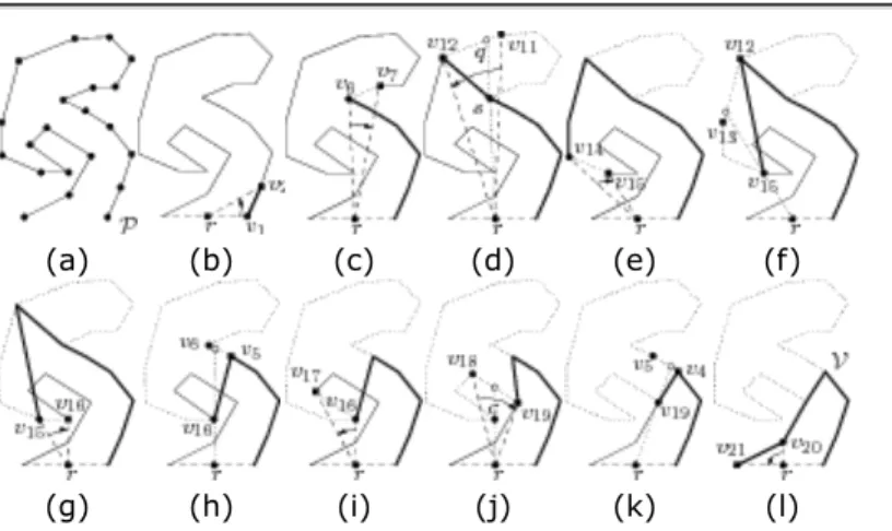
Figure 12 illustrates an application of this procedure to the polyline P in Figure 12.a. In the figure, the current vertex is highlighted with a black square, the intersection points are indicated by the white circles, and the current tracking sense is pointed out by a curved arrow.
The algorithm starts in the normal mode at the vertex v
2. The (current) tracking sense from v1 to v2 is
forward (Figure 12.b). It continues moving forward, until it finds the out-backward tracking from v
6
to v
7 (Figure 12.c). It then sets v6 as the current skip point s and enters the skip mode. It begins
skipping vertices, until it reaches the end point q – the intersection between the ray rs and the segment v
11v12 – of the current skip segment (Figure 12.d). In consequence, it returns to the normal mode.
The algorithm moves further forward until the in-backward tracking is detected at v
15 (Figure 12.e). It
begins removing vertices previously inserted in the output list, until it finds the intersection between the segment v
12v13 and the ray rv15 (Figure 12.f). As the movement from v15 to v16 is in-backward
(Figure 12.g), it pops out the skip segment sq and discards all vertices from the output list, until it finds an intersection between the ray rv
16 and the segment v5v6 (Figure 12.h). At v17 the spiral movement is
identified, then v
16 is assigned as the curl point c and the procedure enters the curl mode (Figure 12.i).
In consequence, all subsequent vertices are ignored, until the intersection between rc and v
18v19 is
reached. The normal mode is then restored.
The procedure reevaluates the state of the output list with regard to v
19. As the tracking from v18
to v
19 is in-backward, it have to remove all the vertices from the output list till the intersection
between rv
19 and v4v5 (Figure 12.k). Further forward progress until the end vertex v21 results in the
star-shaped polyline V (Figure 12.l).
(a) (b) (c) (d) (e) (f)
(g) (h) (i) (j) (k) (l)
Figure 12: Determination of a star-shaped polyline.
5.2 Beside Topological Conflicts
If we consider that each star-shaped polyline is clockwise oriented, this sidedness test is equivalent to the condition that there is a sample v
j between vi and vk, where i < j < k, for which the third coordinate
(z-coordinate) of the cross product (v
kvj× vjvi) is equal to or greater than zero
z(vkvj × vjvi) ≥ 0. (1) This allows us to reduce the search space for the topological conflicts and to carry out the intersection test only between the star-shaped polylines that violate Eq. 1.
Figure 13 illustrates the proposed procedure. Figure 13.a presents three segments (d
1, d2 and d3) that
do not lie in the corresponding polyline region. There is only a vertex that violates Eq. 1 with regard to d
1. Hence, d1 is further refined until Eq. 1 is satisfied (Figure 13.b).
(a) (b)
Figure 13: Besiding topological conflicts.
6 Complexity Analysis
There is a variety of ways to implement our algorithm, since a number of algorithms is available for solving each subproblem. In this section we present a time complexity analysis of our algorithm as we implemented it.
For partitioning an input polyline with n vertices into a set of separable polylines, we first find all points that intersect the support line. This is performed in O(n) time. After then, we sort r intersection points in O(r log r) time. We finally join the pieces to build a set of separable simple polylines with O(r) time. Therefore, the worst-case time complexity of this step is O(n + r log r + r), or simply O(n + r log r). The worst case for partitioning any polyline with n vertices into a set of l star-shaped ones occurs when it is already separable, that is r = 1. Since the algorithm for determining a star-shaped polyline we used is linear, the worst-case complexity of the whole partitioning is O(ln). However, the number of
star-shaped polylines l is always less than the number of output vertices m. So, we can upperbound its complexity to O(mn).
We know as well that the algorithm for finding the farthest vertex of a sequence, used exhaustively in Douglas-Peucker simplification, is linear. Then, the Douglas-Peucker algorithm runs for each
For handling the topological conflicts between the star-shaped polylines, we have to verify every external segment of a simplified polyline against all segments of the others. In the worst case, this check is performed in O(m2) time.
Finally, for regrouping the separable polylines, built in preprocessing, into one sequence as the output, we have just to pass through every output vertex sequentially, what takes O(m) time.
For computing the whole complexity, we add together the worst-case complexity of each step, that results in
O(n+ rlogr +mn + m2 +m) (2) Since the number of input vertices n is always greater than or equal to the number of output
vertices m, the three last terms of the sum in Eq. 2 fulfills the inequality 2 mn +m + m ≤ mn + mn + mn.
In addition, once the preceding vertex and the subsequent vertex of the intersection points are always included in the simplified polyline, the number of output vertices m is greater than the number of intersection points r. Thus, for the first two terms of the sum in Eq. 2, we have
n+ r logr < n+ m logm < n + mn ≤ mn + mn.
Summarizing, the worst-case complexity of our algorithm is O(mn), which is equivalent to the time complexity of the original Douglas-Peucker algorithm we used in our implementation.
7 Results
To evaluate the algorithm we implemented, we present in this section some results we obtained on the simplification of the outlines of the continents from the atlas data available at [13]. Comparisons with the results from the original Douglas-Peucker algorithm [1] are also provided.
Figure 14.a illustrates a Europe’s outline with 53,626 vertices. Its Douglas-Peucker simplification with a tolerance of 4.0 contains 18 vertices and two self-intersections, which are encircled by the dashed line in Figure 14.b. The reduced outline from our algorithm (Figure 14.c) has no self-intersections, although it possesses much more vertices (46), 22 of which were inserted during the partition into separable polylines and 24 were added for splitting them into star-shaped ones. It is worth noting that in
Figure 14.c the shape of Scandinavian Peninsula is much more distorted than in Figure 14.b. It is due to the partition of the original outline into star-shaped polylines before performing the Douglas-Peucker algorithm.
(a) (b) (c)
with tolerance of 4.0.
Figure 15.a shows an Asia’s outline with 87,337 vertices. Figures 15.b and 15.c are respectively the simplified outlines, with tolerance of 8.6, from the Douglas-Peucker and our algorithm. Because of high tolerance and wavy outline, the original Douglas-Peucker algorithm delivers self-intersections (encircled by the dashed line) in a very reduced outline, with only 13 vertices. As expected, the result of our algorithm is self-intersection free, at cost of more vertices (35) in the output: 15 of them were inserted while the original polyline was splitted into star-shaped sub-polylines.
(a)
(b) (c)
Figure 15: Comparison between Douglas-Peucker and our approach simplifications of Asia’s map with tolerance of 8.6.
Figures 16.a and 16.b present, respectively, the simplifications with tolerance of 0.3 of the North America’s outline from the Douglas-Peucker and our proposal. The number of vertices in the original outline is 105,499. The Douglas-Peucker algorithm reduces it to 993 vertices, but because of highly wavy borderline 54 self-intersections were resulted. Although our algorithm delivers much more
number of vertices in the output (1,717), it contains no self-intersections. Visually, the results are much alike.
(a) (b)
Figure 16: Simplifications of the North America’s outline with tolerance of 0.3.
closely laid in the position pointed in Figure 17.b. Figure 17.c shows our simplification with 27 vertices, where 16 vertices introduced in preprocessing are laid closely in the position indicated by the arrow in Figure 17.c. As expected, for avoiding self-intersections, low tolerance may lead to an excessive number of star-shaped sub-polylines in the protruding polyline.
(a) (b) (c)
Figure 17: Simplifications of the Oceania’s outline with tolerance of 4.2.
Figure 18.a illustrates an Africa’s outline with 28,653 vertices. Its Douglas-Peucker simplification, with tolerance of 4.5, contains 11 vertices, as depicted in Figure 18.b. Because its undulations are relatively larger with respect to the specified tolerance, the number of vertices in the output of our algorithm is almost the same: 19. Moreover, the reduced outlines in Figure 18.b and Figure 18.c are very similar.
(a) (b) (c)
Figure 18: Simplifications of the Africa’s outline with tolerance of 4.5.
Table 1 summarizes the results obtained with the use of the Douglas-Peucker algorithm and our algorithm. The column “Input” contains the number of input vertices. The simplification tolerance is given in the column “ε”. The output is recorded in the column “Output”. The number of occurrences of self-intersections is in the column “S-I”. We also show the number of inserted vertices in the
preprocessing (“Pre”) and during the partition into the star-shaped polylines and the elimination of topological conflicts (“Post”). Additionally, the processing time for each simplification is given in seconds in the column “t(s)”.
Data DP algorithm Our algorithm
Oceania 27,5774.2 9 01.010 27 16 111.390 Africa 28,6534.5 11 01.070 19 6 131.450 Europe 53,6264.0 18 21.990 46 22 242.690 Asia 87,3378.6 13 13.260 35 15 204.400 North America105,4990.3 993 544.170 1,7171031,6147.510
Table 1: Summary of maps simplification results.
Observe that our procedure has a simplification ratio comparable to the Douglas-Peucker procedure with the advantage that no self-intersection appears. We did not perform detailed measurements for analyzing the visual effect of our algorithm. However, the simplified polylines we obtained are fair from our subjective judgment, once most of extra vertices that our procedure introduced are in the portion of the simplified polyline that has a large variation in the curvature.
8 Concluding Remarks
In this paper, we present yet an improvement to the classic Douglas-Peucker line simplification
algorithm in terms of preventing self-intersections. We derive, with proof, two sufficient conditions. On the basis of these conditions, we also propose a way to integrate them into the Douglas-Peucker algorithm and to reduce the search space for the topological violations. The concept of polyline region was not only useful for trivially discarding star-shaped sub-polylines that cannot cause any topological conflicts, but also for controlling further local refinements as well.
Another contribution of our work is the decomposition of the problem into a set of sub-problems whose solutions are well-known. This facilitated the implementation of our algorithm and the validation of our idea. From the experiments we carried out, the results of our algorithm are similar to the ones
produced by the classic Douglas-Peucker algorithm, except in the vicinity of the connecting vertices of the star-shaped polylines.
Our algorithm tends to refine much more. The focus of this work is the robustness of simplification, and not the efficiency. Hence, we did not investigate its performance thoroughly. From a quick analysis, our implemented algorithm has, like the classic Douglas-Peucker algorithm, O(mn) worst-case time, where m is the number of output vertices, and n the number of input vertices. This performance is output dependent.
As further work, we may improve the performance of our algorithm by optimizing the decomposition of the input polyline into a set of separable polylines. It is also interesting to compare the performance of the optimized algorithm with the existing ones.
Acknowledgments
We would like to acknowledge the State of São Paulo Research Foundation (FAPESP, Grant No 00/10913-3) and the Coordination for the Improvement of Higher Education Personnel Foundation (CAPES) for financial support.
Notes
1
Based on "A non-self-intersection Douglas-Peucker Algorithm", by Wu, Shin-Ting and Márquez, Mercedes R. G. which appeared in Proceedings of Sibgrapi 2003. © 2004 IEEE.
References
1. D. Douglas and T. Peucker. Algorithms for the reduction of the number of points required for represent a digitzed line or its caricature. Canadian Cartographer, 10(2):112–122, 1973.
2. J. De Halleux. An C++ implementation of Douglas-Peucker line approximation algorithm, 2003.
http://www.codeproject.com/useritems/dphull.asp.
3. J. Hershberger and J. Snoeyink. Speeding up the Douglas-Peucker line simplification algorithm. In The 5th International Symposium on Spatial Data Handling, volume 1, pages 134–143, 1992. 4. C. A. Hipke. Computing visibility polygons with LEDA, 1996.
5. G. F. Jenks. Lines, computers and human frailties. In Annals of the Association of American Geographers, pages 1–10, 1981.
6. T. Lang. Rules for robot draughtsmen. Geographical Magazine, 22:50–51, 1969.
7. U. Ramer. An iterative procedure for the polygonal approximation of plane curves. Computer Graphics and Image Processing, 1:224–256, 1972.
8. K. Reumann and A. P. M. Witkam. Optimizing curve segmentation in computer graphics. In Proceedings of the International Computing Symposium, pages 467–472, 1974.
9. A. Saalfeld. Topologically consistent line simplification with the Douglas Peucker algorithm. Cartography and Geographic Information Science, 26(1):7–18, 1999.
10. Dan Sunday. Geometric algorithms. http://geometryalgorithms.com/Archive/algorithm_0205 /algorithm_0205.htm.
11. W. R. Tobler. An experiment in the computer generalization of map. Technical report, Office of Naval Research, Geography Branch, 1964.
12. M. Visvalingam and J. D. Whyatt. Line generalisation by repeated elimination of points. Cartographic Journal, 30(1):46–51, 1993.