M´ario Foganholi Fernandes
Universidade Federal de Minas Gerais
Instituto de Ciˆencias Exatas – Departamento de F´ısica
Phase retrieval algorithms
applied to the reconstruction of
photonic quantum states
M´ario Foganholi Fernandes
Advisor: Leonardo Teixeira Neves
Co-advisor: Miguel ´Angel Sol´ıs Prosser∗
∗Center for Optics and Photonics, Departamento de F´ısica,
Universidad de Concepci´on, Chile
practice is always to keep our be-ginner’s mind. In the bebe-ginner’s mind, there are many possibili-ties; in the expert’s mind there are few.
—Shunryu Suzuki-roshi
All life demands struggle. The very striving and hard work that we so constantly try to avoid is the major building block in the person we are today.
Acknowledgements
Eu gostaria de agradecer, primeiramente, ao meu orientador, Leonardo Neves, e ao meu co-orientador, Miguel Sol´ıs Prosser. Trabalhar com vocˆes tem sido incrivelmente enriquecedor, tanto pelo lado acadˆemico quanto pelo pessoal, pois vocˆes me ensinam muito. Acho que o aspecto mais marcante e mais inspirador de trabalhar com vocˆes ´e a maneira como vocˆes fazem F´ısica, n˜ao por vaidade ou para buscar ”natures” e ”sciences”, mas simplesmente porque F´ısica ´e apaixonante. Tanto no laborat´orio quanto nas reuni˜oes, o clima de trabalho ´e extremamente acolhedor e aberto, e eu n˜ao tenho como agradecer o suficiente a vocˆes.
Tamb´em sou grato aos meus professores da UFMG e da USP, em especial Rafael de S´a Freitas, Jorge deLyra, Manuel Robillota, Ana Regina Blak, Arnaldo Gammal, Henrique Barbosa, Philippe Gouffon, Osvaldo Pessoa, Jafferson Kamphorst, Ronald Dickman e Mario Mazzoni. Vocˆes fizeram muita diferen¸ca na minha forma¸c˜ao, e me ensinaram n˜ao s´o F´ısica e Matem´atica, mas formas de pensar.
Also, I want to thank my professors ans friends from CWRU, where I spent a wonderful year. In special, professors Michael Martens, Robin Snyder, Thomas Shutt, Daniel Akerib and Colin McLarty, for all your dedication in teaching. You have also made a huge difference in my education, both professionally and personally. And my friends Youngmin Park, Priscilla Ambrosia, Renato Marques, Larissa Ishikawa, Juli´an Rojo, Sheerin Sandhu, Heather Wojanowski, I hope you are all doing good and that we bump into each other at some point. I miss you so much.
Agrade¸co tamb´em ao pessoal da secretaria de p´os-gradua¸c˜ao e da biblioteca do DF da UFMG, por serem sempre atenciosos e por quebrarem tantos galhos. Em especial, quero agradecer a Shirley Maciel, por ser t˜ao incr´ıvel como pessoa e como profissional. A biblioteca do DF ´e um lugar incr´ıvel, sempre com coisas legais expostas pra gente ver, com tantos livros interessantes, e sempre com um clima maravilhoso, que d´a vontade de n˜ao sair nunca mais depois de entrar. Muito, muito, muito obrigado por toda a sua dedica¸c˜ao pela biblioteca, e venha sempre nos visitar, pois vamos sentir muitas saudades!
Tamb´em agrade¸co aos meus amigos da USP, em especial Baldi (que ainda t´a devendo
uma visita!), Raissa, Andr´e, Anderson, J´ulio, Gubolin, Edson, Hideki, Luana, Nicholas,
Alessandro, Gabriel, Bei¸co, Fl´avio, Helo, Capeta e Luis Guilherme, da UFMG, em especial Marcello, Lud, Mila, Caio, Thamires, Davi (irm˜ao gˆemeo!), Cobra, Tati, Diego, Alana, Julia, Denise, Jo˜ao, Gil, Tutu, Blues˜ao, Ol´ımpio, Ludmila, Arthur, Regiley, Wilder, Wilmer, Leo e Timas. Tamb´em quero agradecer aos meus velhos amigos do Porto, especialmente Camali, Rodolfo, Ogeda, Lima, Bia, Carol e Larissa. Eu n˜ao tenho como dizer o qu˜ao sortudo eu me sinto de ter trombado com pessoas legais como vocˆes, sintam-se abra¸cados bem apertado.
Finalmente, agrade¸co `a minha fam´ılia, em especial a meus pais, Marizelda e Francisco, e a meus irm˜aos, Francisco e Beatriz. Nem sempre eu falo, mas eu morro de saudades de vocˆes aqui em BH. Amo vocˆes com todo meu cora¸c˜ao.
Abstract iii
Resumo iv
Introduction v
1 Spatial qudits and the phase retrieval problem 1
1.1 Mimicking quantum states with an electromagnetic field . . . 2
1.2 Spatial qudits . . . 7
1.3 Loss of phase information . . . 9
1.4 Fidelity between two quantum states . . . 11
2 Phase retrieval algorithms 13 2.1 The Gerchberg-Saxton algorithm . . . 13
2.1.1 Some intuition on the workings of the Gerchberg-Saxton algorithm 15 2.1.2 Weak convergence of the Gerchberg-Saxton algorithm . . . 18
2.1.3 Nonuniqueness and local-minima stagnation problems . . . 20
2.2 Fienup’s family of algorithms . . . 21
3 Phase retrieval algorithms for spatial qudits: Problem-specific adapta-tions 26 3.1 Match of frequencies by expanding object-domain amplitude vector . . . 26
3.2 Partial imposition of Fourier-domain amplitudes . . . 28
3.3 State estimation from the algorithm results . . . 29
3.4 Reinitialization and post-selection of estimates . . . 29
ii
3.5 Some results with simulated data . . . 32
3.6 Fourier amplitudes magnification . . . 33
3.7 Final remarks . . . 36
4 Experiment and results 37 4.1 Experimental Setup . . . 37
4.2 Intermediate remarks . . . 42
4.2.1 State parametrization. . . 42
4.2.2 Fidelity analysis . . . 43
4.3 Results with experimental data . . . 44
4.3.1 Qubits . . . 44
4.3.2 Qutrits. . . 45
4.3.3 Qudits with D= 4,7 and 9 . . . 46
4.4 Discussion and final remarks . . . 47
5 Conclusions and future perspectives 49
A Source code 52
Reconstructing a wavefront is a problem that appears in many areas of physics and engineering, and leads to many important applications. X-ray crystallography, electron microscopy, femtosecond laser temporal characterization, blind deconvolution of degraded images, and tomographic imaging are examples of areas that, if not directly involving the reconstruction of a wavefront, have benefited from the techniques developed to solve this problem. In general, the measurement devices are able to record the intensities of the wavefront, but not its phases; the numerical tools used to recover them thus became known as phase retrieval algorithms.
In this work we propose the use of these algorithms to reconstruct pure quantum
states encoded into transverse spatial modes of single photons – the so-called spatial
qudits. We made significant adaptations on the algorithms found in the literature in order to fit experimental features of this kind of encoding. The most striking of these was to magnify Fourier-plane amplitudes in order to compensate for the small range of sampled frequencies, leading to great improvements in the quality of the results.
To demonstrate this technique, we performed a proof-of-principle experiment with an
optical beam mimicking spatial qudits states of dimensions D = 2,3,4,7 and 9. After
compensating for some experimental deviations, the recovered states presented fidelities frequently above 99% with respect to the target state, showing that the phase retrieval algorithms may be a useful tool for quantum state characterization.
A reconstru¸c˜ao de frentes de onda ´e um problema que aparece em muitas ´areas da f´ısica e da engenharia, e resulta em muitas aplica¸c˜oes importantes. Cristalografia de raios-x, microscopia eletrˆonica, caracteriza¸c˜ao temporal de lasers de femtosegundo, deconvolu¸c˜ao cega de imagens degradadas e imageamento tomogr´afico s˜ao exemplos de ´areas que, quando n˜ao envolvendo diretamente a reconstru¸c˜ao de uma frente de onda, se beneficiaram das t´ecnicas desenvolvidas para resolver este problema. Em geral, os dispositivos de medi¸c˜ao s˜ao capazes de obter as intensidades da frente de onda, mas n˜ao suas fases; as ferramentas
num´ericas utilizadas para recuper´a-las ficaram portanto conhecidas como algoritmos de
recupera¸c˜ao de fase.
Neste trabalho, n´os propusemos o uso desses algoritmos para reconstruir estados quˆanticos puros codificados em modos espaciais transversais de f´otons individuais – os chamados qudits espaciais. N´os fizemos adapta¸c˜oes significativas aos algoritmos encon-trados na literatura, de modo a adequ´a-los `as caracter´ısticas experimentais desse tipo de codifica¸c˜ao. A mais eminente dessas adapta¸c˜oes foi magnificar as amplitudes no plano de Fourier, de forma a compensar o pequeno intervalo de frequˆencias medidas. Isso resultou em uma grande melhora na qualidade dos resultados.
Para demonstrar essa t´ecnica, n´os realizamos um experimento de prova de princ´ıpio com um feixe ´optico que mimetizava estados de qudits espaciais com dimens˜oesD= 2,3,4,7 e 9. Depois de compensados certos desvios experimentais, os estados recuperados apresentaram fidelidades frequentemente acima de 99% com rela¸c˜ao ao estado que se desejava preparar, mostrando que os algoritmos de recupera¸c˜ao de fase podem ser uma boa ferramenta para a caracteriza¸c˜ao de estados quˆanticos.
When we study undulatory phenomena, we learn that waves have phases. But they are not evident in our everyday life, since when we hear or see we are actually interacting with
incoherent waves, whose phase fluctuations are too big. For instance, these fluctuations
make it impossible for interference phenomena to take place: how many times has the
reader seen two people talk at the same time and the volume of their speech increase fourfold? Or their words cancel each other, with just silence remaining? In fact, the phases of a wave are also not easy to measure, as most detectors – and certainly all photodetectors – only record intensities. Nevertheless these phases exist, and both their control and measurement have been used in astonishing applications.
A wave is usually a cyclic phenomena, and the point of its cycle that the wave finds itself is called its phase. After a wave interacts with something else – a non homogeneous material, for example – each of its points might have evolved differently in their cycles, since each interacted with a different part of the material. The phases that a wave carries after such an interaction can actually tell us something about the interaction itself. How could one infer the phase of a wave then? One strategy would be to transform the phase information into intensity information, for example through an interference phenomenon, which could then be readily measured. After that, one could infer back the phases, and finally infer the characteristics of the interaction (or the material) by using some physical model.
Here we will study another such strategy that relies on the knowledge (total or partial) of both the wave’s and its Fourier transform’s amplitudes. In this strategy, in order to recover the phases one has to use numerical algorithms known asphase retrieval algorithms. There are two kinds of problems [1] that can be fit in this context. The first kind is that
of thereconstruction problems, in which the phase of the wave carries some information
one is interested in. Surface metrology is an example of such a task: imagine you have a surface and want to check it for very slight deformations; you could impinge a plane wave on that surface so that eventual deformations would delay or advance the wavefront. The mirrors of the James Webb Space Telescope (JWST), planned successor of Hubble telescope, have been checked for possible deformations that could hinder the images with
viii
this technique [2], demonstrating the astonishing precision that can be reached. Not less impressive is the use of these algorithms to align the different sections of its mirrors [3] after it is launched (the JWST will have a very large mirror composed of 18 sections that will be folded on top of each other during the launch, but should be unfolded after it reaches its solar orbit for the observations [4]).
The second kind is that of the synthesis problems, in which instead of desiring to
recover phases based on intensity measurements, one wants to discover what phases should be imposed on a wave in order to give it some desired intensity profile. This has been used to control laser beam profiles in inertial confinement fusion [5], and to improve the quality of images made with holograms [6], for example. Phase retrieval algorithms can also be employed to solve this kind of problem.
In principle, every scientific area that involves coherent waves interacting with matter could benefit from phase retrieval techniques, as has been the case of electron microscopy [7] and x-ray crystallography [8].
In this work we propose the use of phase retrieval algorithms as a tool for characterizing pure quantum states encoded in transverse spatial modes of photons (spatial qudits); we do so by approaching state characterization as a phase reconstruction problem (of the kind described above). Spatial qudits have been receiving increasing attention because of its potential for applications in quantum information, quantum cryptography and fundamental tests of quantum mechanics with high-dimensional states. All of these involve the knowledge of the states at some level, for which the phase retrieval algorithms might be one more alternative.
We have organized this dissertation in the following manner: chapter 1 discusses the
spatial qudits and how the phase retrieval problem arises when we use them; chapter
2 presents the phase retrieval algorithms themselves; chapter 3 outlines the specific
adaptations we had to make in the standard algorithms in order to adapt them to our
problem; chapter4 introduces the experimental setup we used for preparing the spatial
Spatial qudits and the phase
retrieval problem
Quantum information and quantum computing are fields that have been receiving increas-ing attention, both because of its technological applications and the point-of-view it offers for approaching fundamental questions [9]. For example, some interesting applications that have been devised are superdense coding [10], information teleport [11], quantum cryptography [12] and quantum speed-ups of algorithms [13]; an example of the funda-mental questions that have been studied is the attempt to understand whether quantum mechanics can be formulated as a hidden-variable theory or not [14].
Another intriguing possibility that quantum computing offers is to use a quantum system to simulate another, as has been pointed by R. Feynman [15]. While it may be difficult to simulate the time evolution of a given quantum system in a classical computer, it might be possible to make another quantum system mimic this system of interest instead. This would be a valuable tool to understand systems too complicated to control in practice.
In the pursue of quantum computers, several implementations using different quantum systems have been studied. Quantum information and quantum computing protocols have been implemented with ion traps [16], superconducting circuits [17], quantum dots [18] and photons [19]. Photons are good candidates for these tasks since they are easily transported, both by free-propagation and optical fibers. They also have several degrees of freedom in which one can encode information, for instance the polarization [20], the angular momentum [21], the temporal profile [22] and the transverse position-momentum [23], on which we will be focusing from now on.
The transverse spatial modes have the versatility of easily allowing for high-dimensional states to be encoded, offering advantages for applications in cryptography [24], commu-nication [25] and Bell-like experiments [26], for example. The states codified in this
2 1.1. Mimicking quantum states with an electromagnetic field
manner are called spatial qudits1, and they have already been used in experiments of
quantum algorithms [27], quantum games [28], quantum contextuality [29], simulation of decoherence [30] and generation of maximally-entangled pairs [23].
The ability to characterize states is important in all of these applications. In general, this is done through state tomography, which involves carrying out measurements with
an informationally complete set of operators [31,32]. Because these sets comprise many
operators, this technique becomes somewhat costly, specially for higher-dimensional states. In particular, several tomoghaphic schemes have been devised for spatial qudits [33–36].
In this chapter we will study how electromagnetic fields can behave similar to a D-level quantum system. We will see a scheme that can be used to emulate qudit states in classical beams as well as encode them in single photons. It will become clear that this scheme relies on the use of phases, so next we will discuss the problem of phase information loss that arises when we use photodetector arrays to detect the beam profile, and introduce the main idea behind the algorithms that can solve it. Finally, we introduce the fidelity between two states, which we will use later to quantify how good the results of the algorithms were.
1.1
Mimicking quantum states with an
electromag-netic field
In this section we want to introduce an approach to mimic pure quantum states with a classical electromagnetic field.
A pure state of a quantum system is described as a vector in a D-dimensional Hilbert
space H [37]. If we let {|ni}D
n=1 be a basis of H (orthonormal, for convenience), we can
write any arbitrary state in this space as
|ψi=
D
X
n=1
cn|ni, (1.1)
where the coefficients cn are complex numbers that must satisfy PDn=1|cn|2 = 1 for the
qudit state |ψi to be normalized.
Using a scalar representation of an electromagnetic wave (which we are allowed to do, if we assume that the polarization of the field is fixed throughout the entire space), we can arrive at a set of fields that obey an expression similar to equation (1.1). In this sense, it is possible to mimic these states with electromagnetic waves.
1
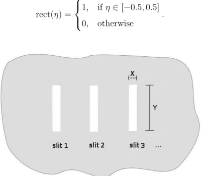
Imagine we have an opaque screen with D rectangular slits, each having a very thin film that controls its complex transmission coefficient. That is, the film at each slit controls both the field amplitude that is transmitted and phase that it gains, as depicted in figure1.1. Thus the transmission [38] function of this screen over the plane is given by
t(x, y) =
D
X
i=1
tieiφirect
x−xi
X
recty
Y
, (1.2)
where ti is the real transmission coefficient, φi the phase gain and xi the center of the ith
slit; also, X ans Y are widths of the slits in the xand y directions, respectively, and rect is the rectangle function, given by
rect(η) =
1, if η ∈[−0.5,0.5]
0, otherwise . (1.3)
Figure 1.1: Screen with D slits; its transmission functions is given by equation (1.2).
Now if we impinge a monochromatic plane wave of frequency ω and amplitude E0 on
this screen, propagating in thez direction, the field immediately after the screen (supposed atz = 0) will be
Et(x, y, t) =t(x, y)E0e−iωt (1.4)
=e−i ω t
D
X
i=1
tiei φiE0rect
x−xi
X
recty
Y = D X i=1
tiei φiEi(x, y, t). (1.5)
4 1.1. Mimicking quantum states with an electromagnetic field
of each ci, and the single-slits fields
Ei(x, y, t) = E0e−i ω trect
x−xi
X
recty
Y
(1.6)
playing the roles of the basis states |ii. This shows that, by controlling the transmission coefficients of each slit (making ti = |ci| andφi = argci), we can mimic an arbitrary state
|ψi.
Of course, equation (1.5) is an approximation. We did not use diffraction theory to find the transmitted field, we just used the approximation that it is given by the product of the transmission function and the incident wave. In fact, the vectorial theory of near field diffraction can be a quite hard subject. However, if we admit that the incident wavelength is much smaller than the dimensions of the slits, this is a good approximation.
Isomorphism between slit fields and quantum states
We have seen how an electromagnetic field can be similar to a qudit. Actually, we would like them to be so similar that any operation and any quantity defined for the quantum states can be also implemented or calculated for the slit fields. Mathematically, what assures this is possible is a relation called isomorphism.
Let us call the set of all possible slit fields H′. What we are claiming is that the
correspondence
h: H 7−→ H′
D
X
i=1
ci|ii 7−→
1
E0
D
X
i=1
tiei φiEi, (1.7)
with ti =|ci| and φi = arg(ci) is a isomorphism and thus preserves the structure of the
Hilbert space of the possible states|ψi, so that the space H′ of transmitted fields E
t is a
faithful copy2 of H. This is to say that h satisfies the following properties:
(i) it is a bijection3;
(ii) preserves linear combinations: h(αψ1+βψ2) = αh(ψ1) +βh(ψ2);
(iii) preserves inner products: hh(ψ1)|h(ψ2)i=hψ1|ψ2i;
2
We are claiming thathis anisomorphism between the Hilbert spaces; this is not surprising: one can check thatH′, which is generated by the slit fieldsEi, is indeed a Hilbert space ofD dimensions, just as H, and remember that a mapping that takes an orthonormal basis in one finite-dimensional Hilbert space to another orthonormal basis in the other will be an isomorphism.
3
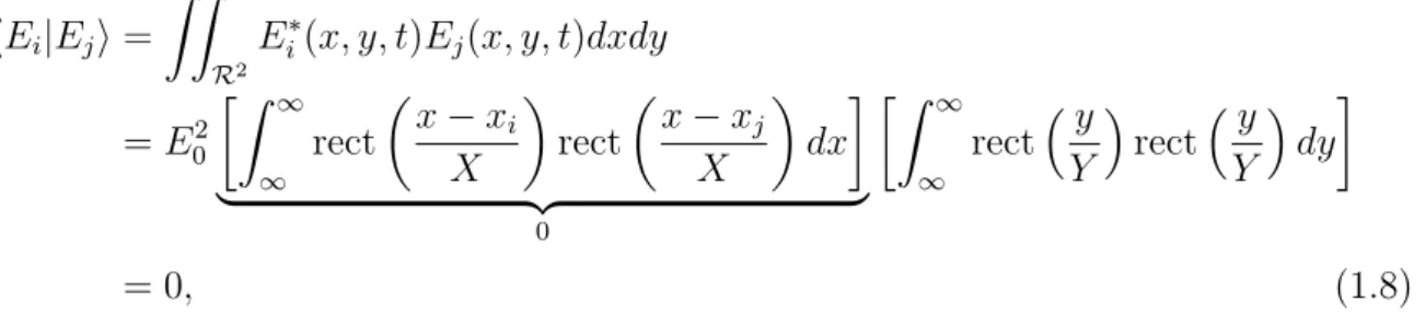
which are all straightforward to check; for property (iii), it is useful to note that the slit fields are orthogonal: if we let j 6=i, then
hEi|Eji=
Z Z
R2
Ei∗(x, y, t)Ej(x, y, t)dxdy
=E02
Z ∞
∞
rect
x−xi
X
rect
x−xj
X
dx
| {z }
0
Z ∞
∞
recty
Y
recty
Y
dy
= 0, (1.8)
where we have used the fact that the slits should have a separation bigger than their widths, X >|xi−xj|, and in this case the product of the rectangle functions inside the
first integral is zero for all x.
In order to get some appreciation for these three conditions, we can think of the possible “defects” that could arise in case our map did not satisfy them. Some defects are
depicted in figure 1.2. For property (ii), we have to keep in mind that we are trying to
simulate a quantum system through another physical system: in this second system, we want not only to encode states, but also mimic operators on the first system.
(a) (b)
Figure 1.2: Pictorial examples of: (a) a non-1-to-1 mapping (b) a non-surjective mapping.
• If h were not injective (one-to-one), we would have different states |ψ1i and |ψ2i mapped to the same fieldE1; it is as if in the process of mapping, we had lost points of the original space.
• If h were not surjective (onto), we would have fieldsE without correspondent states
|ψi; it is as if we have gained points through the process of mapping.
• If h did not preserve linear combinations, an important class of linear operators
on H would have to be mapped to non-linear operators in H′: let A be a linear
6 1.1. Mimicking quantum states with an electromagnetic field
operator in H′ defined by4
A′(E) =h◦A(ψ),
with E and ψ corresponding by E =h(ψ); if it happens that
h(αψ1+βψ2)=6 αh(ψ1) +βh(ψ2)
for some α, β, ψ1 and ψ2, we makeψ01 and ψ02 such thatAψ0i =ψi and thus
A′(αE01+βE02) = h◦A(αψ01+βψ02) =h(αψ1+βψ2)
6
=αh(ψ1) +βh(ψ2) = αh◦A(ψ01) +βh◦A(ψ02)
⇒A′(αE
01+βE02)6=αA′(E01) +βA′(E02).
• Ifh did not preserve inner products, some probability distributions calculated from a state|ψi would have a different value than that calculated with the corresponding field E: let |ψmi, |ψni, Em and En be such that Em=h(ψm), En =h(ψn) but
hEm|Eni 6=hψm|ψni;
we can analyse two cases to see that some distribution probability will be altered
because of this defect in h. We can look, for example, at the probability that we
have a positive result when applying on stateψβ the projective measurement onto
state ψα, which is given by P(α|β) =| hψα|ψβi |2, and the corresponding probability
P′(α|β) =| hE
α|Eβi |2.
1. If | hEm|Eni | 6= | hψm|ψni |, then the probabilities P(m|n) =| hψm|ψni |2 and
P′(m|n) = | hE
m|Eni |2 are clearly different.
2. If hEm|Eni=eiφhψm|ψni with φ not a multiple of 2π, then for the state
|+i= p 1
2 + 2 Re(hψm|ψni)
(|ψmi+|ψni)
we have
P(m|+) = 1
2 + 2 Re(hψm|ψni)
1 +| hψm|ψni |2+ 2 Re(hψn|ψmi)
,
P′(m|+) = 1
2 + 2 Re(hψm|ψni)
1 +| hψm|ψni |2+ 2 Re(eiφhψn|ψmi)
, (1.9)
4
which will also be different given that hψm|ψni 6= 0 (the case hψm|ψni = 0
and hEm|Eni= 0 is ruled out by the hypothesis hψm|ψni 6=hEm|Eni; the case
hψm|ψni= 0 andhEm|Eni 6= 0 falls in the previous item).
Therefore, it is very important for the fields of the form (1.5) to have the same mathematical structure as the pure quantum states, otherwise one or more of the problems mentioned above will take place.
As a final remark before we proceed to the next section, there are two simplifications we would like to introduce in the basis of slit fields (1.6). We can treat the slits as having infinite width in the ydirection, so that they behave as one-dimensional fields. Also, since the temporal behaviour is the same for all the slits, it can be factored out. Thus the single slit fields can be simplified to
Ei(x) = E0rect
x−xi
X
. (1.10)
1.2
Spatial qudits
Many of the applications we mentioned in the beginning of this chapter used single photons instead of the classical fields described above. It seems natural to think of the wavefront of the laser beam as being proportional to the probability amplitude of a single-photon multimode field [39]. Following this line of thought, we could represent the single-photon field in the one-dimensional position coordinate5 as
|ψi=
Z
ψ(x)|1xidx, (1.11)
where ψ(x) is its normalized transverse probability amplitude, which is proportional to the transverse spatial profile of the beam. The states |1xi are defined here as
|1xi= √1
2π
Z
ei kx|1kidk, (1.12)
in analogy to the Fourier transform of the Dirac delta function6; the states |1ki are the
single-photon, plane-wave modes.
5
The existence of a position operator for photons is a tough and ongoing debate; we are not recurring to a position operator to define the states|1xi, but rather using the well defined plane-wave states.
6
8 1.3. Spatial qudits
Let us imagine that this single-photon field is sent through a screen with a D-slit
transmission function
t(x) =
D
X
j=1 ˜
cjrect
x−ηja
X
, (1.13)
where the ˜cj are the complex transmission coefficients, a is the separation between the
slits, X is their width and ηj = (j −1)−(D−1)/2. The field immediately after the
screen will be
|ψti=C
Z
t(x)ψ(x)|1xidx (1.14)
=C D X j=1 ˜ cj Z
ψ(x)rect
x−ηja
X
|1xidx, (1.15)
where C is a normalization constant. Finally, if we assume that ψ(x) is constant across all the slits [say ψ(x) =ψ0], we can write the state as
|ψti= D
X
j=1
cj|ji, (1.16)
with cj = ˜cj/
q PD
i=1|c˜j|2 and
|ji= √1
X
Z
rect
x−ηja
X
|1xidx. (1.17)
The field states 1.16only represent the part of the field that is trasmitted through the screen, and do not account for the part that is reflected. Since this part is the one that can be detected by a detector after the screen, we say that these states arepostselected.
These are the spatial qudits [40], which are D-dimensional quantum systems on
their own right. As we have mentioned in the beginning of the chapter, they have been increasingly used as a resource for applications involving higher-dimensional states (cryptography, communication and fundamental tests, for example).
From what we have seen before, they are also isomorph to the slit fields (1.5), and by
extension also isomorph to any other D-level quantum system. Therefore, we can also use
them to simulate other quantum systems.
1.3
Loss of phase information
It is common to attribute more weight to the intensity than to the phase profile of a field. However, one striking example of the importance of the phase information was given by Eliyahu Osherovich [41] in his PhD thesis (see section 1.3.4), which we will reproduce now (but with two different characters).
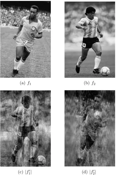
Imagine we get two grayscale pictures, which can be thought of as two real fields (in
the sense of having constant, zero phase profiles) f1 and f2. We can take their Fourier
transforms7 F
1 = |F1|eiφ1 and F2 =|F2|eiφ2, exchange their phase profiles and finally take the inverse transform of the resulting functions. This whole operation would be
f1 =F−1(|F1|eiφ1)
f2 =F−1(|F2|eiφ2)
−→
f′
1 =F−1(|F1|eiφ2)
f′
2 =F−1(|F2|eiφ1)
. (1.18)
Figure1.3 depicts the result of this process: in the end we get exchanged pictures. This
example illustrates how the phase information is important, as we could exchange the pictures themselves only by exchanging the phase profiles of their Fourier transforms.
Concerning the phase profiles of the slit fields, in equation (1.5) one can see that without controlling the phase of the field inside each slit region, it is impossible to generate all of the desired fields. Phase control is essential for this regard. Moreover, if we were to determine which field was generated with this scheme, we would need to measure the phase of the field in the slit regions8.
Photodetectors, however, do not record the phases of a field when it impinges on them, they only record intensities. To overcome this difficulty, several schemes have been devised to make the intensity at a given point dependent of the the field’s phase — for example by interfering the field under investigation with a plane wave reference field.
There is another such scheme, that takes advantage of the fact that the amplitudes of a Fourier transform depend on the phases of the original function. For instance, let us take the double-slit field
Et(x) =
1
√
2rect
x−a/2
X + e iφ √ 2rect
x+a/2 2X
, (1.19)
7
Throughout the text, we will be denoting the Fourier transform operation byF, and Fourier-transform pairs as the same letter with lower and upper cases; the Fourier transformF of a discrete functionf can be defined [42] as
Fk=
X
n
fne−i 2πkn/N 8
10 1.3. Loss of phase information
(a) f1 (b)f2
(c) |f′
1| (d) |f2′|
Figure 1.3: Illustration of the process given in equation (1.18); (a) and (b) show the original functions f1 and f2, while (c) and (d) show the absolute values of the resulting functions, f′
1 and f2′, after exchanging their phase in the Fourier domain. Besides adding some noise, the net result is to interchange the pictures, which illustrates how important the phase information is.
(a is the separation of the slits) which has the same amplitude in both slit regions, but has an arbitrary phase φin the second. According to the scalar theory of diffraction, after propagating a long distance, the diffracted field becomes a scaled Fourier transform of the original field [38]:
Ufar(x) = −i
λz
Z
U(η)e−i2λzπxηdη. (1.20)
where z is the propagation distance. Therefore, the far field corresponding to 1.19will be
Efar(x) = e
iΦ(z)
iλz
√
2X cos
2π2a
λz x+ φ
2
sinc
2πX λz x
where λ is the wavelength of the electromagnetic field. We are regarding the longitudinal distancez as a fixed parameter and the phase Φ(z) as a global phase.
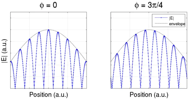
The amplitude profile of this field can be thought of as composed by two factors: a sinc envelope with a cosine oscillation. The phase φ has the role of displacing the oscillation pattern inside the envelope, as can be seen in figure 1.4
Figure 1.4: Amplitude profile of diffracted fields given in (1.21) for (a) φ = 0 and (b)
φ = 3π
4 . The phase difference φ between the slits causes the oscillatory pattern to shift inside the envelope. This illustrates that, in general, the amplitudes of a Fourier transform also depend on the phases of the original function; this fact is what underlies the algorithm we will see in the next chapter.
The dependence of the Fourier amplitudes on the original function phases is not trivial. In order to use the phase information that is somehow “buried” in the Fourier amplitudes, we have to resort to numerical algorithms, which we will discuss in the next chapter.
1.4
Fidelity between two quantum states
Later on we will be interested in quantifying how similar two quantum states are, and we will be using a measure called fidelity. The fidelity between two pure state |ψi and |φi is defined by [9]
̥(φ, ψ) =| hφ|ψi |. (1.22)
12 1.4. Fidelity between two quantum states
special case), the angle θuv between two unit vectors uand v is defined by
cosθuv =hu|vi, (1.23)
so that the fidelity between the two pure states |ψi and |φi is just the absolute value of the cosine of their angle9.
It is easy to see that when the first state lies on the subspace generated by the second (and thus their angle is either 0 or π), their fidelity equals one, and that when it lies on the subspace orthogonal to the second, their fidelity equals zero. Also, in intermediate situations the fidelity will lie between 0 and 1.
9
Phase retrieval algorithms
In the last chapter we have seen that the phase of a function and the amplitudes of its Fourier transform are related, though this relation is not trivial. In this chapter, we are going to see a few numerical algorithms that take advantage of this fact in order to solve the phase retrieval problem. For now, we will be more concerned in explaining the general features of the algorithms and leave the specific adaptations we made for our experimental setup to the next chapter.
2.1
The Gerchberg-Saxton algorithm
In 1972, Gerchberg and Saxton published an iterative algorithm to solve the phase retrieval problem in the context of electron microscopy [43]. In their experiments, an electron beam was impinged onto a sample which then scattered it, and assessing the scattered wavefunction of the electrons in the beam gave information about the sample object [7]. The electrons in the beam would propagate until they reach a two-dimensional detector, which would record a signal proportional to the intensity profile |ψ(x)|2 of the electron
beam 1. By controlling the current in electromagnetic lenses and thus tuning a magnetic
field that the beam had to transpose, they could control the propagation of the electron
beam. Specifically, they could make the plane where the detector lied an object plane or
a Fourier plane, just as with optical lenses. That is, they could make the wavefunction
at the detector plane the same as immediately after the sample, when the object plane
configuration was being used, or they could make it equal its Fourier transform with the
Fourier plane configuration.
Having the measured intensity profiles |f(x)|2 and |F(u)|2 of the Fourier transform
1
Even thoughxis a two-dimensional variable at this point, we will omit the vector notation because our work was done with one-dimensional functions, and the algorithm can be applied in the very same way.
14 2.1. The Gerchberg-Saxton algorithm
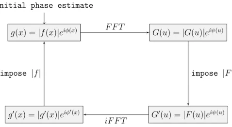
pair f −F at hand, one iteration of the Gerchberg-Saxton algorithm proceeds in four
steps:
Gerchberg-Saxton algorithm
(i) make an estimate φ(x) of the phases in the object domain, then
build an estimate g(x) =|f(x)|eiφ(x) of the function f;
(ii) take the Fourier transform of the estimate g to find G(u) =
|G(u)|eiψ(u);
(iii) correct the amplitudes of the Fourier transform G, but keep its
phases: G′(u) =|F(u)|eiψ(u);
(iv) take the inverse Fourier transform ofG′ to arrive at a new estimate
g′(x) = |g′(x)|eiφ′(x) of f.
By the end of step (iv), the new phase estimate of f is of courseφ′(x) = arg(g′(x))).
In the first iteration, we should start the algorithm using a random phase estimate in step (i) or an educated guess, if we have enough prior knowledge. But by the end of an iteration, we feed the phases φ′(x) of the new estimate g′ back into step (i) and start
another iteration. Thus, step (i) imposes the object-domain amplitudes |f(x)| at g′, in
a similar fashion to what step (iii) does in the Fourier domain. The iterative process is illustrated in figure 2.1.
g(x) =|f(x)|eiφ(x)
Initial phase estimate
G(u) =|G(u)|eiψ(u)
F F T
G′(u) =|F(u)|eiψ(u)
impose |F|
g′(x) =|g′(x)|eiφ′(x)
iF F T
impose |f|
Figure 2.1: Gerchberg-Saxton iterative algorithm.
To keep track of the progress of the algorithm, it is useful to define the object-domain normalized error:
Eo =
P
x(|g′(x)| − |f(x)|)
2
P
x|f(x)|2
This is just the squared residual of the amplitudes of the estimate function g′ at the
end of one iteration, normalized by the total object-domain intensity, and is calculated
repeatedly by the end of each iteration. Since step (i) will change the amplitudes of g′
but not its phases, the sum in the denominator is also a measure of the correction our estimate will suffer when the next iteration begins, and thus a measure of how far we are from the answer in the current iteration.
The iterative process is repeated until a numerical criterion is satisfied, for example, a certain number of iterations being reached. Another common choice is to repeat the iterations until the difference between errors in successive iterations is smaller than a fraction of the error in the current iteration. By the end, the algorithm should reach a good estimate of the phase off.
2.1.1
Some intuition on the workings of the Gerchberg-Saxton
algorithm
At first, it might not be obvious why this algorithm works at all. But one has to remember that by changing the amplitudes in either the Fourier or the object domains, we also change both the amplitudes and phases in the other domain, since these are inter-related. By making successive modulus impositions in steps (i) and (iii) of the algorithm, we are actually correcting the phase estimate φ(x) until it (hopefully) converges to the actual phase of the function f.
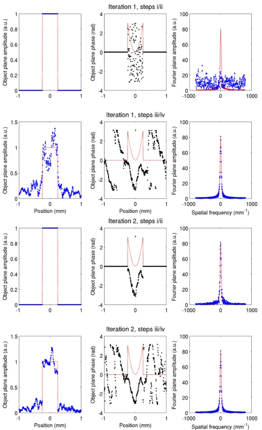
In figures 2.2 and 2.3, we illustrate this process with the results of the first iterations of the algorithm when ran with the chirp function
f(x) =ei16πx2rect(x). (2.2)
In these figures, the red full lines represent actual values of phase or modulus, while the black or blue dots show those quantities in the current estimate of the algorithm.
The first row of figure 2.2 shows (from left to right) |g|, arg(g) and |G| obtained in steps (i) and (ii) of the first iteration. One can see that, in spite of having the correct
object-domain amplitudes, the random phases of g give its Fourier transform a spectrum
that resembles white noise. In the second row there are (from right to left) plots of|G′|,
arg(g′) and |g′| obtained after steps (iii) and (iv) of the same iteration. It is possible to
see that by imposing the correct Fourier-domain amplitudes|F| made the object-domain
phase estimate much less random than it was initially.
The third and fourth rows in figure 2.2 show plots of the same quantities as in the
16 2.1. The Gerchberg-Saxton algorithm
Figure 2.2: Modulus and phase profiles of estimatesg andg′, and modulus profile ofGand
G′ for iterations 1 (first two rows) and 2 (last two rows) of the GSA; the target function
18 2.1. The Gerchberg-Saxton algorithm
and the phase estimates now start to resemble the actual phase profile.
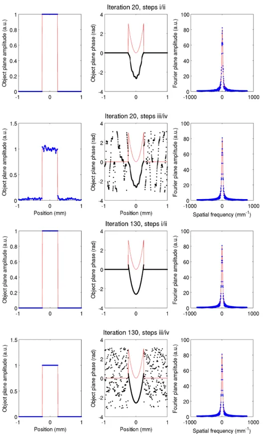
Figure 2.3 top two rows shows the same quantities described above, but now for
iteration 20. By now, |g′| seems quite close to the actual values of|f|. The object-domain
phases resemble the original values, but they are vertically shifted due to a global phase of the estimate with respect to the actual phases arg(f), which is actually not a problem.
Finally, figure 2.3 bottom two rows shows these quantities once again in iteration 130. The phase estimate is now quite close to the actual values in the region with non-zero amplitudes (apart from the constant phase shift) and |g′| is also close to the rectangle
function.
2.1.2
Weak convergence of the Gerchberg-Saxton algorithm
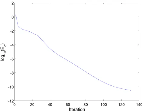
One striking feature of the Gerchberg-Saxton algorithm is that the error Eo [given in
equation (2.1)] never increases after one iteration, it can only decrease or stay unchanged. We say thereafter that the Gerchberg-Saxton algorithm is weakly convergent. For enstance, figure 2.4 shows the value of log10(Eo) at each iteration of the previous example with the
chirp function.
Figure 2.4: Progression of log10(Eo) when the GSA was run with the chirp function
(equation (2.2) and figures2.2 and 2.3).
Preliminary definitions
The object-domain error has been defined in equation (2.1); following that definition, this error ink-th iteration is given by
Eo,k =
P
x(|gk′(x)| − |f(x)|)
2
P
x|f(x)|2
, (2.3)
but if we remember that in this algorithm arg(g′
k(x)) = arg(gk+1(x)) and that |gk+1(x)|=
|f(x)|, we can rewrite Eo,k as
Eo,k =
P
x|gk′(x)−gk+1(x)|2
P
x|f(x)|2
. (2.4)
Similarly, we can define the Fourier-domain error at iteration k as
EF,k =
P
u(|Gk(u)| − |F(u)|)2
P
u|F(u)|2
, (2.5)
and if we remember that arg(G′
k(u)) = arg(Gk(u)) and that |Gk′(u)| = |F(u)|, we can
rewrite it as
EF,k =
P
u|Gk(u)−G′k(u)|2
P
u|F(u)|2
. (2.6)
Weak convergence
Parseval’s theorem states [42] that for any function h, its total intensity and the intensity of its Fourier transform H are related by
X
x
|h(x)|2 = 1
N
X
u
|H(u)|2 (2.7)
with N the number of pointsxin the object-domain (and thus also in the Fourier-domain).
First we look at the alternative definition of Eo,k in equation (2.4), and use Parseval’s
theorem with h(x) = g′
k(x)−gk+1(x) to arrive at
Eo,k =
1
N If
X
u
|G′k(u)−Gk+1(u)|2 =
1
IF
X
u
|G′k(u)−Gk+1(u)|2,
where we have made Px|f(x)|2 =I
f andPu|F(u)|2 =IF =N If. However, for each u
we have that, among all the numbers in the complex circle of radius|F(u)|,G′
20 2.1. The Gerchberg-Saxton algorithm
closest complex number to Gk+1(u), since they have the same phase. Therefore we have
1
IF
X
u
|G′k(u)−Gk+1(u)|2 ≥
1
IF
X
u
|G′k+1(u)−Gk+1(u)|2
and thus
Eo,k ≥EF,k+1. (2.8)
On the other hand, we can use Parseval’s theorem with H(u) =G′
k+1(u)−Gk+1(u) to
get from equation (2.6)
EF,k+1 = 1
IF
X
u
|G′k+1(u)−Gk+1(u)|2 = 1
If
X
x
|gk′+1(x)−gk+1(x)|2.
Similarly, we note that, for each x, gk+2(x) is the complex number closest to gk′+1(x) among the numbers in the circle of radius |f(x)|, since they have the same phase. Hence
1
If
X
x
|gk′+1(x)−gk+1(x)|2 ≥
1
If
X
x
|gk′+1(x)−gk+2(x)|2
and therefore
EF,k+1 ≥Eo,k+1. (2.9)
From equations (2.8) and (2.9), we have finally that
Eo,k+1 ≤Eo,k, (2.10)
which completes the proof.
2.1.3
Nonuniqueness and local-minima stagnation problems
On one hand, the weak convergence of the Gerchberg-Saxton algorithm establishes that it is a rather safe algorithm, in the sense that the estimate in the end of each iteration will not be worse than the estimate at the end of the previous iteration in terms of the
error Eo. On the other hand, it also tells us that the algorithm is somewhat similar to
gradient-descent algorithms, in the sense that it can get stagnated at a local minimum of the error that is not the global minimum. This can happen because the algorithm cannot “climb out” from an eventual error “well”.
Another difficulty that one has to deal with is the nonuniqueness of solutions of the phase retrieval problem. It is known [1] that there are more that one transform-pairf−F
that conform to |f|and |F|in some situations — for example the conjugate pair f∗−F∗
the one-dimensional phase retrieval problem suffers more severely from non-uniqueness
than the two-dimensional problem, and that a priori information on the function can also
affect how severe the non-uniqueness will be. One way to avoid these two problems is to run the algorithm several times with different starting phase estimates, as we will discuss in the next chapter.
2.2
Fienup’s family of algorithms
In spite of being safe, the Gerchberg-Saxton algorithm (to which we will refer as GSA from now on), usually converges slowly. We will turn our attention to a family of variations of the GSA that was developed to improve its performance by J. Fienup [6]. One remark before we begin though: Fienup devised his algorithms for a version of the phase retrieval problem that is different from the one we are interested in. In our experiment, it is easy to assess both the moduli|f| and |F|. Fienup was confronting a problem with less prior information about f: Instead of |f|, what is known is only that f is real and non-negative. Therefore, we are presenting versions of the algorithms that are adapted to our problem. The best-performing algorithm of this family of variations, called the hybrid input-output algorithm [44], did not have such an adaptation (in fact, it would reduce to the so-called
input-output algorithm, which we are about to see), but the interested reader is encouraged to pursue it.
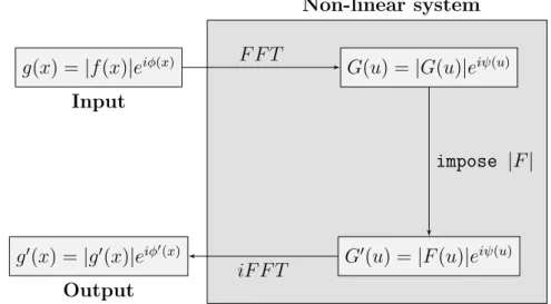
We can think of the last three operations in each iteration of the GSA (see figure 2.1and the box above it) as a non-linear system that receives gk as input and gives gk′
as output. Although the steps (ii) and (iv) are linear, step (iii) is not. Therefore this sequence of operations as a whole is non-linear (as sketched in figure2.5). Because of step (iii), g′
k already has the desired modulus in the Fourier-domain; it only lacks the correct
object-domain modulus in order to be a solution. Once we have calculated g′
k(x), we can
find the correction ∆gd(x) it needs in order to satisfy the object-domain constraint, that
is, we can find ∆gd so that|gk′(x) + ∆gd(x)|=|f(x)|. For example, one possibility is
∆gd(x) = −gk′(x) + |
f(x)|
|g′
k(x)|
g′
k(x), (2.11)
but the question then is how to change the input gk so that the output gk′ receives this
desired correction.
After running some iterations of the GSA, one would expect to be somewhat close to a solution, so the desired correction ∆gdshould be small. However, when one makes a small
22 2.2. Fienup’s family of algorithms
Non-linear system
g(x) = |f(x)|eiφ(x)
Input
G(u) = |G(u)|eiψ(u)
F F T
G′(u) = |F(u)|eiψ(u)
impose |F|
g′(x) = |g′(x)|eiφ′(x)
Output iF F T
Figure 2.5: Steps (ii), (iii) and (iv) of the Gerchberg-Saxton algorithm as a non-linear system.
so the input
gk+1(x) = gk(x) + ∆g(x) (2.12)
will give as output
g′k+1(x) = gk′(x) +α∆g(x), (2.13)
whereαis the proportionality coefficient between the perturbations, which is characteristic of the non-linear system. Therefore, by choosing ∆g(x) =α−1∆g
d(x) we can induce the
desired correction in g′
k.
The difficulty in this error compensation approach is that the exact value of α is hard to assess, as it depends on the statistics of|F(u)| and on the current solution estimate
gk′ [6]. This means the coefficient can change as we get closer to the solution or even
depend on the function one is trying to reconstruct. It is possible to estimate the value of
α−1 numerically as reported in [44]: one can make several runs from the same starting
phase estimate, each with a different value of β (an estimate for α−1) and all with the
same total number of iterations, and then compare the error curves to determine which β
value gave the algorithm the best error progression.
It is also possible to make an estimate of the value of β through the expected value
h|F|/|G|i, as shown in the appendix of [6]. Such an estimate can help in determining a suitable testing range for β.
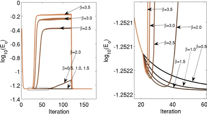
We made an estimate of the optimal value for β by generating several curves of Eo
against the iteration number (shown in figure 2.6), following the method we will describe
variation (which we will see very soon), and then 50 more iterations of the GSA. The first iterations with the GSA were intended to make the estimate somewhat close to an answer. The last were used because it has been reported [44] that Fienup’s family of variations
might increase the error Eo while actually improving the image quality; it could be the
case that one of the higher-error estimates was actually better in a visual criterium, so that running a few GSA iterations again would place its error below the other ones. This was not the case here, though2.
To generate the curves in figure 2.6, we ran the algorithm several times with a fixed
initial phase estimate, but each time using a different value for β. At the left figure, one can see that too high values of β (namely β = 2,2.5, 3 and 3.5) made the error increase after some iterations, meaning that the algorithm was unstable with those values. On the other hand, at the right figure, one can see that the lower values of β did not suffer from this instability, and that β = 1.5 gave the fastest decreasing curve. We chose to use
β = 1.3 in our routine in order to have a safety margin.
Figure 2.6: Numeric method for estimating the best value for β; (Left) Eo vs. iteration
number for several values ofβ; (right) zoom at the beginning of non-GSA iterations. The
valueβ = 1.5 gave the fastest-decreasing curve without making the algorithm unstable,
and was therefore the best tested value.
With an estimate β of α−1 at hand, the first variation of the GSA would be to correct
gk byβ∆gd [see equation (2.11)] when starting iteration k+ 1:
2
24 2.2. Fienup’s family of algorithms
Input-output algorithm
• proceed with steps (i) to (iv) of the GSA;
• correct the estimate gk(x) by β∆gd:
gk+1(x) = gk(x) +β
|f(x)|
|g′
k(x)|
−1
g′k(x).
This is the so-called input-output algorithm, in which we compensate the input to the
next iteration based on the error of the current output.
Another variation of the GSA is the output-output algorithm, which relies on another
characteristic of the non-linear system (figure 2.5). If an output g′(x) is fed as input to
the system, the new output is again g′(x), since the third step will not make any change
in F[g′]. Therefore, we can consider every output as resulting from itself as input. Hence
we can use a perturbed input similar to (2.12),
gk+1(x) =gk′(x) + ∆g(x), (2.14)
to get the same output as in equation (2.13). Following the same reasoning as before and making ∆g =β∆gd [see equation (2.11)], we arrive at another variation of the GSA,
called output-output algorithm:
Output-output algorithm
• proceed with steps (i) to (iv) of the GSA;
• correct the output g′
k(x) by β∆gd:
gk+1(x) = gk′(x) +β
|f(x)|
|g′
k(x)|−
1
g′k(x).
It is interesting to note that the output-output algorithm is equivalent to the GSA when
we choose β = 1. Thus we can think of the GSA as a special case of the output-output
algorithm, but with a suboptimal parameter value since it converges somewhat slowly.
We can also infer that, while β = 1 might not the best value, it is probably not very
far off, since the GSA is still very reliable. Larger values of β can make this family of
variations converge faster, as they would make more significant changes to the input after each iteration. However, excessively large values might make them unstable, as we have seen in figure2.6.
Phase retrieval algorithms for spatial
qudits: Problem-specific adaptations
In the last chapters we have seen how the phase retrieval problem arises when we try to determine the state of a spatial qudits, and also a few numerical algorithms that could solve it using object- and Fourier-plane intensity measurements. Our discussion so far was about the general working of these algorithms, but in this chapter we shall turn our attention to the specific adaptations we had to make so they could suit our problem.
3.1
Match of frequencies by expanding object-domain
amplitude vector
In the last chapter, we saw some algorithms to reconstruct a (complex) field given its modulus profile and that of its Fourier transform. In other words, these two profiles are the input that the algorithm uses, and therefore are the quantities we need to measure.
In our experiment, the Fourier transform of the qudit field was obtained by means of a lens. It can be shown that, in the Fraunhoffer diffraction regime, the field at a distance
lf after a spherical lens of focal length also equal to lf is given by [38]
Ufo(x) = −i
λlf
Z Z
Uim(u)e−i 2π
λlf(ux)du, (3.1)
with Uim being the field at a distance lf before the lens and λ the light wavelength. In
other words, the field at the output focal plane corresponds to a scaled Fourier transform of the field at the input focal plane. In our apparatus, the field Uim was a spatial qudit field of the form (1.5). Uim will play the role off in the phase retrieval problem, while
Ufo will play that of F (see chapter 2).
28 3.1. Match of frequencies by expanding object-domain amplitude vector
We placed a lens with its input focal plane over the plane where the qudit field Uim
was prepared, and set a camera at the output focal plane, so that it measured the Fourier transform intensities of the qudit field (we will discuss the experimental setup in more details in the next chapter). Each pixel of the camera measured the intensity of the field that was entering it; therefore, our experimental measurement gave us a vector of Fourier amplitudes, sampled at the positions
x(fon) =n∆xfo, n=−
Nfo 2 , . . . , Nfo 2 , (3.2)
where ∆xfo is the camera pixel size and Nfo is the number of pixels in the image. Our
camera had a pixel size of ∆xfo = 5.2µm and the images had up to 1268 pixels, the size of the camera. According to equation (3.1), the field Ufo at each position x(fon) corresponds to the Fourier transform at the spatial frequencies
p(fon) = 2π
λlf
x(fon) = 2π
λlf
∆xfon. (3.3)
However, the discrete Fourier transform (DFT) of a vector V(j) with N entries,
sampled at positions x(j) =j∆x, is another vector with N entries VDFT(n), given by [42]
VDFT(n) =
⌈N/2⌉ X
j=−⌊N/2⌋
V(j)ei2Nπjn=
⌈N/2⌉ X
j=−⌊N/2⌋
V(j)eiN2∆πxnx(j)
, (3.4)
which is sampled at the spatial frequencies
p(DFTn) = 2π
N∆xn, n=−
N 2 , . . . , N 2 . (3.5)
These frequencies p(DFTn) are the ones the computer will be using in its internal
rep-resentation while running the F F T andiF F T routines. But since we will be imposing
experimentally measured amplitudes during step (iii) of the GSA (see section 2.1), it is
essential that these frequencies match those corresponding to the sampling of the camera pixels, otherwise we will be imposing Fourier amplitudes at the wrong values of frequency. Therefore, the frequencies (3.3) and (3.5) need to match. This will be achieved as long as we have
N = λlf ∆xfo∆x =
λlf
(∆x)2. (3.6)
Imposing this value forN meant to change the size of the vectorV(j) — whose role is played by the spatial qudit field Uim. By usingλ = 691 nm,lf = 0.3 m and ∆x= 5.2µm,
one would conclude thatN = 7666 pixels were needed in our image, while our camera had
only 1268, and thus we needed to extend our object-domain image1. This was achieved
by placing 3199 zeroes before and another 3199 after the vector of measured intensities (these are called the trailing zeroes).
Since the spatial qudit fields are zero-valued outside the slit regions, this procedure did not compromise the results, since the object-domain camera was wide enough to capture all the slits. In oher words, completing the object-domain vector with trailing zeroes mimics what the camera should have measured if it had more pixels.
3.2
Partial imposition of Fourier-domain amplitudes
When dealing with other variations of the phase retrieval problem, in which one has
different a priori information about f andF, the usual approach is to modify step (iii)
and the update of gk in the GSA. Instead of imposing|f| and |F| as in our case, one can
simply impose those conditions whichf and F are known to satisfy.
In its original form, the GSA works with known moduli |f| and |F| across the whole image; this rather strong condition can be grasped in the proof of the weak convergence
(section2.1.2), which uses Parseval’s theorem and therefore presupposes that the sums
over x and u, in the calculus of the errors Eo or EF, span the whole object or Fourier
domain. This entails that |f(x)| and |F(u)| are known at every point in both domains. Our amplitude measurements in the Fourier domain, however, yielded us only up to
1268 pixels (the reason why we are saying up to will be clear soon), while the whole
domain had 7666. We only knew the values for |F| at the central portion of the spectrum
therefore. Even though this is not the case corresponding to the original GSA, we carried our iterations with a slight modification in step (iii): the imposition of|F|was onlypartial,
in the measured region. We let the values of the estimate G float freely outside that
region.
Before running our routine on experimentally measured data, we made several tests
using simulated values. In those tests, we used |F| vectors with 1268 entries, but this
limitation in the domain did not seem to be too serious, as only a small part of the intensity in the Fourier plane fell off of the region in which |F| was known. However, our experimental data had only 608 pixels, and the intensity falling off the measured region
1
30 3.4. State estimation from the algorithm results
was considerable. To overcome this difficulty with the experimental data, we had to resort to the modification described in section3.6.
3.3
State estimation from the algorithm results
The output of the phase retrieval algorithm was a vector g with many complex entries
(namely 7666). This vector corresponded to an optical field of the form (1.5), expected
to be piecewise constant. We built the estimated state |ψ˜gi corresponding to g with
the median of the amplitudes and phases inside each slit region. That is, we built the estimated state as
|ψ˜gi=
1 C ˜
A1ei ˜
φ1
˜
A2eiφ˜2 ... ˜
ADeiφ˜D
, (3.7) where ˜
Aj = median
x∈Xj |
g(x)|, (3.8)
˜
φj = median
x∈Xj
arg g(x) , (3.9)
Xj denotes the j-th slit region for j = 1, . . . , D and C =
qP
jA˜2j is a normalization
constant.
3.4
Reinitialization and post-selection of estimates
As we have seen in section 2.1.2, the GSA is weakly convergent: an iteration of this
algorithm cannot make the error Eo increase. This characteristic makes the GSA both
safe, in the sense that it will not worsen any estimate g in terms of Eo, and vulnerable to
local minima, since it cannot climb out an error well in case it falls in.
One possibility to avoid this difficulty is to run the algorithm several times with the same data, using a different initial phase estimate each time. One would expect that the algorithm does not get caught in the same local minimum in all the runs, hence one can collect several final estimates and select the one with the smaller error Eo. The
reinitialization and post-selection process is illustrated in figure3.1, which we will explain in better detail now.
(a)
(b)
Figure 3.1: Solutions found by our algorithm when simulating a D= 10 qudit state with
32 3.5. Reinitialization and post-selection of estimates
times with the corresponding simulated data. First, we run the algorithm 10000 times and just saved the estimates it arrived when the stopping criterium was met (absolute change in the error being less than 10−8; the errors themselves were of the order of 10−3). There was no selection of the estimates whatsoever in this first test, shown in figure 3.1(a), as we were trying to discover how serious the problem of local minima was. After the
algorithm converged to an estimate, we calculated its fidelity ̥ (section 1.4) with the
original state, and made a histogram of fidelities and errors. One can see that there are several count peaks across the histogram, implying that the algorithm got stuck at several
estimates that are local minima. The estimate with Eo ≈ 10−3.5 and ̥ ≈ 1, the error
global mimimum and fidelity maximum, was still the most probable peak, being reached about 1400 times in the 10000 runs.
Next we repeated the process, but now selecting the best among 20 estimates (which means to reinitialize the algorithm 19 times). In this manner we could check how well the post-selection strategy would perform, in particular if this number of reinitializations would be reliable. Also, we only saved 1000 estimates instead of 10000, because of the
increase in the computing time. As figure 3.1(b) shows, this strategy yielded the error
global minimum estimate very reliably, as the histogram has now only one peak. Most importantly, the error global minimum was also the fidelity global maximum (being very close to 1), so that this approach in fact helped the algorithm to arrive at better state estimates.
As a final remark, we note that a histogram such as the one in figure 3.1(a) can aid
in estimating how many reinitializations are needed for the algorithm to have a given
reliability figure. If the global minimum peak has a fraction p of all the estimates (in
our case, for example, p amounted roughly to 0.14, as the peak had 1400 estimates in a
total of 10000), and if we admit that the algorithm converges independently to each local minimum (which is plausible, since reinitializing it amounts to taking another random
phase estimate), then the probability that no estimate in Nest will fall in the global
minimum will be
P(no global min.|Nest) = (1−p)Nest, (3.10)
which is monotonically decreasing with Nest. Hence, if a reliability figure δ is desired, one needs to select among a number of estimates such that 1−P(no global min.|Nest)> δ, which translates to
Nest >
log(1−δ)
3.5
Some results with simulated data
Before running the algorithm with our experimental data, we used simulated data to check if it was working properly. In fact, the adaptations we described so far were developed during this stage. Our greatest worry was that the sampled region in the Fourier domain was too small, and the data we would have to feed the algorithm would be insufficient for it to find good estimates.
In this stage we fed the algorithm data corresponding to perfectly rectangular slits and their corresponding interference pattern, without including imprefections from realistic experiental situations such as vignetting [38] from the lenses or detection noise. Another aspect of the simulated data was its width: the simulated amplitude vectors had 1268 pixels. However, the experimental data was more limited, having only 608 pixels in the Fourier-domain amplitude vector. We will discuss how we dealt with this in the next section. Figure3.2 depicts a typical result obtained with the algorithm at this stage. For
Figure 3.2: Result with simulated data for a D = 4 state: object-domain amplitudes