Wang-Landau Sampling of an Asymmetric Ising Model: A Study of the Critical
Endpoint Behavior
Shan-Ho Tsaia,b, Fugao Wanga,∗, and D.P. Landaua
aCenter for Simulational Physics, University of Georgia, Athens, GA 30602, USA bEnterprise Information Technology Services, University of Georgia, Athens, GA 30602, USA
Received on 6 October, 2005
We use the Wang-Landau algorithm to calculate a density of states for an asymmetric Ising model on a triangular lattice with two- and three-body interactions in an external field. An accurate density of states allows us to determine the phase diagram and to study the critical behavior of this model at and near the critical endpoint. We observe a divergence of the curvature of the spectator phase boundary at the critical endpoint in accordance with theoretical predictions.
Keywords: Critical endpoint; Wang-Landau sampling; Ising model; Triangular lattice; Three-body interaction
I. INTRODUCTION
A critical endpoint (CE) is a point in the phase diagram where a critical line meets and is truncated by a first-order transition line. Critical endpoints appear in the phase diagram of many physical systems such as binary fluid mixtures, super-fluids, binary alloys, liquid crystals, certain ferromagnets, etc. The bulk critical exponents are believed[1] to be unchanged at CE, but this has not been checked beyond phenomenologi-cal theory and renormalization phenomenologi-calculations.[2] (However, the universal character of a double critical endpoint has been nu-merically determined from extensive Monte Carlo simulations [3].) Moreover, a new singularity in the first-order phase tran-sition line was shown to arise at CE. [1, 4] This prediction was confirmed by Fisher and Barbosa’s phenomenological studies on an exactly solvable spherical model[4].
The critical endpoint behavior in a symmetrical binary fluid mixture was studied by Wilding[5] using a large scale Monte Carlo simulation[6] with multicanonical[7] and his-togram reweighting[8] methods. He showed the first numer-ical evidence of a singularity at CE for the diameter of the liquid-gas coexistence curve and for the curvature of the spec-tator phase boundary.
In this paper we study a two-dimensional Ising model on a triangular lattice with two- and three-body interactions in a uniform external field. For a range of coupling parame-ters, this model has a critical endpoint.[9] We use the Wang-Landau sampling technique[10, 11] with a two-dimensional random walk to determine the density of states and thereby the phase diagram with great accuracy. The high resolution of this simulation allowed us to compute the curvature of the first-order phase transition line and observe the singularity that arises at CE. We were also able to determine the criti-cal exponents along the second-order transition line and we confirm that these exponents indeed do not change as CE is approached.
∗Current address: Intel Corporation, PC1-105, 44235 Nobel Drive, Fremont,
CA 94538
II. MODEL AND METHODS
The model considered here is described by the Hamiltonian
H
=−J∑
<i j>SiSj−P
∑
<i jk>SiSjSk−H
∑
iSi (1)
whereSi=±1 is an Ising spin on siteiof a two-dimensional triangular lattice, <i j> denotes pairs of nearest-neighbor spins, and<i jk>represents the three spins on the elemen-tary triangles. The parametersJandPare two- and three-body nearest-neighbor spin couplings, respectively, andHis an ex-ternal magnetic field. The model is asymmetric because the Hamiltonian is not invariant whenH→ −H. Periodic bound-ary conditions are used in this work.
Previous Monte Carlo simulations by Chin and Landau [9] showed that this model exhibits critical endpoints for a range of values of parametersJandP. In particular, there is a crit-ical endpoint in theT andHphase diagram whenJ=1 and P=2; this is the set of parameters used in this paper. We per-form Wang-Landau sampling[10, 11] to determine the phase diagram of this model and to study its behavior at the phase transition lines and at the critical endpoint.
Unlike conventional Monte Carlo methods[6] that directly generate a canonical distribution at a given temperatureT, the Wang-Landau method estimates the density of states directly and accurately via a random walk that produces a flat his-togram in the random walk parameter space. Wang-Landau sampling has proven very useful and efficient in many differ-ent applications, including studies of complex systems with rough energy landscapes. For example, this method has been used in studies of a Potts antiferromagnet[12], random spin systems[13], quantum systems[14–16], fluids[17, 18], binary Lennard-Jones glass[19], liquid crystals[20], polymers[17, 21], proteins[22, 23], other molecular systems[24, 25], atomic clusters[26], optimization problems[27], and combinatorial number theory[28]. Generalizations and further studies of this sampling technique have also been carried out by several authors[29–33].
glass problem [11]. We restrictP/Jto an integerm(m=2 in this paper); therefore we can rewrite the Hamiltonian in Eq. (1) as a sum of two parts,
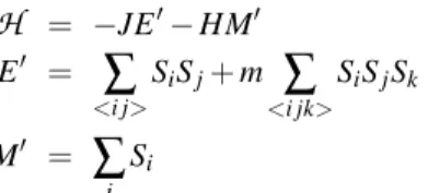
H
= −JE′−HM′ E′ =∑
<i j>
SiSj+m
∑
<i jk>SiSjSk (2) M′ =
∑
i Si
whereE′ is proportional to the energy due to the two- and three-body interactions, and M′ is the magnetization of the system. We perform a 2D random walk in theE′-M′ space using the Wang-Landau algorithm [10, 11] to estimate the density of statesg(E′,M′), which is defined as the number of spin configurations for any givenE′andM′. The estimate for g(E′,M′)is improved at each step of the random walk, using a carefully controlled modification factor, to produce a result that converges to the real value very quickly, even for large system sizes. The thermodynamic quantities can then be ex-tracted by applying canonical average formulas in statistical physics.
We provide a succinct description of the sampling method here, more details can be found elsewhere[10, 11]. At the start of the simulation, the density of states is unknown, so we simply setg(E′,M′) =1 for all possible(E′,M′). Then we begin our random walk inE′−M′ space by choosing a site randomly and flipping its spin with a probability proportional to the inverse of the density of states. If we denoteA′(E′,M′) andA′′(E′′,M′′)as the points before and after a spin is flipped, respectively, the transition probability fromA′toA′′is:
p(A′→A′′) =min
·g(A′)
g(A′′),1
¸
. (3)
If the point A′′(E′′,M′′) is accepted we multiply the ex-isting density of states by a modification factor f > 1, that is, g(E′′,M′′)→ f g(E′′,M′′), and we update the his-togramh of visited states, that ish(E′′,M′′)→h(E′′,M′′) + 1. If A′′(E′′,M′′) is not accepted, we update g(E′,M′)→
f g(E′,M′)andh(E′,M′)→h(E′,M′) +1.
We continue performing the random walk until the his-togram h(E′,M′)is flat inE′−M′ space. The modification factor f introduces a systematic error for the estimated den-sity of states. The magnitude of this error for ln[g(E′,M′)] is proportional to ln(f). To reduce this source of error, we systematically reduce the modification factor to a finer one using a function like fi+1= fi1/n (n>1) wherei here de-notes the number of iterations in the algorithm (each iter-ation is a 2D random walk in the E′−M′ space). To be explicit, when iteration i generates a flat histogram, we re-set the histogram to zero, and begin the next iteration with a new factor fi+1. We end the simulation when the mod-ification factor is smaller than a predefined value (such as
ffinal=exp(10−8)≃1.00000001 used here). To speed up the
convergence of the density of states to the true value, the initial modification factor was as large as f =f0=e≃2.71828..., andn=4 in our simulations. We perform the random walk on all possible(E′,M′)space with a single computer processor.
It takes from about a few minutes to 2 days on a 1.3 GHz Ita-nium processor to obtaing(E′,M′)for the lattices with linear sizesL=6 toL=30 used here.
We should point out that it is impossible to obtain a per-fectly flat histogram. A histogram may be considered flat if h(E′,M′)for all possible (E′,M′)is not less thanx% of the average histogram, wherex% is chosen according to the size and complexity of the system and the desired accuracy of the density of states. However, in this work we use a less stringent criterion: the histogram is considered flat when the number of entries larger than or equal to 2000 remains unchanged for L2×106spin flip trials.
With an accurate estimate of the density of statesg(E′,M′), we can calculate thermodynamic quantities at any temperature T, external magnetic fieldH, and couplingJfor the system with Hamiltonian given in Eq.(1). The spontaneous magneti-zation per lattice site as a function ofT andHis given by
M(T,H) =hMi=
∑ E′,M′
M′g(E′,M′)e−(−JE′−HM′)/kBT
N ∑
E′,M′g(E
′,M′)e−(−JE′−HM′)/kBT (4)
where we assumeJ=1>0 (ferromagnetic coupling),N=L2 is the number of lattice sites; andT is in unit of 1/kB (kBis the Boltzmann constant).
The susceptibilityχ(T,H)also can be calculated from the density of states by:
χ(T,H) =dM/dH=N(hM2i − hMi2)/kBT. (5)
III. RESULTS
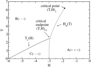
Figure 1 shows the phase diagram in theT anHplane for a finite lattice withL=30 (and the reader should remember that the entire phase diagram was obtained from a single simula-tion). There are three distinct phases with different values of magnetization atT =0: ferromagnetic phase A(+ + +) with M(0,H) =1 (all spins are up), ferromagnetic phase B( -) withM(0,H) =−1 (all spins are down) and ferrimagnetic phase C(- - +) withM(0,H) =−1/3 (the spins on two sublat-tices are down and on the other are up).
The transitions between A and B as well as between A and C are first order, whereas the phase transition between B and C is second order. The critical endpoint,(T,H)CE, is defined as the point where the critical lineTc(H)separating phases B and C meets, and is truncated by the first-order transition line Hσ(T)separating phase A from phases B and C. TheHσ(T)
line is also called the spectator phase boundary. At the end ofHσ(T)is a critical point(T,H)c. Our simulational results
Tc(H =−6) =0 and Hσ(T =0) =−3 are consistent with
the exact solutions at zero temperature and early simulational data [9].
-6 -5 -4 -3 -2 -1 0 H
0 1 2 3 4 5 6 7
T (T,H)CE
Tc(H)
Hσ(T)
B(- - -)
C(- - +)
A(+ + +) critical
endpoint critical point
(T,H)c
FIG. 1: Phase diagram forL=30.
define order parameters that are similar to those used for the Q=3 Potts model [34], because the degeneracy of the ground state in C phase is 3. We define two components (P1,P2) and a
vector order-parameterPfrom the magnetizations per site of the three sublatticesM1,M2andM3:
P1 =
1 2
µ
M1−
M2+M3
2
P2 =
√ 3
4 (M2−M3) (6)
P = q
P12+P22
P1(T,H),P2(T,H)andP(T,H)approach zero in the phases
A(+ + +) and B(- - -), and finite values in the ferrimagnetic phase C(- - +).
To calculate thermodynamic quantitiesP(T,H), we have to accumulate microscopicP(E′,M′)during the random walk in theE′-M′space. IfP(E′,M′)is the microscopic average value during a random walk at(E′,M′), the thermodynamic quantity P(T,H)can be calculated as:
P(T,H) =
∑
E′,M′P(E
′,M′)g(E′,M′)e−(−JE′−HM′)/kBT
∑
E′,M′
g(E′,M′)e−(−JE′−HM′)/kBT . (7)
The phase diagram in Fig.1 is determined by the locations where the susceptibilityχp(T,H) =dP/dHhas the maximum value for a given value ofTfor a lattice withL=30.
We determine the critical lineTc(H)separating phase B and C with great accuracy, except when this line reaches CE. It is very difficult to determineTc(H)near CE, because the first-order transitions are so strong. However,Tc(H)is a smooth line and we extend it from low values ofHto where it meets the first-order transition line. We then take this meeting point as an estimate of the critical endpoint for the finite latticeL. For L=30 we estimate the critical endpoint as(T,H)CE = (2.48±0.02,−2.93±0.02); this value will be used in the data analysis below.
The critical line Tc(H) for this asymmetric Ising model studied here should be in the same universality class as the two-dimensionalQ=3 Potts model, because the two mod-els have the same symmetry. We recall that the conjectured values[35] for the critical exponents of the latter model are α=1/3,β=1/9,γ=13/9, andν=5/6. In order to verify that our data are consistent with these conjectured exponents, we study finite size scaling of derivatives of the order parame-ter alongTc(H). Because the order-parameterPbehaves as P(T)∝|(T−Tc(H))/Tc(H)|βnear the critical lineTc(H), the
finite-size behavior ofdP/dT atTc(H)is
dP(L)
dT
¯ ¯ ¯ ¯T
c(H)
∝L(1−β)/ν (8)
The finite-size scaling behavior of the susceptibilitydP/dH at the critical line is
dP(L)
dH
¯ ¯ ¯ ¯
Tc(H)
∝Lγ/ν (9)
Figure 2(a) showsdP/dT alongTc(H)for several lattice sizes. Characteristic error bars shown for the L=30 data are obtained from several independent runs. In the inset of Fig.2(a), the absolute value ofdP/dT versusLat three criti-cal points in a wide region of external field (H=−4.8,−4.0 and−3.2) can be fitted well to the scaling form in Eq.(8) with (1−β)/ν=48/45≃1.07, where we used the conjectured critical exponents for the 2DQ=3 Potts model [35].
The susceptibilitydP/dHalongTc(H)is shown in Fig.2(b) for several values ofL. The finite-size behavior ofdP/dHin the inset of Fig.2(b) for different values ofHscale well ac-cording to the relation given in Eq.(9), using the 2DQ=3 Potts critical exponents γ/ν= (13/9)/(5/6)≃1.73. The finite-size scaling shown in the insets of Figs.2(a) and 2(b) confirms that the transition between phase C(- - +) and phase B(- - -) is in the same universality class as the 2DQ=3 Potts model. Moreover, these results show that the critical expo-nents do not change when we approach the critical endpoint along the critical lineTc(H).
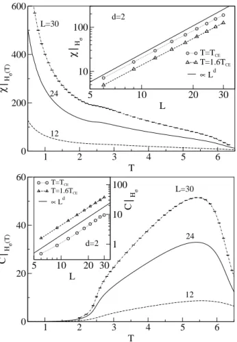
For the first-order transitions along Hσ(T), finite-size
analysis indicates that both at and away from CE the max-imum of thermodynamics quantities are proportional to Ld for finite-size systems (whered is the dimensionality of the lattice). In particular, the susceptibilityχ=dM/dH and the specific heatCscale as
χ(L)|Hσ(T) ∝ L
d
C(L)|Hσ(T) ∝ L
d (10)
Figures 3(a) and 3(b) show the susceptibility and the specific heat, respectively, alongHσ(T)for several lattice sizes. The
insets in these figures confirm that the scaling relations in Eq.(10) are satisfied both at CE and away from it (for example, atT =1.6TCE).
-4.8 -4.4 -4 -3.6 -3.2 H
-8
-6
-4
-2
0
dP/dT
Tc
(H)
5 10 L 20 30
1 4
dP/dT
T(H)c
H=-4.8 H=-4.0 H=-3.2
∝L(1-β)/ν
(1-β)/ν=48/45
L=30
24
12
-4.8 -4.4 -4 -3.6 -3.2
H 0
10 20 30 40
dP/dH
Tc
(H)
5 10 L 20 30
1 10
dP/dH
Tc
(H)
H=-4.8 H=-4.0 H=-3.2
∝Lγ/ν
γ/ν=26/15
L=30
24
12
FIG. 2: Dependence of (a)dP/dT and (b)dP/dH onHalong the critical lineTc(H)for several lattice sizes. The insets show the
sin-gularity in the respective thermodynamic quantities for three values ofHalongTc(H). The error bars in the insets are not larger than the
symbol sizes.
phase boundary has a very clear singularity at CE. According to a general finite-size scaling argument [1, 5], this curvature diverges at CE as
d2Hσ(T,L)
dT2 ¯ ¯ ¯ ¯CE
= cLα/ν (11)
where α andνare critical exponents defined on the critical lineTc(H). The lattice sizes used here are not large enough to give a good estimate of the scaling exponentα/νpredicted by theory. For a binary fluid mixture, Wilding[5] observed a clear divergence of the curvature of the spectator phase bound-ary; however the system sizes he considered in his simulations were also not large enough to determine the finite-size scaling exponent accurately.
IV. CONCLUSION
We used the Wang-Landau algorithm with a two-dimensional random walk to determine the density of states
1 2 3 4 5 6
T 0
200 400 600
χH
σ
(T)
5 10 20 30
L 10
100
χ
Hσ
T=TCE
T=1.6TCE
∝ Ld
L=30
24
12
d=2
1 2 3 4 5 6
T 0
20 40 60
C
Hσ
(T)
5 10 20 30 L
10 100
1
C
Hσ
T=TCE
T=1.6TCE
∝ Ld
L=30
24
12 d=2
FIG. 3: Dependence of (a) the susceptibilityχ=dM/dHand (b) the specific heat onT along the first-order phase transition lineHσ(T)
for several lattice sizes. The insets show the singularity in the respec-tive thermodynamic quantities atT=TCE and atT=1.6TCE along Hσ(T). The error bars in the insets are not larger than the symbol
sizes.
2 2.4 2.8 3.2
T 0.1
0.2 0.3
d
2 H
σ
/dT
2
L=9 L=15 L=18 L=21 L=30
FIG. 4: Singularity of the curvatured2Hσ/dT2of the spectator phase
g(E′,M′)for an asymmetric Ising model with two- and three-body interactions on a triangular lattice, in the presence of an external field. With an accurate density of states we were able to map out the phase diagram accurately and observe a clear divergence of the curvature of the spectator phase boundary at the critical endpoint. However, larger systems have to be stud-ied to obtain an accurate estimation of the scaling exponent of this divergence.
We show that the critical line separating phases B and C is indeed in the two-dimensionalQ=3 Potts universality class and that the critical exponents do not change along the critical
line. Thermodynamic quantities along the first-order line are shown to scale with lattice size asLdboth at and away from the critical endpoint.
Acknowledgments
We thank J. Plascak, J. S. Wang, M. M¨uller, K. Binder, H. Meyer, and C. K. Hu for helpful discussions and comments. Part of the simulations were performed on the Itanium cluster at SDSC. This work is partially supported by the NSF under Grants number DMR-0341874 and DMR-0307082.
[1] M. E. Fisher and P. J. Upton, Phys. Rev. Lett. 65, 2402 (1990);65, 3405 (1990); M. E. Fisher, Physica A 172, 77 (1991).
[2] T. A. L. Ziman, D. J. Amit, G. Grinstein, and C. Jayaprakash, Phys. Rev. B25, 319 (1982).
[3] J. A. Plascak and D. P. Landau, Phys. Rev E67, 015103(R) (2003).
[4] M. E. Fisher and M. C. Barbosa, Phys. Rev. B43, 11177 (1991); M. C. Barbosa and M. E. Fisher, Phys. Rev. B43, 10635 (1991); M. C. Barbosa, Phys. Rev. B45, 5199 (1992).
[5] N. B. Wilding, Phys. Rev. Lett.78, 1488 (1997); Phys. Rev. E
55, 6624 (1997).
[6] D. P. Landau and K. Binder,A Guide to Monte Carlo Meth-ods in Statistical Physics, second edition (Cambridge U. Press, Cambridge, 2005).
[7] B. A. Berg and T. Neuhaus, Phys. Rev. Lett.68, 9 (1992). [8] A. M. Ferrenberg and R. H. Swendsen, Phys. Rev. Lett.61,
2635 (1988);63, 1195 (1989).
[9] K. K. Chin and D. P. Landau, Phys. Rev. B36, 275 (1987). [10] F. Wang and D. P. Landau, Phys. Rev. Lett.86, 2050 (2001);
D. P. Landau and F. Wang, Comput. Phys. Commun.147, 674 (2002); D. P. Landau, S.-H. Tsai, and M. Exler, Am. J. Phys.
72, 1294 (2004); D. P. Landau and F. Wang, Braz. J. Phys.34, 354 (2004).
[11] F. Wang and D. P. Landau, Phys. Rev. E.64, 056101 (2001). [12] C. Yamaguchi and Y. Okabe, J. Phys. A34, 8781 (2001). [13] Y. Okabe, Y. Tomita, and C. Yamaguchi, Comput. Phys.
Com-mun.146, 63 (2002).
[14] M. Troyer, S. Wessel, and F. Alet, Phys. Rev. Lett.90, 120201 (2003).
[15] P. N. Vorontsov-Velyaminov and A. P. Lyubartsev, J. Phys. A
36, 685 (2003).
[16] W. Koller, A. Pr¨ull, H. G. Evertz, and W. von der Linden, Phys. Rev. B67, 104432 (2003).
[17] T. S. Jain and J. J. de Pablo, J. Chem. Phys.118, 4226 (2003). [18] Q. L. Yan, R. Faller, and J. J. de Pablo, J. Chem. Phys.116,
8745 (2002).
[19] R. Faller and J. J. de Pablo, J. Chem. Phys.119, 4405 (2003). [20] E. B. Kim, R. Faller, Q. Yan, N. L. Abbott, and J. J. de Pablo, J.
Chem. Phys.117, 7781 (2002).
[21] T. S. Jain and J. J. de Pablo, J. Chem. Phys.116, 7238 (2002). [22] N. Rathore and J. J. de Pablo, J. Chem. Phys.116, 7225 (2002). [23] N. Rathore, T. A. Knotts, and J. J. de Pablo, J. Chem. Phys.118,
4285 (2003).
[24] T. J. H. Vlugt, Mol. Phys.100, 2763 (2002). [25] F. Calvo, Mol. Phys.100, 3421 (2002).
[26] F. Calvo and P. Parneix, J. Chem. Phys.119, 256 (2003). [27] M. A. de Menezes and A. R. Lima, Phys. A323, 428 (2003). [28] V. Mustonen and R. Rajesh, J. Phys. A36, 6651 (2003). [29] C. Yamaguchi and N. Kawashima, Phys. Rev. E65, 056710
(2002).
[30] B. J. Schulz, K. Binder, and M. M ¨uller, Int. J. Mod. Phys. C13, 477 (2002).
[31] A. Huller and M. Pleimling, Int. J. Mod. Phys. C13, 947 (2002). [32] M. S. Shell, P. G. Debenedetti, and A. Z. Panagiotopoulos,
Phys. Rev. E66, 056703 (2002).
[33] B. J. Schulz, K. Binder, M. M¨uller, and D. P. Landau, Phys. Rev. E67, 067102 (2003).