Probability Distribution of the Order Parameter
P. H. L. Martins
1,2and J. A. Plascak
21Universidade Federal do Tocantins, Caixa Postal 111, 77001-970, Palmas, TO, Brazil
2Departamento de F´ısica, Instituto de Ciˆencias Exatas, Universidade Federal de Minas Gerais,
Caixa Postal 702, 30123-970, Belo Horizonte, MG, Brazil
Received on 1st December, 2003
The probability distribution of the order parameter is analyzed in order to obtain the criticality of magnetic systems. Monte Carlo simulations have been employed by using single spin flip Metropolis algorithm aided by finite-size scaling and histogram reweighting techniques. A method is proposed to obtain this probability distribution even when the transition temperature of the model is unknown. A test is performed on the two-dimensional spin-1/2 and spin-1 Ising model and the results show that the present procedure can be quite efficient and accurate to describe the criticality of the system.
1
Introduction
The order parameter distribution function has been proved to be a powerful tool for studying not only magnetic sys-tems [1-5], but also the liquid-gas critical point [6], the critical point in the unified theory of weak and electro-magnetic interactions[7], and the critical point in quantum chromodynamics[8]. For the specific case of magnetic sys-tems the order parameter can be chosen as the magnetiza-tion per spin, namely m = 1
N
N
i=1Si, where N is the
total number of spins andSi is the spin at sitei. In finite-size systems, the magnetizationmis a fluctuating quantity, characterized by the probability distributionP(m)[1, 2]. In Ising-like models undergoing a second-order phase transi-tion it is known that at temperatures lower than the critical temperatureTc, the distribution P(m) has a double peak, centered at the spontaneous magnetizations+mand−m. At temperatures greater thanTc,P(m)has a single peak at zero magnetization, and exactly atTc a double-peak shape is observed[1]. Analogously to the usual finite-size scaling assumptions [9], one then expects that, for a large finite sys-tem of linear dimensionLat the critical point,P(m)takes the form
P(m) =bP∗( ˜m), (1)
whereb=b0Lβ/ν,βandνare critical exponents,m˜ =bm, b0is a constant, andP∗( ˜m)is a universal scaling function,
normalized to unit norm and unit variance. Scaling func-tions, such as P∗, are characteristic of the corresponding
universality class. Systems belonging to the same universal-ity class share the same scaling functions. Thus, from the precise knowledge of P∗( ˜m)one can characterize critical
points and also identify universality classes. This is what has been done so far in the literature, with the distribution for the spin-1/2 Ising model being the standardP∗ function[4, 6]
for this universality class. For instance, it is shown in Fig. 1 the normalized distributionP∗( ˜m)for the two-dimensional
spin-1/2, spin-1, and spin-3/2 Ising model at criticality. Sim-ulations have been done on square lattices withL = 32at the exactTc for spin-1/2, atTc = 1.6935for spin-1, ac-cording series expansions [10] and Monte Carlo simulations [11], and atTc = 3.28794for the spin-3/2 model [11]. The universal aspect of these systems can be easily noted.
-2.0 -1.0 0.0 1.0 2.0
boLβ/νML 0.5
1.0
P
*
spin-1/2 spin-1 spin-3/2
Figure 1. Scaling functionP∗( ˜m)for the two-dimensional spin-1/2, spin-1, and spin-3/2 Ising model on square lattices withL= 32. Simulations were performed at the exactTc for spin-1/2, at
Tc = 1.6935 for spin-1, according series expansions [10] and
Monte Carlo simulations [11], and atTc = 3.28794for the
spin-3/2 model [11]. The error bars are smaller than the symbol sizes. After Ref. [11]
magne-tization ism, i.e.,
P(m) = Nm
NMCS
, (2)
whereNmis the number of times that magnetizationm ap-pears andNMCS is the total number of Monte Carlo steps.
To compute the normalized distributionP∗( ˜m)via Eq. (1)
one has to evaluate the pre-factorb. This can be easily done by noting thatb = 1/σ, whereσis the square root of the magnetization variance (σ2=m2 − m2). Thus, one
ob-tains the universal functionP∗( ˜m)by simply rescaling the
magnetization and by using Eq. (1).
In general, the probability distribution is used for study-ing models in which the critical temperature or even the dis-tribution function is exactly (or high-precisely) known. That is in fact what has been done in the study of several systems. When this distribution, as well as the critical temperature and critical exponents, are not known, one can of course do first a canonical simulation in order to get the critical values (universal and non universal) and compute, afterwards, the desired distribution. The present approach is different from this conventional one in the sense that it does use the order parameter distribution itself in order to obtain the criticality of the system. The procedure, as well as the results obtained for the spin-1/2 and spin-1 Ising model, are discussed in sec-tion 2 and the conclusions are presented in the final secsec-tion.
2
Approach and results
We have performed extensive Monte Carlo simulations (up to107−108Monte Carlo steps per spin after2.0−5.0×10⁴
steps for thermalization) on squareL×Llattices with peri-odic boundary conditions for systems of length12 ≤ L ≤
64. For a givenL, the simulation ran at a fixed temperature, evolving according the standard Metropolis algorithm. A histogram reweighting technique [12, 13] was used to obtain thermodynamic information in the vicinity of the simulated temperature.
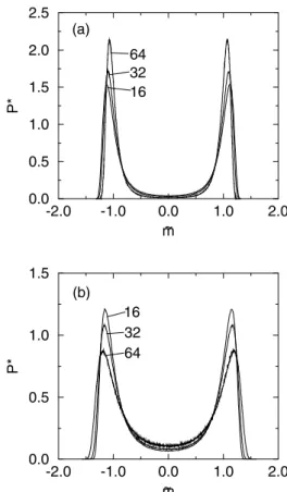
Let us first discuss the spin-1/2 Ising model. Fig. 2 shows the distributionP∗ as a function of the normalized
magnetizationm˜ for temperatures different from the critical valueTc. As expected, one can see that for a temperature lower thanTc(Fig. 2a), the maximum value ofP∗increases
when the lattice sizeL increases, while for a temperature greater thanTc, an increase ofLleads to a decrease of the corresponding peaks ofP∗(see Fig. 2b).
In other words, suppose we have a distribution function P∗( ˜m) for a given L (say for example,
L = 16) at a fixed temperature TL=16. IfTL=16 < Tc, a similar distribution will be obtained for a bigger lattice (e.g.,L = 64) at a different temperatureTL=64 such that
TL=16< TL=64< Tc. Analogously, ifTL=16> Tc, we
-2.0 -1.0 0.0 1.0 2.0
m 0.0
0.5 1.0 1.5
P*
-2.0 -1.0 0.0 1.0 2.0
m 0.0
0.5 1.0 1.5 2.0 2.5
P*
16 32 64 64 32 16
~
~ (a)
(b)
Figure 2. Scaling functionP∗( ˜m)for the spin-1/2 Ising model withL= 16, 32, and 64 at a fixed temperatureT: (a) lower than Tc(T = 2.2472) and (b) greater thanTc(T = 2.2831). The error
bars have been ommited for clarity.
will haveTL=16> TL=64> Tc. This fact suggests a mech-anism to obtain the critical temperature, as well as the ex-ponentν and the universal distribution, for the system un-der study. Table I shows the temperatures of several lattice sizes we have used to obtain the distributions displayed in Fig. 3. These temperatures were evaluated as follows. For
L = 64and a given temperature, for instanceT = 2.2989
in Table I, we compute the corresponding probability dis-tribution of the order parameter, which will be the “refer-ence” distribution. For other values ofL, we search for the temperatureTLwhich gives a distribution equivalent to the reference one. In this way, we obtain the data shown in the second column of Table I. Taking a different reference dis-tribution, obtained at a different temperature forL= 64, we have another set ofTL, and so on. All the distributions so obtained are depicted in Fig. 3. It means that each curve in Fig. 3 is in fact a superposition of six different distributions taking at the temperatures given in Table I.
Since one expects that the difference|TL−Tc|scales as
L−1/ν, whereνis the correlation length critical exponent, a
finite-size scaling analysis can be done to estimate the criti-cal values of the infinite system. In Fig. 4a, we have a plot ofTL vs. L−1/ν, withν = 1, using the values of the first
five columns of Table I, which confirms the exact exponent
TABLE I. Temperature for different lattice sizes at which the distributionP∗( ˜m)forL= 16
−48is the same as that obtained forL= 64
at the shown temperatures (spin-1/2). Error in parentheses affects the last digits. The second and third columns correspond to temperatures greater than the critical one, and the two following columns correspond to temperatures lower than the critical one. The last column represents the data whenP∗( ˜m)forL= 64is obtained atT
c.
Size Temperature (in units ofJ/kB)
16 2.3923(11) 2.3272(8) 2.2477(8) 2.1901(10) 2.27221(52) 20 2.3666(8) 2.3154(8) 2.2502(8) 2.2036(10) 2.27092(52) 24 2.3502(8) 2.3073(5) 2.2528(5) 2.2134(7) 2.27015(52) 32 2.3288(5) 2.2973(5) 2.2563(5) 2.2262(5) 2.26963(26) 48 2.3089(5) 2.2878(5) 2.2604(5) 2.2399(5) 2.26937(26)
64 2.2989 2.2831 2.2624 2.2472 2.269184
-2.0 -1.0 0.0 1.0 2.0
m 0.0
0.5 1.0 1.5 2.0 2.5
P*
~
T < Tc
T Tc
T > Tc
≅
Figure 3. Normalized distributionP∗( ˜m)for systems with lattice sizes and temperatures shown in Table I. Each curve is a supper-position of six different distributions taking with the data from this table.
In this case (very close toTc, last column of Table I), however, it is known that |TL −Tc| scales asL−(1+θ)/ν,
whereθis the correction to scaling exponent [1]. In Fig. 4b, we plot the estimatesTL as a function of L−(1+θ)/ν with
ν = 1 and θ = 2 [14]. Linear regression gives Tc = 2.2693(1)for the infinite system, which is in fact quite close to the exact one.
In order to measure the applicability of the present mechanism for obtaining the transition temperature from non-universal distributions, we also study the spin-1 Ising model. To have an idea of the value of Tc, one just per-forms short simulations in a range of temperatures to check whether the probability distributionP(m)has single or dou-ble peak. Then, one proceeds according to the same manner already discussed for the spin-1/2 case. We fix the temper-ature and verify how the peaks of the distribution change if the lattice size L increases. Fig. 5 shows the distribu-tions obtained for lattice sizes L = 12, 16, 24, and 32 at two different temperatures: T = 1.660andT = 1.720. In the former case an increasing lattice size leads to increasing peaks, while in the latter case the height of the peaks de-creases when the lattice becomes larger. Thus, we conclude that the transition temperature is between 1.660 and 1.720, and hence we perform longer simulations in this temperature range.
0.00000 0.00010 0.00020 L-(θ+1)/ν 2.2680
2.2690 2.2700 2.2710 2.2720 2.2730 2.2740
TL
0.01000 0.03000 0.05000 0.07000 L-1/ν
2.1500 2.2500 2.3500 2.4500
TL
Figure 4. (a) TemperatureTLas a function ofL−1/ν withν= 1.
Different symbols correspond to different choices of the reference distribution (from top to bottom we have the results from the sec-ond to fifth columns of Table I). Error bars are smaller than the symbol sizes. (b) TemperatureTLas a function ofL−(1+θ)/νwith
ν= 1andθ= 2taking the data of the last column of Table I.
The procedure now is the same as that we have done for the spin-1/2 model. We fix the temperature and compute
P∗( ˜m)for the lattice withL = 32(reference distribution).
For a differentL, we search for the temperature that gives a distribution equal to the reference one. Table II shows the temperatures so obtained. For each set of temperatures (which corresponds to each column of Table II), we plotTL
vs. L−1/ν and vary the exponentν until we get a straight
line. Thus, each column of Table II gives an independent estimate ofν and also of the critical temperatureTc. Fig. 6 illustrates this procedure. By taking the mean value of these quantities, one obtainsν = 1.0(1)andTc = 1.6933(16), where the latter agrees well with the valueTc= 1.6935(10)
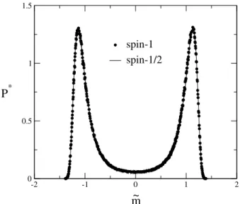
distributionP∗( ˜m). Fig. 7 shows the distribution P∗( ˜m)
on a L = 64 lattice for spin-1/2 and spin-1 models, and confirms the fact that both systems belong to the same uni-versality class, as already expected.
-2 -1 0 1 2
0 0.5 1
-2 -1 0 1 2
0 0.5 1 1.5 2 2.5 3
32 24 16 12
12 16 24 32 (b)
(a)
P
*P
*m
~
Figure 5. Scaling functionP∗( ˜m)for the spin-1 model on square lattices withL= 12,16,24, and 32 at a fixed temperatureT: (a) lower thanTc(T = 1.660) and (b) greater thanTc(T = 1.720).
TABLE II. Temperature for different lattice sizes at which the dis-tributionP∗( ˜m)forL= 12
−24is the same as that obtained for
L = 32at the shown temperatures (spin-1). Error in parentheses affects the last digits. The second and third columns correspond to temperatures greater than the critical one, and the two following columns correspond to temperatures lower than the critical one.
Size Temperature (in units ofJ/kB)
12 1.598(4) 1.652(2) 1.708(2) 1.765(1) 16 1.624(2) 1.664(2) 1.705(2) 1.747(1) 24 1.649(2) 1.675(1) 1.702(1) 1.730(1) 32 1.660(2) 1.680(1) 1.700(1) 1.720(1)
3
Conclusions
The present approach, using just the order parameter distri-bution, seems to be a robust way to obtain the criticality of magnetic systems, regarding its universal and non-universal aspects. There is a clear distinction between the finite-size
0 0.05 0.1
1.55 1.6 1.65 1.7 1.75 1.8
T
LL
-1/νFigure 6. TemperatureTLas a function ofL−1/ν(spin-1).
Differ-ent symbols correspond to differDiffer-ent choices of the reference distri-bution (see Table II). The values ofνthat give the best linear fit were (from top to bottom):ν= 0.9(1),ν= 0.9(1),ν= 1.1(1), andν= 1.1(1). Error bars are smaller than the symbol sizes.
-2 -1 0 1 2
0 0.5 1 1.5
spin-1 spin-1/2
m
~
P
*Figure 7. Universal function P∗( ˜m)for lattice sizeL = 64 at temperatures obtained in this work: T = 2.2693for spin-1/2 and T = 1.6933for spin-1.
behavior ofP∗close to the critical temperature (scaling with
L−(1+θ)/ν) or away from it (scaling with L−1/ν), as
We feel, however, that reweighting the distribution is more easily done for smaller systems. Application of the present procedure to other models (pure and random), as well as to multicritical behavior, will be very welcome; some are now in progress.
Acknowledgments
We would like to thank R. Dickman for fruitful discus-sions and a critical reading of the manuscript. Financial sup-port from the Brazilian agencies CNPq, CAPES, FAPEMIG and CIAM-02 49.0101/03-8 (CNPq) are gratefully acknowl-edged.
References
[1] K. Binder, Z. Phys. B43, 119 (1981).
[2] A.D. Bruce, J. Phys. C14, 3667 (1981).
[3] D. Nicolaides and A.D. Bruce, J. Phys. A21, 233 (1988).
[4] J.A. Plascak and D.P. Landau, Phys. Rev. E67015103 (R) (2003).
[5] M.M. Tsypin and H.W.J. Bl¨ote, Phys. Rev. E62, 73 (2000).
[6] A. D. Bruce and N. B. Wilding, Phys. Rev. Lett. 68, 193 (1992); N. B. Wilding and A. D. Bruce, J. Phys.: Condens. Matter4, 3087 (1992); N. B. Wilding, Phys. Rev. E52, 602 (1995).
[7] K. Rummukainen, M. Tsypin, K. Kajantie, M. Laine, and M. Shaposhnikov, Nucl. Phys. B532, 283 (1998).
[8] C. Alexandrou, A. Borici, A. Feo, P. de Forcrand, A. Galli, F. Jegerlehner, and T. Takaishi, Phys. Rev. D 60, 034 504 (1999).
[9] M.E. Fisher in Critical Phenomena, edited by M.S. Green (Academic, New York, 1971).
[10] J. Adler and I.G. Enting, J. Phys. A17, L275 (1984).
[11] J.A. Plascak, A.M. Ferrenberg, and D. P. Landau, Phys. Rev. E65, 066702 (2002).
[12] R. Dickman and W.C. Schieve, J. Physique45, 1727 (1984).
[13] A.M. Ferrenberg and R.H. Swendsen, Phys. Rev. Lett.61, 2635 (1988).