enrichment and stability in an omnivory system
Faria, LDB.
a* and Costa, MIS.
baSetor de Ecologia, Departamento de Biologia, Universidade Federal de Lavras – UFLA
CEP 37200-000, Lavras, MG, Brazil
bLaboratório Nacional de Computação Científica
Av. Getúlio Vargas, 333, CEP 25651-070, Petrópolis, RJ, Brazil *e-mail: [email protected], [email protected]
Received April 28, 2008 – Accepted July 18, 2008 – Distributed November 30, 2009 (With 6 figures)
Abstract
Food webs usually display an intricate mix of trophic interactions where multiple prey are common. In this context omnivory has been the subject of intensive analysis regarding food web stability and structure. In a three species om-nivory setting it is shown that the modeling of prey preference by the top predator may exert a strong influence on the short as well as on the long term dynamics of the respective food web. Clearly, this has implications concerning the stability and the structure of omnivory systems under disturbances such as nutrient enrichment.
Keywords: omnivory, stability, prey preference, nutrient enrichment.
Interação entre preferência alimentar, enriquecimento de
nutrientes e estabilidade em uma onivoria
Resumo
Redes tróficas apresentam geralmente uma variada rede de interações onde múltiplas presas são comuns. Neste con-texto, a onivoria vem sendo objeto de intensas análises à luz da estabilidade e estrutura do sistema. A modelagem do termo de preferência pelo predador de topo sobre suas presas pode exercer uma forte influência sobre as dinâmicas transiente e de longo prazo em uma rede trófica onívora composta por três espécies. Claramente, isto tem implicações sobre a estrutura e estabilidade do sistema sob distúrbios tais como o enriquecimento por nutrientes.
Palavras-chave: onivoria, estabilidade, preferência alimentar, enriquecimento de nutrientes.
1. Introduction
The behaviour of models with three or more interac-tive species have been investigated by several authors, focusing on how different aspects may affect their dy-namics. Omnivory, defined as the feeding on nonadja-cent trophic levels and found to be widespread in nature (Polis et al., 1989), is a relevant topic of this sort of investigation. It has been studied with respect to condi-tions for coexistence, nutrient enrichment, behavioural, top-down and bottom-up effects (Holt and Polis, 1997; Diehl and Feibel, 2000; Hart, 2002; Kuijper et al., 2003), amongst others.
In a study to re-evaluate the omnivory-stability rela-tionship in food web dynamics, McCann and Hastings (1997) proposed a three-species omnivory with a fixed preference term, concluding that intermediate omnivory levels (dictated by the preference term) tend to stabilise the food web dynamics. This type of selection term has been utilised in several works dealing with food web dy-namics. However, the investigation of alternative forms
of preference modeling has been called for so as to assess their influence on the results of food web theory (Huxel and McCann, 1998; Jefferies, 2000).
dP dt x y
wR
R w C wRP x y
w C
C wR w CP x P
p pr p pc p
=
+ − + +
−
+ + − −
02 1 0
1 1
( )
( )
( )
Resorting to the formulation of preference put for-ward by Post et al. (2000), the omnivory model (1), (hereinafter named switching model (SW)), is proposed here:
dR dt R
R
K x y
R
R RC
wR
wR w Cx y
R
R RP
c c p pr
= −
1 − 0+ − + −(1 ) 02+
dC
dt x y
R
R RC
w C
wR w Cx y
C
C CP x C
c c p pc c
= + − − + − + − 0 0 1 1 ( )
( ) (3)
dP dt
wR wR w Cx y
R R RP
w C wR w Cx y
C C CP x
p pr p pc p
= + − + + + −− + − ( ) ( ) ( ) 1 1 1 02 0 P P
The terms switching and non-switching presented above are used to characterise the preference structure, besides distinguishing between the two models to be analysed. The precise interpretation of the preference pa-rameter p is different in these two models: in model (2) it represents the fraction of actual searching time (i.e., not counting handling time) allocated to searching for prey of species 2, whereas in model (3) it represents a weigh-ing factor such that the fraction of the total time spent searching for plus the handling of either prey species is proportional to their weighed frequency in the popula-tion, with p being the weighing factor for species 2 and 1-p for species 1. Further, for 0 < p < 0, model 2 depicts a functional response multi-species type II (Hassel, 1978), and model 3 depicts a functional response type III which gives to the model a capacity to switch between func-tional response type II (e.g., p = 0 and 1) and funcfunc-tional response type III (e.g., 0 < p < 0).
The dynamics of NSW (2) and SW (3) will be ana-lysed with respect to preference term w. The analysis will span the whole range of preference, i.e., 0 ≤ w ≤1, where for w = 0 the omnivory model (2) becomes a tri-trophic food chain (see Hastings and Powell, 1991 for more information), while for w = 1 it becomes a food web with two consumers sharing a common resource (competition) - two of the omnivory background struc-tures according to Vandermeer (2006). This range gives a complete picture of the dynamical effects of preference modeling when the system’s structure gradually changes between these extremes.
Both models will also be analysed with respect to a gradient of the basal productivity K. The impor-tance of analysing the influence of primary productiv-ity (i.e., bottom-up effect) lies in the fact that, among others, the habitat destruction and/or fragmentation rate by anthropogenic activities is continuously increasing. Furthermore, in theoretical ecology some endeavor has been directed to understand the influence of the carrying capacity level on the structure of food webs, since it may destabilise food web dynamics (e.g., paradox of enrich-ment, Rosenzweig (1971)), (Abrams & Roth, 1994).
These bifurcation diagrams were developed using FORTRAN 95. The local minima and maxima long-is more prone to predation as its density increases with
respect to other alternative prey.
In this light, a switching preference function is intro-duced in the omnivory model presented in McCann and Hastings (1997) so as to evaluate whether such structural change could lead to major dynamical modification with respect to the preference modeling. In addition, regarding nutrient enrichment, an analysis is performed for these two types of preference. Results evidence that there may be significant alteration in dynamical behaviour, stress-ing thus, the importance of preference modelstress-ing in food web theory.
2. Methods
2.1. Omnivory models
The omnivory model is characterised by a logistic growth of the resource population (R), functional re-sponse type II of the consumer (C) on resource and pred-ator (P) on resource and consumer. A model for a three species omnivory food web (a closed loop omnivory according to Vandermeer, 2006) can take the following form:
dR dt R
R
K x y
R
R RC x y R
R RP
c c p pr
= − −
+ − +
1
0 02
dC dt x y
R
R RC x y C
C CP x C
c c p pc c
=
+ − + −
0 0
(1)
dP dt x y
R
R RP x y C
C CP x P
p pr p pc p
=
+ + + −
02 0
where R, C and P are resource, consumer and predator densities, respectively; K is the resource carrying capaci-ty; R0, R02 are the half-saturation densities of the resource (R) and C0 the half-saturation density of the consumer (C); xc, xp are the mass-specific metabolic rates of con-sumer and predator species, respectively; yc, ypr and ypc are measures of ingestion rate of consumer species and predator (Yodzis and Innes, 1992; McCann and Yodzis, 1994a, b; McCann and Hastings, 1997). Assuming mod-el 1 as framework (see Yodzis and Innes, 1992; McCann and Yodzis, 1994a, b for more details about numerical analyses), model 2 and 3 will be built in two different ways of preference parameters as shown below.
McCann and Hastings (1997) have investigated the omnivory intensity role in the dynamics of the food chain model (1) by adding a non-switching selection term w to the predator functional and numerical response type II as shown in model (2) (hereinafter named non-switching model (NSW)):
dR
dt R
R
K x y
R
R RC x y
wR
R w C wRP
c c p pr
= 1− − + − + − +
1
0 02 ( )
dC
dt x y
R
R RC x y
w C
C wR w CP x C
c c p pc c
= + − − + + − − 0 0 1 1 ( )
w in NSW and SW, respectively. The parameter set em-ployed (xc = 0.40, xp = 0.08, yc = 2.009, ypr = 2.000, ypc = 5.0, R0 = 0.16129, R02 = 0.50 and C0 = 0.50) produces chaotic dynamics in a three species food chain (McCann and Yodzis, 1994a). The results for SW are:
1. SW dynamics becomes a two point cycle for 0 < w < 0.02; for 0.02 < w < 0.77, this cycle dynamics turns into a stable dynamics; it turns back into cycling dynamics for w > 0.77.
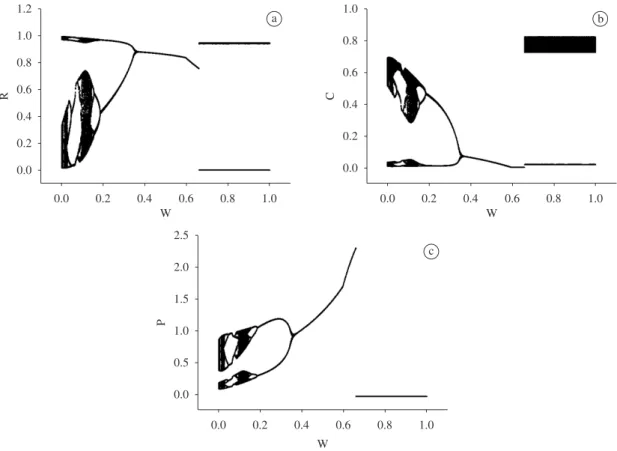
2. On the other hand, in NSW the chaotic dynamic can persist for relatively higher values of the selection term (w < 0.15). The stable dynamics range for NSW (0.35 < w < 0.65) is shorter than the stable dynamics range for the SW (0.02 < w < 0.77). 3. For 0.6 < w < 0.65 consumer extinction occurs
in NSW, while in SW consumer persists for all values of w.
4. In NSW the predator goes to extinction for w > 0.65, while the same happens in the SW only for w > 0.97, increasing thus the range of coexistence of the IGP food web.
Here, the NSW model analysis depicts the whole range of the bifurcation diagram, including the complete value of p (0-1) and the local maxima and minima of the attractor, as opposed to McCann and Hastings (1997) where only local minima was shown and discussed. In term dynamics (solid points) and local minima transient
(dashed line) were obtained for the parameter of prey preference (0 ≤ w ≤ 1) and carrying capacity (0 ≤ K ≤ 2) in a STEP SIZE of 0.001 and ISTEP of 10000. The long-term data simulations were carried out after 5,000 time units, eliminating the transient effect, and the transient data simulations were carried out gathering only the first 5,000 time units.
3. Results
The parameter values taken from the background structures consist of chaotic solutions to the tritrophic food chain (modified by McCann and Yodzis, 1994a, which were also employed by McCann and Hastings, 1997) and unstable solutions (two-point limit cycles and top predator extinction to the competition setting). Two bifurcation diagrams for each population as a function of the selection term w and the primary productivity (K) were built for the NSW and SW models, in order to in-vestigate the interplay among omnivory, preference and basal productivity.
3.1. Prey preference
Figures 1 a-c and 2 a-c depict the local maxima and minima long-term (solid points), and the local minima transient (dashed line) dynamic for a range of preference
a b
c
spectrum between the tritrophic food chain and competi-tion setting for NSW and SW models:
• w=0.11-predatorpreferenceontheconsumeras its food intake. This case corresponds to chaotic dynamics in NSW.
• w=0.5-maximumdegreeofomnivory.
• w=0.89-predatorpreferenceontheresourceas its food intake. This case corresponds to a mirror image of w = 0.11.
this way, this study expands the numerical results of model 2 and compares them with the results of model 3.
To sum up, and comparing with NSW in McCann and Hastings (1997), the long-term analysis shows that SW is able to stabilise the omnivory food web for lower values of w by placing the population minima further away from the axes.
3.2. Gradient of productivity (enrichment)
3.2.2. Long Term Dynamics (attractors)
Throughout the productivity gradient the preference term w was chosen to take on three values along the
a
b
c
a
b
c
Figure 2. Bifurcation diagram for SW for 0 ≤ w ≤1. The solid points give the local maxima and minima for the at-tractor. a: resource (R); b: consumer (C); c: predator (P). Parameter values are the same as in Figure 1.
A striking difference is the coexistence of all three species along the nutrient gradient in SW, as opposed to consumer extinction in NSW.
When preference is directed towards the resource (w = 0.89), the bifurcation analysis of NSW and SW suggest quite similar dynamical behaviour for the re-source and the consumer. The same applies to the K range of stability and instability. The results are as fol-lows.
1. Only the resource is able to invade and persist for 0 < K ≤ 0.16.
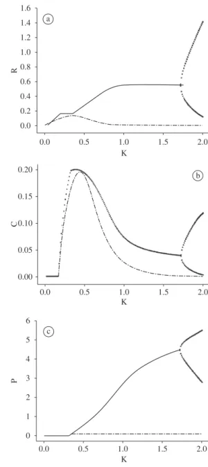
Figure 3a-c depicts the long-term local maxima and minima (solid points), and the transient dynamics local minima (dashed line) in NSW for a range of carrying capacities above and below that given in the standard model (1), where K = 1.
For w = 0.11 the dynamical results of NSW can be summarised as follows:
1. For 0 < K ≤ 0.16, only the resource can invade and persist.
2. Resource and consumer can persist in a stable state for 0.16 ≤ K < 0.25. Predator is able to invade and persist in a stable state for K ≥ 0.25, keeping the consumer density constant.
3. Two point limit cycle begins to occur for K > 0.58, reaching a chaotic dynamics for 0.82 < K < 1.45. These outcomes point to a dynamical variety as a response to nutrient enrichment for NWS in all three trophic levels.
Figure 4 a-c displays the effects of nutrient enrich-ment on the resource for SW when the predator prefer-ence is on the consumer (w = 0.11). The following points are brought out:
1. Consumer invades and persists for K > 0.16, while predator does the same for K > 0.25; thereafter all three trophic levels coexist in a stable steady state.
2. After predator’s invasion, there is a sharp decrease in the consumer level, while in NSW the consumer level is constant after predator’s invasion. 3. At relatively high carrying capacities (K > 1.66),
SW shows a two point limit cycle.
According to the results, SW showed to be more sta-ble along the carrying capacities values than NSW.
For w = 0.5 Figure 5a-c displays the results for the NSW:
1. Only the resource is able to invade and persist for 0 < K ≤ 0.16.
2. For 0.16 ≤ K ≤ 0.30, resource and consumer coexist in a stable state, where consumer density increases and resource density remains constant. 3. When predator population is able to invade and
persist (K≥ 0.30), the consumer density decreases steadily attaining zero at K = 1.13. Thereafter, the coexistence of predator and resource obeys standard predator-prey models in face of nutrient enrichment (i.e., constant resource and increasing predator level). Coexistence for the three species occurs for 0.30 ≤ K ≤ 1.13.
For w = 0.5 Figure 6a-c displays the results for SW, which are summed up next.
1. The consumer is able to invade and persist for K > 0.16.
2. The predator invades and persists for K > 0.30, when all three trophic levels coexist in a stable state.
3. This stable state ceases to exist for K ≥ 1.7, when a two point limit cycle ensues.
a
b
c
Figure 6. Bifurcation diagram for nutrient enrichment for NSW (w = 0.5). The solid points give the local maxima and minima for the attractor and the dashed line gives the glo-bal minima for the transient phase (first 5,000 time units). a) resource (R); b) consumer (C); c) predator (P). Parameter values are the same as in Figure 1.
a
b
c
Figure 5. Bifurcation diagram for nutrient enrichment for NSW (w = 0.5). The solid points give the local maxima and minima for the attractor and the dashed line gives the glo-bal minima for the transient phase (first 5,000 time units). a) resource (R); b) consumer (C); c) predator (P). Parameter values are the same as in Figure 1.
2. Consumer is able to invade and attains a stable state for 0.48 > K > 0.16.
3. For K > 0.48, both systems exhibit complex behaviour.
4. As to the predator dynamics NSW suggests that its invasion cannot occur for K < 1.77. An unstable coexistence ensues for 1.77 ≤ K < 1.90.
For K > 1.90 the whole system collapses. On the other hand in SW, predator invasion is possible for K > 0.66, leading the food web to a coexistence in complex cycles.
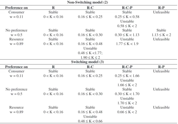
The attractor dynamical results are summed up in Table 1 for NSW and SW regarding coexistence, stabil-ity and productivstabil-ity.
a
b
Table 1. The attractor dynamics with respect to the predator preference for NSW and SW models regarding coexistence, stability and productivity.
Non-Switching model (2)
Preference on R R-C R-C-P R-P
Consumer w = 0.11
Stable 0 < K < 0.16
Stable 0.16 ≤ K < 0.25
Stable 0.25 ≤ K < 0.58
Unstable 0.58 ≤ K < 2
Unfeasible
No preference w = 0.5
Stable 0 < K < 0.16
Stable 0.16 ≤ K < 0.30
Stable 0.30 ≤ K < 1.13
Stable 1.13 ≤ K < 2 Resource
w = 0.89
Stable 0 < K < 0.16
Stable 0.16 ≤ K < 0.48
Unstable 0.48 ≤ K <1.77;
1.90 ≤ K ≤ 2
Unstable 1.77 ≤ K < 1.9
Unfeasible
Switching model (3)
Preference on R R-C R-C-P R-P
Consumer w = 0.11
Stable 0 < K < 0.16
Stable 0.16 ≤ K < 0.25
Stable 0.25 ≤ K < 1.66
Unstable 1.66 ≤ K < 2
Unfeasible
No preference w = 0.5
Stable 0 < K < 0.16
Stable 0.16 ≤ K < 0.30
Stable 0.30 ≤ K < 1.70
Unstable 1.70 ≤ K < 2
Unfeasible
Resource w = 0.89
Stable 0 < K < 0.16
Stable 0.16 ≤ K < 0.48
Unstable 0.48 ≤ K < 0.66
Unstable 0.66 ≤ K < 2
Unfeasible
3.3. Transient dynamics
With respect to the chosen preference degrees along a productivity gradient, the local transient minima simula-tions suggest similar behaviours for both NSW and SW despite the quite markedly different dynamical behaviours in the long term. The dashed lines of Figures 3a-c, 4a-c, 5a-c and 6a-c show that for low K, resource and consumer transient minima remain further from zero and close to their respective attractors, while the predator minima densities remains constant through the whole K values. For a carry-ing capacity with intermediate and high values (K > 0.5) re-source and consumer local transient minima approach zero. Furthermore, irrespective of the model type, the consumer local transient minima seem to follow the attractor through the carrying capacity values, and as result, the transient and attractor dynamics are closer, compared with the same items in the resource and predator population.
4. Discussion
Several works deal with coexistence in food webs as a function of adaptive consumption (Krivan and Diehl, 2005), gradient of omnivory (Vandermeer, 2006), and in a broader context, the degree of poliphagy (Vandermeer and Pascual, 2006). Within this context, omnivory mod-els have been the subject of theoretical investigation as regards the stability and the structure of food webs. Since
in a three species omnivory model the top predator feeds upon the consumer as well as on the resource, the respec-tive models usually resort to employing preference or not in the predation process. When preference is taken into account, it is commonly assumed to be of fixed type (but see Kuijper et al., 2003).
However, as pointed out in Jefferies (2000), Huxel and McCann (1998), an alternative modeling of prey selection, e.g., switching preference (sensu Post et al., 2000), may strongly alter not only the short but the food web long term dynamics as well, when compared with fixed preference. The functional response type II is employed in this analysis based on the fact that several works assert that this kind of functional response is com-monly observed in nature (Hassell, 1978; Faria et al., 2004a,b; Rocha and Redaelli, 2004).
In this view, this work performed an analysis for the purpose of evaluating the influence that fixed and switch-ing preference linked to the functional response type II might exert on the short and long term dynamics of an omnivory food web subject to nutrient and preference degree gradients.
As to nutrient enrichment, for a low preference value (i.e., predator preference on consumer), NSW exhibits complex behaviour for a considerably wide range of K, whereas SW is stable, presenting limit cycles only for high values within the examined K range. For maximum omnivory (w = 0.5), NSW presents stability all over the carrying capacity range. However, coexistence is only possible up to a critical value of K, above which con-sumer goes to extinction. On the other hand, SW predicts a stable coexistence, with two point limit cycles only for high K. For a high preference value (i.e., predator prefer-ence on resource), both models produce a wide range of instability and the coexistence of all three trophic levels is possible solely in an unstable state in SW. Despite the dynamical outcomes having significant differences, both models evidence instability with respect to increasing carrying capacity as predicted by the paradox of enrich-ment (Roseinzweig, 1971).
Regarding transient dynamics and nutrient gradient, resource and consumer transient minima remain further from zero and close to their respective attractors for low levels of carrying capacity, while the predator minima densities remain constant through the whole K values. Furthermore, for a carrying capacity with intermediate and high values (K > 0.5) resource and consumer local transient minima approach zero. Irrespective of the mod-els, consumer local transient minima seem to follow the attractor through the carrying capacity gradient.
The transient results obtained here may be of impor-tance as to empirical settings, since those are usually per-formed over a relatively short time scale. Diehl and Feibel (2000) carried out an experiment generating a time series of an intraguild food web (e.g. two ciliates and one bac-terium) which suggested that coexistence of both ciliates may be affected by the transient dynamics. Moreover, their experiment showed that for low enrichment levels the consumer transient approached the attractor, while higher levels of enrichment pushed the transient dynam-ics away from the attractor’s (see Figure 5a, p. 209 in Diehl and Feibel, 2000). Such results are theoretically corroborated by the non preference setup of SW (with maximum omnivory, w = 0.5). Although it is not possi-ble to perform a direct comparison with the experimental setting due to the arbitrary values used in this analysis, the results suggest that low values of carrying capacity values may produce more stable consumer dynamics, thus enabling a recovery from low densities up to the attractor.
The bifurcation analysis of the presented determin-istic models partially embeds the intrinsic uncertainty of the model parameters, since it displays the possible dy-namical behaviours as a function of some of the analysed parameters values ranges. As a matter of fact, other math-ematical modeling structures, such as probabilistic mod-els and/or stochastic differential equations could handle as well the aforementioned parameter uncertainties.
The results shown here point out the importance of preference modeling in the determination of long as well
as short term food web dynamics. It is therefore sug-gested that dynamical analysis of systems where multi-ple prey are present should consider alternative ways of preference modeling. This is certainly the case of most natural food webs where an intricate mix of trophic in-teractions usually occurs.
References
ABRAMS, PA. and ROTH, D., 1994. The effects of enrichment of three species food chain with nonlinear functional responses. Ecology, vol. 75, no. 4, p. 1118-1130.
DIEHL, S. and FEIBEL, M., 2000. Effects of enrichment on three-level food chains with omnivory. American Naturalist, vol. 155, no. 2, p. 200-218.
FARIA, LDB., GODOY, WAC. and TRINCA, LA., 2004a. Dynamics of handling time and, functional response by larvae of Chrysomya albiceps (Dipt., Calliphoridae) on different prey species. Journal of Applied Entomology, vol. 128, no. 6, p. 432-436
FARIA, LDB., TRINCA, LA. and GODOY, WAC., 2004b. Cannibalistic behavior and functional response in Chrysomya albiceps (Diptera: Calliphoridae). Journal of Insect Behavior, vol. 17, no. 2,p. 251-261.
HART, D., 2002. Intraguild predation, invertebrate predators, and trophic cascades in lake food webs. Journal of Theoretical Biology, vol. 218, no. 1, p. 111-128.
HASTINGS, A. and POWELL, T., 1991. Chaos in a three-species food chain. Ecology, vol. 72, no. 3, p. 896-903. HASSELL, MP., 1978. The dynamics of arthropod predator: prey systems. Princeton: Princeton University Press. p. 237.
HOLT, R.D., 1983. Optimal foraging and the form of predator isocline. Am. Nat. vol. 122, 521-541.
HOLT, RD. and POLIS, GA., 1997. A theoretical framework for intraguild predation. American Naturalist, vol. 149, no. 4, p. 745-764.
HUXEL, GR. and McCANN, K., 1998. Food web stability: the influence of trophic flows across habitats. American Naturalist, vol. 152, no. 3, p. 460-469.
JEFFERIES, RL., 2002. Allochthonous inputs:integrating population changes and food web dynamics. Trends in Ecology and Evolotion, vol. 15, no. 1, p. 19-22.
KRIVAN, V. and DIEHL, S., 2005. Adaptive omnivory and species coexistence in tri-trophic food webs. Theoretical Population Biology, vol. 67, no. 2, p. 85-99.
KUIJPER, LDJ., KOOI, BW., ZONNEVELD, C. and KOOIJMAN, SALM., 2003. Omnivory and food web dynamics. Ecological Modelling, vol. 163, no. 1-2, p. 19-32.
MATSUDA, H., KAWASAKI, K., SHIGESADA, N., TERAMOTO, E., RICCIARDI, L.M., 1986. Switching effect on the stability of the prey-predator system with three trophic levels. J. Theor. Biol. 122, 251-262.
McCANN, K. and YODZIS, P., 1994a. Biological conditions for chaos in a three-species food chain. Ecology, vol. 75, no. 2, p. 561-564.
______, 1994b. Nonlinear dynamics and population disappearance. American Naturalist, vol. 144, no. 5, p. 873-879.
MURDOCH, W. W., 1969 Switching in General Predators: Experiments on Predator Specificity and Stability of Prey Populations. Ecol. Mono. 39, 335 354
POLIS, GA., MYERS, CA. and HOLT, RD., 1989. The ecology and evolution of intraguild predation: potential competitors that eat each other. Annual Review of Ecology Systematics, vol. 20, p. 297-330.
POST, MD., CONNERS, ME. and GOLDBERG, DS., 2000. Prey preference by a top predator and the stability of linked food chains. Ecology, vol. 81, no. 1, p. 8-14.
ROCHA, L. and REDAELLI, LR., 2004. Functional response of Cosmoclopius nigroannulatus (Hem.: Reduviidae) to different densities of Spartocera dentiventris (Hem.: Coreidae) nymphae. Revista Brasileira de Biologia = Brazilian Journal Biology, vol. 64, no. 2, p. 309-316.
ROSENZWEIG, ML., 1971. Paradox of enrichment: destabilization of exploitation ecosystems in ecological time. Science, vol. 171, no. 3969, p. 385-387.
VANDERMEER, J., 2006. Omnivory and the stability of food webs. Journal of Theoretical Biology, vol. 238, no. 3, p. 497-504.
VANDERMEER, J. and PASCUAL, M., 2006. Competitive coexistence through intermediate polyphagy. Ecological Complexity, vol. 3, no. 1, p. 37-43.