ABSTRACT: The search for tools to perform soil surveying faster and cheaper has led to the development of technological innovations such as remote sensing (RS) and the so-called spectral libraries in recent years. However, there are no studies which collate all the RS background to demonstrate how to use this technology for soil classification. The present study aims to de-scribe a simple method of how to classify soils by the morphology of spectra associated with a quantitative view (400-2,500 nm). For this, we constructed three spectral libraries: (i) one for quantitative model performance; (ii) a second to function as the spectral patterns; and (iii) a third to serve as a validation stage. All samples had their chemical and granulometric attributes de-termined by laboratory analysis and prediction models were created based on soil spectra. The system is based on seven steps summarized as follows: i) interpretation of the spectral curve intensity; ii) observation of the general shape of curves; iii) evaluation of absorption features; iv) comparison of spectral curves between the same profile horizons; v) quantification of soil attributes by spectral library models; vi) comparison of a pre-existent spectral library with un-known profile spectra; vii) most probable soil classification. A soil cannot be classified from one spectral curve alone. The behavior between the horizons of a profile, however, was correlated with its classification. In fact, the validation showed 85 % accuracy between the Morphological Interpretation of Reflectance Spectrum (MIRS) method and the traditional classification, showing the importance and potential of a combination of descriptive and quantitative evaluations. Keywords: remote sensing, visible and near infrared, spectroscopy, spectral description, spectrum classification
Introduction
The importance of soils is global. The need for food, a better life and environmental quality are factors that suggest all communities should take a close look at soils. To identify the importance of soils in agriculture, soil maps can be used which show their spatial variation. All types of land use planning need a soil map. Undoubtedly, they require hard work and are time consuming. Thus, the need for faster and cheaper soil mapping methods has led the scientific community to search for technological innovations, and an essential prerequisite to soil mapping is soil classification.
Remote sensing for soil classification has been studied since Stoner and Baumgardner (1981) applied this to American soils. Despite the great number of techniques that have led to an improvement in soil analysis, practical approaches have not emerged. Ben-Dor et al. (2008) highlighted that there is a clear need for fusion between spectroscopy techniques and surveying. Soil classification implies the evaluation of all horizons and has posed certain difficulties. Spectral sensing had a great input with Stoner and Baumgardner (1981). However, they did not show, at that time, how to use the information to achieve classification. With the aim of analyzing spectra by shapes and features, Demattê (2002) identified, much later, the differences between tropical soils, that were subsequently used and ratified in case studies by Vasques et al. (2014),
Soriano-Disla et al. (2014) and Fiorio et al. (2014). But they still did not have a method that integrated quantitative and descriptive analysis.
Although there is a hard descriptive background of spectra, researchers show that the information is dispersed. This makes it difficult for users to determine the importance of this interpretation. Sherman and Waite (1985) for example, stress the differences between goethite and hematite, while Madeira Netto (1996) delineates the shape of gibbsite. Despite the descriptive information as used by Bellinaso et al. (2010), quantitative studies play an important role, together with spectral library patterns, as pointed out by Shepherd and Walsh (2002) and Rizzo et al. (2014). But still, how can a user, with spectra in hand arrive at the classification of a soil? How can the observations be collated and integrated so as to to reach the main goal? There are no reports that focus on this aspect.
The present study aims to construct and describe a detailed method for morphological interpretation of spectra with a look at soil identification and classification. This will give support to the definition of Spectral Pedology, as proposed by Demattê and Terra (2014).
Materials and Methods
We established an interpretation strategy for spectral curves in order to provide the best correlation with soil classification of the spectra for all horizons 1University of São Paulo/ESALQ – Dept. of Soil Science, C.P.
09 − 13418-900 − Piracicaba, SP – Brazil. 2CATI/Secretary of Agriculture of São Paulo State, R. Campos Salles, 507 − 13400-200 − Piracicaba, SP – Brazil. *Corresponding author <jamdemat@usp.br>
Edited by: Silvia del Carmen Imhof
José Alexandre Melo Demattê1*, Henrique Bellinaso2, Danilo Jefferson Romero1, Caio Troula Fongaro1
from the same profile. For this, we propose the MIRS method (Morphological Interpretation of Reflectance Spectrum). The method is based on the premise that the ‘interpretation should be performed by a careful examination of morphological and quantitative information where the convergence of evidence can lead to the probable soil classification, being related to the experience of the interpreter in pedology and remote sensing’.
The system
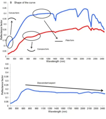
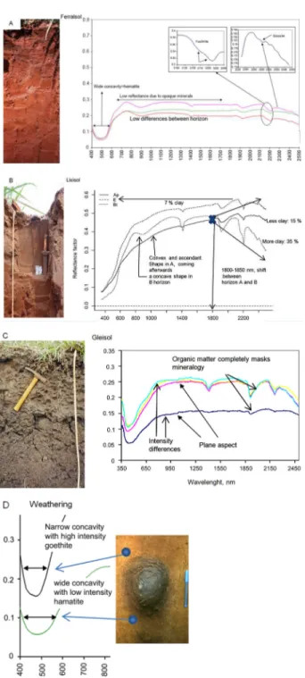
The system is divided into seven steps as follows. The first step refers to the interpretation of the intensity of the spectral curve (Figure 1A). The second step is to observe the general shape of the curves along the complete spectrum (Figure 1B), such as ascendant, descendant or plane (Figure 1C). It is possible that a spectral curve has an ascendant aspect in a particular wavelength and then changes to plane or even descendant in another wavelength (Figure 1D). The third step consists of the evaluation of absorption features, usually promoted by mineralogy in specific wavelengths (Figure 1E); and are described in the literature (i.e., hematite, goethite, gibbsite, kaolinite, montmorilonite, water, organic matter and others).
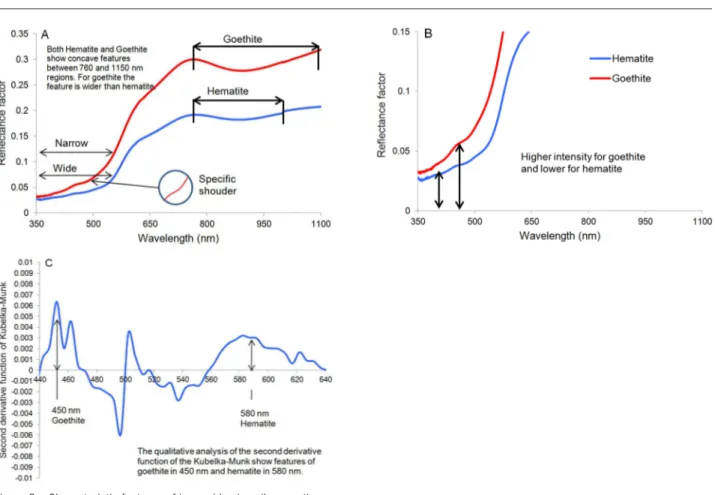
The fourth step is the comparison of spectral curves between horizons in the same profile. One soil may present distinct spectral curves for each horizon while another may present similar spectral curves in the same profile (Figure 1F). Figures 2 and 3 show the main characteristic features of minerals likely to be observed in a spectral curve.
The fifth step is based on a quantitative view of the spectral data. The user needs to prepare a spectral library with many samples to construct models which can quantify certain soil attributes such as cation exchange capacity (CEC), clay, organic matter and iron. In the present study we constructed this database with samples from Brazilian regions, with a total of 7,185 soil samples. The organic carbon (Corg), organic matter (OM) (g kg−1), P (mg kg−1), K, Ca, Mg, Al, H+Al (mmol
c kg −1),
the calculations of the Sum of Cations (SB), CEC, base saturation (V %), and aluminum saturation (m %) (Raij et al., 2001) were determined for all samples. Proportions of sand, and clay were also determined (Camargo et al., 1986). Furthermore, the pH (in H2O and KCl), and Fe2O3, TiO2, MnO, Si2O4 and Al2O3 contents resulting from sulfuric acid digestion were calculated (Camargo et al., 1986). The clay fraction activity, Ki and Kr rates, were also calculated.
The color of dry samples was obtained from a chrometer using the Munsell color system. Since the color is determined from dry, not wet, samples and the chrometer determines hues in more detail than the conventional Munsell chromaticity diagram, the classification of soils was as follows: red soils were those with hues 2.5YR or redder, yellowish-red soils had hues 2.5YR to 7.5YR, and yellow soils had hues 7.5YR or
even more yellow. Spectral data were obtained in the laboratory with the FieldSpec Pro spectro-radiometer that has a spectral resolution of 1 nm for wavelengths from 350 to 1,100 nm and 2 nm for wavelengths from 1,100 to 2,500 nm. For the collection of reflectance data, the samples were dried at 45 oC for 24 h. After drying,
they were ground and sieved through 2-mm mesh. The reflectance of each sample was given by the average of 100 readings from the sensor. The light collector was placed in a vertical position 8 cm from the sample. The source of light was a 50 W halogen light bulb. As a reference pattern, an espectralon white plate was used and considered to be the 100 % reflectance standard. Besides the spectral reflectance graphs, and in order to complement the identification of features, data were drawn from the second derivative of the Kubelka-Munk function (Scheinost et al., 1998; Sellitto et al., 2009). Using the Unscrambler 9.7 program we generated the models to quantify the soil attributes.
The sixth step is related to a comparison between unknown profile spectra with an already known databank. Again, the user needs to have a spectral library. But in this case, the spectral library is from complete profiles and spectra of horizons, and has to be classified traditionally. This step requires the user to compare the unknown profile with the known profile spectra in a careful investigation as stated in the previous steps. In our study we had 233 soil profiles described morphologically and classified traditionally, with the respective spectra. All profiles were evaluated and described morphologically (Lemos and Santos, 2013). Afterwards, they were classified up to the 3rd category
level of the Brazilian System of Soil Classification (EMBRAPA, 2013) and 2nd category on the World
Reference Base for soil resources (FAO, 2006).
The seventh step is to, finally, collate all morphological and quantitative information, and observe the convergence of evidence which enables the most probable classification for the soil to be reached. The success of this method is related to the user’s experience in pedology and if mostly with spectroscopy.
Validation stage: The spectral data of 13 unknown profiles was inserted into these steps to reach their classification. Soil samples were collected from very different sites in the cities of Araraquara (3); Piracicaba (4); Andradina (1) and Ipaussu (1), i.e., São Paulo State; Três Lagoas (3), State of Minas Gerais, and Maracajú (1), State of Mato Grosso do Sul, all in Brazil. The horizons of each profile were represented by letters in alphabetical order and generically called layers. For example, a profile containing horizons A, E, Bt and C would be labeled A, B, C and D, respectively. In the discussion, when referring to the spectral curve of the Bt horizon, it was referred to as layer C curve. Models to allow the determination of sand (g kg−1), clay (g kg−1), cation exchange capacity
(CEC) (mmolc dm−3), V %, m %, aluminum (Al3+) (mmol c
dm−3), Fe
2O3 (g kg
−1) and TiO 2 (g kg
−1) levels were
by descriptive evaluation and inserted in the databases, observing the performance of the method, as compared with the traditional classification.
Comparison with other systems
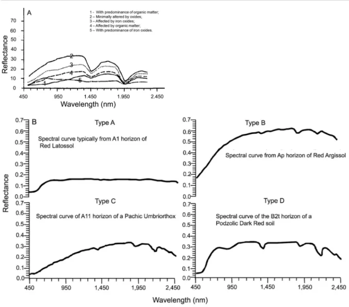
The results were also compared with studies from the literature such as Stoner and Baumgardner (1981) with curves type 1, 2, 3, 4 and 5 and a, b, c
and d from Formaggio et al. (1996) (Figure 4). Stoner and Baumgardner (1981) divide types of curves into the following: 1-with predominance of organic matter, 2-minimally altered by oxides, 3-affected by iron oxides, 4-affected by organic matter, and 5-with predominance of iron oxides; Formaggio et al. (1996) identifies them as follows: a-spectral curves typically from A1 horizon of LR, b-spectral curve from “Ap” horizon of PV, c-spectral
Figure 2 – Characteristic features of soil properties.
curve of A11 horizon of a Pachic Umbriorthox and
d-spectral curve of the Bt2 horizon of a Podzolic Dark Red soil.
Results and Discussion
Thirteen profiles were classified by the MIRS method. Profile 3 shows curves (Figure 5A) of layers A, B and C with average intensity no higher than 0.15, and layer D, which had higher reflectance intensity, though not less than 0.20. The greatest reflectance intensity seen in layer D is explained by the sand content (Table 1). All curves had a descending slope. The curves of lay-ers A, B and C of profile 3 present softened features of kaolinite (2,200 nm) and gibbsite (2,265 nm). In addition, the concave feature is highlighted (850-900 nm), indicat-ing the presence of iron oxides. The curve of layer D did not present a feature typical of gibbsite, but did have features of goethite (450 to 480 nm). The appearance of a goethite feature in layer D matches with the yellowish color of the soil as compared to the other samples (Ta-ble 1). The increase in the amount of goethite promotes more yellowish colors.
The curves of profile 3 were classified as type 5
Figure 3 – Characteristic features of iron oxides in soil properties.
Table 1 – Chemical and granulometrycs profiles analysis.
Profiles1 Horiz. Depth
Granulometry Chemical analysis Color5
Sand Clay CEC4 V m Organic
Matter Al Hue Value Chroma
Ref.2 Pred.3 Ref. Pred. Ref. Pred. Ref. Pred. Ref. Pred. Ref. Pred. Ref. Pred. cm --- g kg−1 --- -- mmol
c kg−1 -- --- % --- --- mg kg−1 --- mmolc kg−1
P03A AP 0-30 150 214 710 729 80.6 58.0 49 38 2 6 33.0 23.7 1.0 1.8 3.9YR 3..5 2.4
P03B BA 30-55 100 158 750 748 55.4 61.2 62 35 0 4 22.0 22.1 0.0 2.6 3.2YR 3.8 2.8
P03C Bi 55-110 130 157 770 735 46.3 48.6 68 33 0 -1 17.0 20.1 0.0 -2.8 3.3YR 3.8 2.5
P03D C 110+ 320 305 430 873 69.1 92.0 12 46 62 11 9.0 22.5 13.0 3.0 7.8YR 4.6 2.8
P04A Ap 0-20 760 701 200 285 35.9 34.1 58 37 5 3 18.0 18.4 1.0 -0.5 6.6YR 4 2
P04B AB 20-45 760 674 200 321 36.0 29.6 44 27 0 8 15.0 16.2 0.0 0.0 6.3YR 4.1 2
P04C BW1 45-80 700 636 260 349 26.7 17.1 51 24 0 5 14.0 14.2 0.0 -5.2 5.8YR 4.3 2.3
P04D BW2 80 670 653 290 331 28.4 13.7 44 22 0 11 12.0 12.9 0.0 -0.4 5.8YR 4.3 2.8
P05A Ap 0-16 130 19 720 842 72.5 66.7 27 15 26 45 23.0 23.4 7.0 10.6 2.9YR 3.5 2.2
P05B Bw1 16-90 140 120 710 861 62.7 68.5 17 20 53 41 18.0 22.5 12.0 10.0 2.7YR 3.5 2.4
P05C Bw2 90-159 90 120 740 774 52.4 39.2 5 9 83 60 18.0 15.4 12.0 6.4 1.9YR 3.6 2.4
P05D Bw3 150+ 110 75 730 804 52.3 48.7 4 25 83 26 13.0 17.1 11.0 6.3 2.0YR 3.5 2.2
P10A Ap 0-30 720 685 120 234 20.4 25.4 51 44 9 24 8.0 9.6 1.0 1.8 9.6YR 5.7 2.5
P10B Bt1 30-60 620 681 220 260 39.4 27.4 75 51 0 13 8.0 9.4 0.0 2.1 8.0YR 5.6 3.9
P10C Bt2 60+ 660 702 180 226 34.3 18.7 88 43 0 27 7.0 6.2 0.0 3.2 8.0YR 5.9 4.1
1P03= Cambissolo Háplico Eutroférrico; text. m. arg.; P04= Latossolo Vermelho-Amarelo Eutrófico; text. média; P05= Latossolo Vermelho Distroférrico; text. m. arg.; álico; P10= Argissolo Amarelo Eutrófico; text. aren/média; A = 0-20 cm; B = 20-40 cm; C = 40-60 cm; D = 60-80 cm; 2Reference determined in laboratory; 3Predicted by spectral models; 4 Cation-Exchange Capacity; 5Determined by colorimeter.
an extremely low reflectance intensity (Madeira Netto and Baptista, 2000). This is in agreement with an Fe2O3 content greater than 200 g kg−1 in this profile (Table 2).
Figure 4 – Spectra of types of curves determined by (A) Stoner and Baungarnder (1981) and (B) Formaggio et al. (1996).
Table 2 – Soil mineralogical analysis.
Sample¹ Depth Fe2O32 TiO22 Ki Kr2 ∆pH2 Clay ativ.2 Minaralogy3
Ref4 Pred5 Ref Pred Ref Pred2 Pred2 Ref Pred Ref Pred Ref Pred Hematite Goethite Gibbsite Kaolinite cm --- % --- mmolc kg−1
P02C 50-115 5.8 14.9 0.58 1.8 1.7 0.9 1.3 1.3 0.5 -0.3 -0.4 97 68 yes yes yes yes
P03C 55-110 24.1 28.5 3.04 3.8 0.9 1.0 1.0 0.6 0.5 -0.2 -0.1 60 41 yes yes yes no
P04C 45-80 4.6 13.9 0.62 1.6 0.7 0.7 1.1 0.5 0.4 -0.1 -0.3 103 97 no yes yes yes
P05C 90-159 0.2 19.3 0.13 2.2 1.3 1.1 1.8 1.2 0.8 -0.9 -0.8 71 32 yes no no no
P06C 40+ 23.7 27.0 2.8 3.4 1.5 1.4 1.6 0.9 0.6 -0.2 -0.1 232 94 yes yes no yes
P07C 70-120 7.1 22.7 0.68 2.2 1.9 1.4 1.7 1.5 0.8 -0.5 -0.3 52 8 yes yes no yes
P08C 50-95 1.5 9.3 0.13 0.9 2.3 2.2 2.5 2.0 1.7 -0.6 -1.4 499 287 no yes no no
P09C 50-80 2.1 9.7 0.19 0.9 2.6 2.5 3.2 2.2 1.9 -0.9 -1.5 990 323 no no no no
P10C 60+ 1.9 9.4 0.16 1.3 1.6 1.3 1.8 1.3 1.0 -0.8 -0.8 191 135 no yes no yes
Figure 5 – Qualitative description of the profiles 3(A) and 4 (B).
intensity agrees with Demattê and Garcia (1999). The intensity behavior of curve D from profile 3 was adjusted
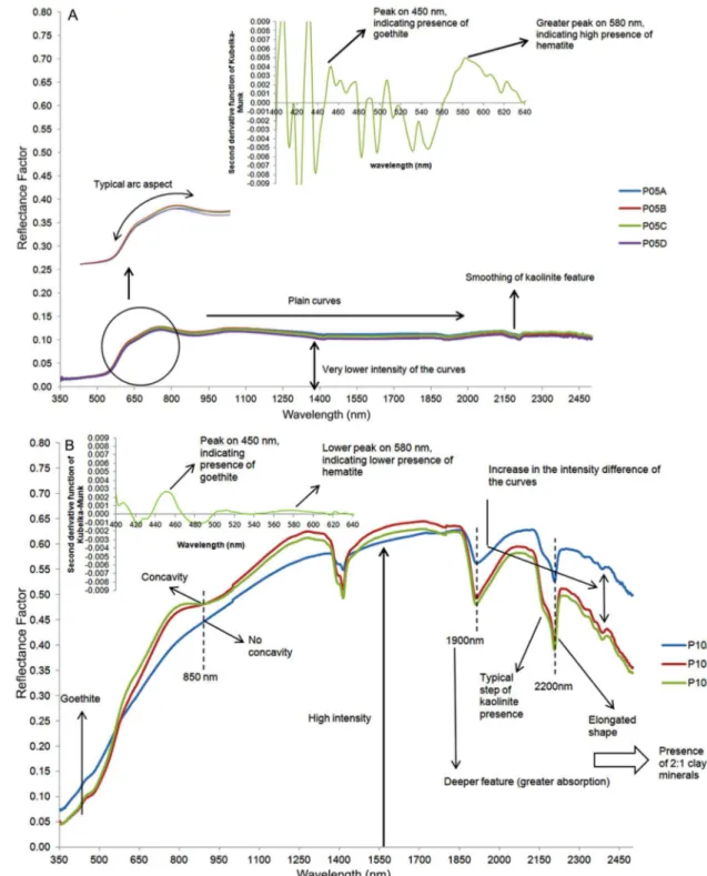
Figure 6 – Qualitative description of the profiles 5 (A) and 10 (B).
Profile 4 (Figure 5B) presented very similar curves between horizons, with reflectance intensities varying between 0.2 and 0.25. This result is expected since results from the determined values of texture and Fe2O3 are high (Tables 1 and 2). With a slope standard slightly ascending. Gibbsite and goethite features were detected. The appearance of the goethite feature matched with
the more yellowish colors found by the colorimetric determination (Table 1). Again, a reduction in the concave feature due to iron oxides (850-900 nm) was observed, promoted by the greater content of O.M.. Based on this evidence, profile 4 was classified as a Ferralsol.
1) confirms the assertion of these authors. However, the Fe2O3 content obtained was low (Table 2), whereas the predicted value matched the authors’ observation, indicating that the predicted result is more reliable than the one given by the reference in this case. Other profiles described in the region (Bellinaso et al., 2010) presented the same spectral characteristics as profile 5, with Fe2O3 content similar to those predicted for this profile. Curves from profile 5 had a standard plane slope, kaolinite and iron oxide features. A characteristic shape between 580 and 850 nm (Figure 6A) was observed in this profile that is usually found in ferric soils.
Figure 6A demonstrates the abundant presence of hematite in profile 5, as calculated by the second derivative of the Kubelka-Munk function. The second derivative for spectral data is able to show the amounts of goethite and hematite present in a particular soil (Sellitto et al., 2009). The greater presence of hematite matches with the colorimetric determination (Table 1), with strongly reddish colors in the soil. All curves from the profiles were classified as type 5 and type a. Thus, profile 5 was classified as a Ferric Dystric – Red Fer-ralsol.
Profile 10 (Figure 6B) presented high albedo curves, with maximum values of 0.6. Although layer A presents a lower clay content than the others (Table 1), the albedo values were close to 1850 nm. Soils with horizons containing more clay developed over argillites or siltites with low iron content, can present albedos similar to those with more sandy horizons (Demattê et al., 2004; Fontes and Carvalho Junior, 2005). However, the greater sand content in layer A, as compared to layers B and C (Table 1), led to a greater intensity in relation to the rest of the measurements starting from 1,850 nm. This standard is characteristic of Lixisols, and agrees with the finding of Demattê (2002).
The curves of profile 10 had an ascending slope. Only the curves in layers B and C presented slope alterations after 1,900 nm. Starting from this spectral layer, the slope was descending (Figure 6B). The second derivative (Figure 6B) demonstrates a greater amount of goethite (450 nm region) in relation to hematite, which is the source of the yellowish color of the soil, confirmed by the colorimetric data, which showed a 8.0YR hue. Fontes and Carvalho Junior (2005) reported that hematite has greater pigmentation power than goethite. Curve A from profile 10 was classified as type 4 and type b and curves B and C as type 2 and type d. As we observed, in the same profile there can be different spectra classifications. Thus, it is not common that a soil class has only one morphological spectral class. This underlines the importance of evaluating the curve of each horizon and afterwards put all together to take a decision.
laboratory analysis were included. While verifying the classifications, the 15 % error was due to differences in classifying profiles 7 and 13 (Table 3). For profile 7, no classification was found when remote sensing techniques were used. However, two possible classes were indicated, and the classification most likely to be correct (Nitisol) matches with the real classification of the profile. The similarity between the spectral characteristics of Ferralsol and Nitisol soils contributes to the error. However, the sharper observation of the gibbsite feature (2265 nm) can be a differentiating factor between the two classes. According to this, the spectral library showed that the gibbsite feature (2265 nm) is sharper in Ferralsols than in Nitisols.
The difference in the classification of Profile 13 was due to different clay contents (Table 1), as was seen when the correct reference data were used. While the reference analysis pointed to a sandy texture for the profile (120 g kg−1), the predicted analysis pointed to 300
g kg−1.
There was a large increase in the number of classification errors in the third level category, where only remote sensing techniques were used (Table 4). This was due to prediction errors related to chemical attributes such as V % and Al3+. The models used for
the prediction of profile attributes have shown low or variable data for the estimation capacity for chemical attributes. The development of regional spectral libraries may contribute to the improvement of chemical attribute predictions, which would increase the efficiency of classifications.
As for the iron characteristic, only profile 1 had a classification difference (Tables 3 and 4). However, this cannot actually be considered as an error, because of the lack of Fe2O3 reference data for this profile. The models used to estimate Fe2O3 have shown an excellent predictive capacity (Nanni and Demattê, 2006). Sellitto et al. (2009) demonstrated how spectroscopy and remote sensing techniques can be accurate in determining iron oxides and Fe2O3. In fact, several authors have indicated a very close correlation between Fe2O3 and reflectance (Brown et al., 2006; Islam et al., 2003; Moron and Cozzolino, 2003).
quantity of iron and clay. When we observe all the hori-zons together, we see few differences between them. In fact, traditional soil classification also does not see dif-ferences between horizons, except the A horizon because of the higher organic matter. When these soils have very
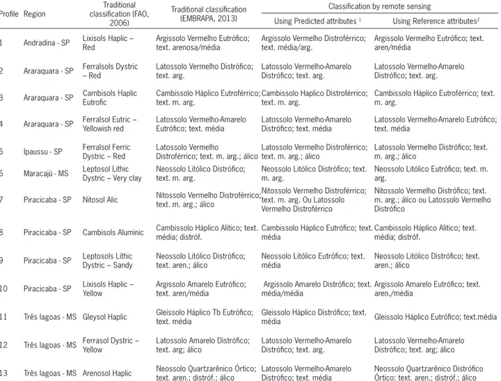
Table 3 – Comparison between real soil classification and the classifications using remote sensing techniques.
Profile Region classification (FAO, Traditional 2006)
Traditional classification (EMBRAPA, 2013)
Classification by remote sensing
Using Predicted attributes 1 Using Reference attributes2
1 Andradina - SP Lixisols Haplic – Red Argissolo Vermelho Eutrófico; text. arenosa/média Argissolo Vermelho Distroférrico; text. média/arg. Argissolo Vermelho Eutrófico; text. aren/média
2 Araraquara - SP Ferralsols Dystric – Red Latossolo Vermelho Distrófico; text. arg. Latossolo Vermelho-Amarelo Distrófico; text. arg. Latossolo Vermelho-Amarelo Distrófico; text. arg.
3 Araraquara - SP Cambisols Haplic Eutrofic Cambissolo Háplico Eutroférrico; text. m. arg. Cambissolo Haplico Distroférrico; text. m. arg. Cambissolo Háplico Eutroférrico; text. m. arg.
4 Araraquara - SP Ferralsol Eutric – Yellowish red Latossolo Vermelho-Amarelo Eutrófico; text. média Latossolo Vermelho-Amarelo Distrófico; text. média Latossolo Vermelho-Amarelo Eutrófico; text. média
5 Ipaussu - SP Ferralsol Ferric Dystric – Red Latossolo Vermelho Distroférrico; text. m. arg.; álico Latossolo Vermelho Distroférrico; text. m. arg.; álico Latossolo Vermelho Distrófico; text. m. arg.; álico
6 Maracajú - MS Leptosol Lithic Dystric – Very clay Neossolo Litólico Distrófico; text. m. arg. Neossolo Litólico Distrófico; text. m. arg. Neossolo Litólico Eutrófico; text. m. arg.
7 Piracicaba - SP Nitosol Alic Nitossolo Vermelho Distroférrico; text. m. arg.; álico Nitossolo Vermelho Distroférrico; text. m. arg. Ou Latossolo Vermelho Distroférrico
Nitossolo Vermelho Distrófico; text. m. arg.; álico ou Latossolo Vermelho Distrófico
8 Piracicaba - SP Cambisols Aluminic Cambissolo Háplico Alítico; text. média; distróf. Cambissolo Háplico Eutrófico; text. média Cambissolo Háplico Alítico; text. média; distróf.
9 Piracicaba - SP Leptosols Lithic Dystric – Sandy Neossolo Litólico Distrófico; text. aren.; álico Neossolo Litólico Eutrófico; text. média Neossolo Litólico Distrófico; text. aren.; álico
10 Piracicaba - SP Lixisols Haplic – Yellow Argissolo Amarelo Eutrófico; text. aren/média Argissolo Amarelo Distrófico; text. média/média Argissolo Amarelo Eutrófico; text. aren./média
11 Três lagoas - MS Gleysol Haplic Gleissolo Háplico Tb Eutrófico; text. média Gleissolo Háplico Distrófico; text.média Gleissolo Háplico Eutrófico; text.média
12 Três lagoas - MS Ferrasol Dystric – Yellow Latossolo Amarelo Distrófico; text. arg; álico Latossolo Vermelho-Amarelo Distrófico; text. arg. Latossolo Vermelho-Amarelo Distrófico; text. arg; álico
13 Três lagoas - MS Arenosol Haplic Neossolo Quartzarênico Órtico; text. aren.; distróf.; álico Latossolo Vermelho-Amarelo Distrófico; text. média Neossolo Quartzarênico Distrófico Órtico; text. aren.; distróf.; álico
1Classification using the qualitative interpretation of the spectral curves predicted by using data and models to estimate; 2Classification using the qualitative interpretation of the spectral curves and data analysis using routine laboratory.
Table 4 – Accuracy rate of classification using remote sensing techniques.
Number of profiles
% agreement for first level category
% agreement for second level
category
% agreement third level category
no % no % no %
Exclusively Using Remote Sensing Techniques (attributes predicted)
13 11 85 11 85 6 46
Using Remote Sensing Techniques and Routine Analysis (reference attributes)
13 12 92 12 92 12 92
high iron content, sometimes even the A horizon cannot be depicted, as observed by Demattê et al. (2004).
Figure 7C shows a Gleysol. This soil presents a high amount of montmorillonite which gives a strong feature at 1900 nm in the B horizon and a specific feature at 2200 nm. The low hematite content is observed by the absence of concavity around 900 nm. Horizon A is hiding the min-eralogy features due to the high organic matter content. Figure 7D shows the descriptive differences between hematite (red color) with a wide concave shape and low
Figure 7 – Spectral curves and features from (A) Ferralsol; (B) Lixisol; (C) Gleisol; and (D) Weathering features.
Although the difference between predicted and ref-erence values is more evident, the classification of soil texture has been shown to be fairly accurate (Table 4). In fact, the quantification of clay has, by and large shown good results (Soriano-Disla et al., 2014), which ratifies its importance in the MIRS system. The prediction errors fit into the variation range of contents for each textural class, leading to good results. The prediction model used for the profile attribute estimates has a good performance regard-ing the quantification of clay and sand also by other au-thors such as Nanni and Demattê (2006). In fact the need for spectral libraries to achieve models for quantification of soil attributes is important for the MIRS system.
The quantitative information gives a different per-spective to the descriptive. It gives a number of the con-tent of the attribute, which reveals punctual information of the sample. On the other hand, the entire spectrum (400-2,500 nm), observed by the perspective of the entire spectrum, reveals the information in its entirety, which includes the combination of all constituents. Thus, the de-scriptive information is absolutely important because it allows the user to ‘see’ the result of this combination and compare it to a known sample. A single number of quanti-fication does not allow this view. Another important con-sideration is the comparison between spectra from all ho-rizons at the same time. Ferralsols show few differences between spectra along horizons, but Lixisols have evident differences. This can be seen from clay quantification. On the other hand, can we see a clay difference in a Red Lixisol (with hematite) when compared to a Yellow Lixi-sol (with goethite)? Yes, by spectra shapes as indicated in this manuscript. Another example is if we have traditional mineralogy information of a soil indicating the presence of gibbsite, can we know the soil class? Yes, if we have the entire spectra, we can detect the feature of gibbsite and
see the color (by shapes showing a presence of hematite or goethite), from the entire shape of the spectra from all ho-rizons and have a preliminary idea of the soil class. This shows the importance and potential of the combination of descriptive and quantitative evaluation of spectra from a profile looking at soil classification.
Conclusions
The individual interpretation of curves does not allow for accurate indication of soil class. The combination of morphological and quantitative remote sensing techniques has proved to be an important tool for classifying soils.
Acknowledgements
The authors thank FAPESP (grant 07/54976-8), for the financial support, CNPq for financial support of the first and third authors, and CAPES for the scholarship of the second author. We also extend thanks to the techni-cal support from Geotechnoliges in Soil Science Group (GeoCis) - http://esalqgeocis.wix.com/geocis.
References
Bellinaso, H.; Demattê, J.A.M.; Romeiro, S.A. 2010. Spectral library and its use in soil classification. Revista Brasileira de Ciência do Solo 34: 861-867.
Ben-Dor, E.; Heller, D.; Chudnovsky, A. 2008. A novel method of classyfing profiles in the field using optical means. Soil Science Society of America Journal 72: 1113-1123.
Brown, D.J.; Shepherd, K.D.; Walsh, M.G.; Mays, M.D.; Reinsch, T.G. 2006. Global soil characterization with VNIR diffuse reflectance spectroscopy. Geoderma 132: 273-290.
Camargo, A.O.; Moniz, A.C.; Jorge, J.A.; Valadares, J.M. 1986. Methods of chemical, physical and mineralogical analysis of soils from IAC = Métodos de análise química, mineralógica e física de solos do IAC. Campinas:IAC (Boletim Técnico, 106) (In Portuguese).
Demattê, J.A.M. 2002. Characterization and discrimination of soils by their reflected electromagnetic energy. Pesquisa Agropecuária Brasileira 37: 1445-1458.
Demattê, J.A.M.; Terra, F.S. 2014. Spectral pedology: a new perspective on evaluation of soils along pedogenetic alterations. Geoderma 217-218: 190-200.
Demattê, J.A.M.; Campos, R.C.; Alves, M.C.; Fiorio, P.R.; Nanni, M.R. 2004. Visible-NIR reflectance: a new approach on soil evaluation. Geoderma 121: 95-112.
Demattê, J.A.M.; Garcia, G.J. 1999. Alteration of soil properties through a weathering sequence as evaluated by spectral reflectance. Soil Science Society of America Journal 63: 327-342.
Empresa Brasileira de Pesquisa Agropecuária [EMBRAPA]. 2013. Brazilian System of Soil Classification = Sistema Brasileiro de Classificação de Solos. 3ed. EMBRAPA, Brasília, DF, Brazil (in Portuguese).
Food and Agriculture Organization [FAO]. 2006. World Reference Base for Soil Resources. FAO, Rome, Italy.
Fiorio, P.R.; Demattê, J.A.M.; Nanni, R.M.; Genú, A.M.; Martins,
J.A. 2014. In situ separation of soil types along transects
employing Vis-NIR sensors: a new view of soil evaluation. Revista Ciência Agronômica 45: 433-442.
Fontes, M.P.F.; Carvalho Junior, I.A. 2005. Color attributes and mineralogical characteristics, evaluated by radiometry, of higly weathered tropical soils. Soil Science Society of America Journal 69: 1162-1172.
Formaggio, A.R.; Epiphânio, J.C.N.; Valeriano, M.M.; Oliveira, J.B. 1996. Spectral behavior (450-2,450 nm) of tropical soils from São Paulo State, Brazil. Revista Brasileira de Ciência do Solo 20: 467-474 (in Portuguese, with abstract in English).
Islam, K.; Singh, B.; McBratney, A.B. 2003. Simultaneous estimation of several soil properties by ultra-violet, visible, and near-infrared reflectance spectroscopy. Australian Journal of Soil Research 41: 1101-1114.
Lemos, R.C.; Santos, R.D. 2013. Manual of Description and Soil Sampling on Field = Manual de Descrição e Coleta de Solo no Campo. Sociedade Brasileira de Ciência do Solo, Viçosa, MG, Brazil (in Portuguese).
Madeira Netto, J.S. 1996. Spectral reflectance of properties of soils. Photointerpretation 34: 59-70.
Madeira Netto, J.S.; Baptista, G.M.M. 2000. Reflectância espectral de solos. Planaltina, Embrapa Cerrados. 55p.
Moron, A.; Cozzolino, D. 2003. The potential of near-infrared reflectance spectroscopy to analyze soil chemical and physical characteristics. Journal of Agricultural Engineering 140: 65-71. Nanni, M.R.; Demattê, J.A.M. 2006. Spectral reflectance
methodology in comparison to traditional soil analysis. Soil Science Society of America Journal 70: 393-407.
Raij, B. van.; Andrade, J.C.; Cantarella, H.; Quaggio, J.A. 2001. Chemical Analysis for Evaluation of Tropicals Soils = Análise Química para Avaliação da Fertilidade de Solos Tropicais. Instituto Agronômico, Campinas, SP, Brazil (in Portuguese). Rizzo, R.; Demattê, J.A.M.; Terra, F.S. 2014. Using numerical
classification of profiles based on Vis-NIR spectra to distinguish soils from the Piracicaba region, Brazil. Revista Brasileira de Ciência do Solo 38: 372-385.
Scheinost, A.C.; Chavernas, A.; Barrón, V.; Torrent, J. 1998. Use and limitations of second-derivative diffuse reflectance spectroscopy in the visible to near-infrared range to identify and quantify Fe oxides in soils. Clays and Clay Minerals 46: 528-536.
Sellitto, V.M.; Fernandes, R.B.A.; Barrón, V.; Colombo, C. 2009. Comparing two different spectroscopic techniques for the characterization of soil iron oxides: diffuse versus bi-directional reflectance. Geoderma 149: 2-9.
Shepherd, K.D.; Walsh, M.G. 2002. Development of reflectance spectral libraries for characterization of soil properties. Soil Science Society of America Journal 66: 988-998.
Sherman, D.M.; Waite, T.D. 1985. Electronic spectra of Fe3+
oxides and oxide hydroxides in the near IR to near UV. American Mineralogist 70: 1262-1269.
Soriano-Disla, J.M.; Janik, L.J.; Viscarra Rossel, R.A.; Macdonald, L.M.; McLaughlin, M.J. 2014. The performance of visible, near-, and mid-infrared reflectance spectroscopy for prediction of soil physical, chemical, and biological properties. Applied Spectroscopy Reviews 49: 139-186.
Stoner, E.R.; Baumgardner, M.F. 1981. Characteristics variations in reflectance of surface soils. Soil Science Society of America Journal 45: 1161-1165.