New calibration noise suppression techniques for the GLORIA limb imager

(1)

www.atmos-meas-tech.net/8/3147/2015/ doi:10.5194/amt-8-3147-2015

New calibration noise suppression techniques for

the GLORIA limb imager

T. Guggenmoser1,a, J. Blank1, A. Kleinert2, T. Latzko2, J. Ungermann1, F. Friedl-Vallon2, M. Höpfner2, M. Kaufmann1, E. Kretschmer2, G. Maucher2, T. Neubert3, H. Oelhaf2, P. Preusse1, M. Riese1, H. Rongen3, M. K. Sha2, O. Sumi ´nska-Ebersoldt2, and V. Tan1

1_{Institut für Energie- und Klimaforschung, IEK-7, Forschungszentrum Jülich GmbH, Jülich, Germany} 2_{Institut für Meteorologie und Klimaforschung, Karlsruher Institut für Technologie, Karlsruhe, Germany} 3_{Zentralinstitut für Engineering, Elektronik und Analytik-Systeme der Elektronik (ZEA-2), Forschungszentrum} Jülich GmbH, Jülich, Germany

a_{now at: European Space Agency, Noordwijk, the Netherlands} Correspondence to:T. Guggenmoser ([email protected])

Received: 31 October 2014 – Published in Atmos. Meas. Tech. Discuss.: 17 December 2014 Revised: 23 June 2015 – Accepted: 13 July 2015 – Published: 7 August 2015

Abstract.The Gimballed Limb Observer for Radiance Imag-ing of the Atmosphere (GLORIA) presents new opportu-nities for the retrieval of trace gases in the upper tropo-sphere and lower stratotropo-sphere. The radiometric calibration of the measured signal is achieved using in-flight measure-ments of reference blackbody and upward-pointing “deep space” scenes. In this paper, we present techniques devel-oped specifically to calibrate GLORIA data exploiting the instrument’s imaging capability. The algorithms discussed here make use of the spatial correlation of parameters across GLORIA’s detector pixels in order to mitigate the noise levels and artefacts in the calibration measurements. This is achieved by combining a priori and empirical knowl-edge about the instrument background radiation with noise-mitigating compression methods, specifically low-pass fil-tering and principal component analysis (PCA). In addition, a new software package for the processing of GLORIA data is introduced which allows us to generate calibrated spectra from raw measurements in a semi-automated data processing chain.

1 Introduction

The chemical composition of the upper troposphere and lower stratosphere (UTLS) and its dynamic changes are known to have a significant influence on surface climate

(Solomon et al., 2010; Riese et al., 2014). Key processes in the region occur on much smaller spatial scales than can be rendered by current climate models (Gettelman et al., 2011). More finely resolved observations of UTLS composition and temperature are therefore necessary to improve the parame-terisations by which these processes enter into models. Most remote sensing instruments have, until recently, been lack-ing a sufficiently fine spatial resolution for this purpose. The typically better resolved in situ observations, on the other hand, lack the necessary spatial coverage. In order to narrow this gap, the Gimballed Limb Observer for Radiance Imaging of the Atmosphere (GLORIA) was developed jointly by the German research centres Forschungszentrum Jülich GmbH (FZJ) and Karlsruher Institut für Technologie (KIT) (Riese et al., 2014; Friedl-Vallon et al., 2014).

(2)

The other line of GLORIA’s heritage is the Michelson Interferometer for Passive Atmospheric Sounding (MIPAS). Apart from the 10-year deployment of MIPAS on board the European Space Agency’s Environmental Satellite (Envisat) (Fischer et al., 2008), MIPAS has also been highly success-ful as a balloon instrument (Friedl-Vallon et al., 2004). The airborne MIPAS-STR (for “Stratospheric Aircraft”) adapta-tion (Piesch et al., 1996), also developed for the M-55 Geo-physica, can be seen as GLORIA’s direct precursor, along-side CRISTA-NF.

CRISTA-NF and MIPAS-STR were both conceived for observations in the UTLS, but with different priorities. The former was primarily designed for the study of transport and mixing processes. CRISTA-NF data from the African Mon-soon Multidisciplinary Analyses (AMMA) and Reconcilia-tion of Essential Process Parameters for an Enhanced Pre-dictability of Arctic Stratospheric Ozone Loss and its Cli-mate Interactions (RECONCILE) measurement campaigns have been used to derive trace gas mixing ratios with un-precedented vertical resolution and along-track sampling (Ungermann et al., 2012, 2013; Kalicinsky et al., 2013; Weigel et al., 2012). MIPAS-STR, on the other hand, was designed for a chemistry-centred analysis, offering a higher spectral resolution in order to derive more elusive trace gases (Woiwode et al., 2012), at the cost of lower spatial sampling. Compared with CRISTA-NF and MIPAS-STR, GLORIA incorporates a number of advancements that greatly enhance and diversify its UTLS sounding capabilities. As an imager, it is capable of recording complete vertical profiles in a sin-gle measurement, without the need for elevation scanning. This greatly improves the spatial sampling of measurements. Another main feature of GLORIA is its ability to operate in either of two measurement modes: a chemistry mode (CM) with high spectral sampling (0.0625 cm−1) and a dynamics mode (DM) with lower spectral sampling (0.625 cm−1) but higher spatial sampling.

The CM can be used for the retrieval of trace gases with faint or not easily separable spectral signatures, such as ethane (C2H6), using the Karlsruhe Optimized and Pre-cise Radiative Transfer Algorithm (KOPRA) (Stiller, 2000; Höpfner et al., 1998). The DM measurements are 10 times as quick. Together with GLORIA’s ability to pan the line of sight between measurements, it is possible to collect DM data sets suited for 3-D tomographic trace gas retrieval algo-rithms. This has been demonstrated via simulation (Unger-mann et al., 2010, 2011) and applied to measurement data (Kaufmann et al., 2015). Measurements recorded in DM are all processed using the JUelich Rapid Spectral Simulation Code (Hoffmann et al., 2008) version 2 (JURASSIC2), to-gether with the JUelich Tomographic Inversion Library (JU-TIL) (Ungermann et al., 2015).

In this paper, several advancements in the processing of GLORIA spectra are presented, particularly the derivation of the instrument calibration function. Previously, the calibra-tion parameters were found by treating each pixel of the

fo-cal plane array individually. New techniques have now been developed to generate the calibration parameters which make use of the spatial homogeneity of the individual images. With this new approach, the noise present in the gain and offset parameters and resulting artefacts in the calibrated radiances are significantly reduced.

These new algorithms were developed in tandem with a new data processing system which incorporates previously separate processing stages, resulting in a semi-automated processing chain. Once the calibration parameters are found, it is now possible to process GLORIA raw interferograms into calibrated radiance spectra without the need for inter-mediate products or human intervention.

This paper is laid out as follows. Section 2 will intro-duce the basics of GLORIA data processing and provide the background and terminology for the following parts. We also briefly present the newly developed data processing sys-tem and evaluate its runtime performance. In Sect. 3, an empirical spatial characterisation of GLORIA’s radiometric background is given, and a method is discussed which ex-ploits this knowledge in order to mitigate certain calibra-tion artefacts. A more general approach for noise suppres-sion which is applicable to all GLORIA calibration measure-ments, based on principal component analysis (PCA), is pre-sented in Sect. 4. We conclude with a summary of the ad-vancements achieved, as well as an outlook on work which builds upon it and is currently in progress.

2 Instrument and data processing

2.1 L0/L1 processing and radiometric calibration The heart of the GLORIA instrument is a linear Michelson-type interferometer (Friedl-Vallon et al., 2014). Incident in-frared light is divided by a beam splitter, resulting in two rays which take different paths through the instrument un-til recombined at the detector. The difference between the distances travelled by the rays, the optical path difference (OPD), is varied continuously by a moving mirror.

One of the instrument’s key features is that the recombined beam is captured with a two-dimensional focal plane array detector which provides images with up to 256 px×_{256 px.}

Typically, a region of interest (ROI) of 48 horizontal and 128 vertical pixels is read out with a sampling rate of 6.281 kHz. The recorded intensities for each pixel are called the (time-sampled) interferograms.

(3)

The L1 processing step derives absolute spectral radiances from the L0 data. The first and most straightforward step is to apply the Fourier transform. Because GLORIA records two-sided interferograms, the resulting spectra are complex-valued. If the two interferogram sides were perfectly sym-metric, the imaginary part would vanish. This is not the case for three principal reasons: firstly, noise will not be symmet-ric around the point of zero OPD. Secondly, the point of zero OPD is never exactly sampled by the instrument in practice, although this effect can be compensated for by an interfero-gram alignment correction at the L0 stage. Thirdly and most importantly, because GLORIA does not operate near abso-lute zero temperature, the interferograms contain emission and absorption signatures from various parts of the instru-ment, which enter the signal at different phase angles relative to each other (Kleinert and Trieschmann, 2007).

The radiometric calibration, i.e. the inversion of the instru-ment function, is performed assumingC_{-linear behaviour. If} e

y(ν) is the spectral radiance at the spectral sample ν, the spectrum obtained from the measurements is

y(ν)=a(ν)_ey(ν)+b(ν), (1)

with a andb being the complex radiometric gain and off-set parameters. The advantage of this complex calibration scheme is that the non-atmospheric signal components are automatically removed, without having to determine their individual magnitudes and phase angles (Revercomb et al., 1988).

As known reference radiation sources, the GLORIA in-strument carries two blackbodies with it, BBH and BBC (for “hot” and “cold”, respectively). They emit spatially homo-geneous infrared radiation at their respective stabilised tem-peratures (Monte et al., 2014; Olschewski et al., 2013). Us-ing measurements from these blackbody sources, as well as upward-pointing deep space (DS) measurements, the param-etersa andb for each pixel and spectral sample can be ob-tained by either of two methods. The first method, called BB-DS calibration, uses averaged measurements of one black-body source (yBB) and averaged deep space measurements (yDS):

a(ν)=yBB(ν)−yDS(ν)

B(TBB, ν)

(2)

b(ν)=yDS(ν), (3)

where B(TBB, ν) is the Planck function evaluated at the blackbody temperature TBB. The method assumes that the DS measurements are, to a good approximation, free of at-mospheric emissions, and can therefore be identified with the radiometric offset. This assumption does not strictly hold true for airborne observations due to the non-negligible emis-sions from the upper stratosphere, especially ozone, along the line of sight. Before the DS measurements are used, these emissions are first removed by an iterative procedure based on the KOPRA forward model (Kleinert et al., 2014). This

method is successful in most spectral regions but insufficient in a narrow band between 1020 and 1070 cm−1, where BB-DS calibration can consequently not be used without intro-ducing spectral artefacts.

The second method, called BB-BB calibration, uses mea-surements from both blackbody sources:

a(ν)= yBBH(ν)−yBBC(ν)

B(TBBH, ν)−B(TBBC, ν)

, (4)

b(ν)=yBB−a B(TBB, ν), (5)

where for the determination of the offsetb any of the two blackbodies can be used. The BB-BB method avoids the problem of residual trace gas emissions, but at the cost of having to extrapolate the radiometric offset, which the BB-DS method can measure directly. The quality of this extrapo-lation depends on the absolute temperature of the blackbody sources, as well as on the temperature difference between them.

Having determined the radiometric gain and offset param-eters for every pixel and spectral sample, each spectrum can be calibrated by application of

ey(ν)=(a(ν))−1y(ν)−(a(ν))−1b(ν)=α(ν)y(ν)+β(ν), (6) whereα(ν) is the inverse gain (IG) and β(ν)is the nega-tive calibrated offset (NCO). The NCO is readily interpreted physically as the negative of the instrument background ra-diance. Its real part is dominated by thermal emissions from the components surrounding the detector, while the imagi-nary part is dominated by emissions from the beam splitter. This will be of importance in Sects. 3 and 4.

During the first GLORIA measurement campaigns, a typ-ical calibration sequence consisted of 20 measurements of each blackbody, followed by 10 DS measurements. These se-quences were performed every 30 to 45 min and took about 5 min each. Only measurements with matching interferome-ter direction are processed together. Typical temperatures for the blackbodies were about 240 vs. 256 K, but values varied throughout the flights, with the difference between the two ranging from 15 to 25 K. These temperatures are both higher and less far apart than expected, which presents problems with error magnification for the BB-BB calibration. For this and other reasons, including an imperfect nonlinearity cor-rection, the three calibration sources can currently not all be used together in a three-point fit (Kleinert et al., 2014). 2.2 Integrated data processing chain

Due to GLORIA’s imaging capabilities and high sampling rate, the instrument produces a large amount of data. Assum-ing a 48 px×_{128 px configuration, the raw detector frames}

(4)

Over 20 TiBs of data were recorded over the course of the Transport and Composition in the Upper Troposphere and Lowermost Stratosphere (TACTS) and Earth System Model Validation (ESMVal) measurement campaigns in 2012. To cope with this amount of data and to obtain L1 products in an efficient manner, a new data processing system has been developed, and upon it an automated L0/L1 processing chain has been built (Guggenmoser, 2014).

The new software is implemented mainly in the Python programming language. The optimised L0 algorithms (Kleinert et al., 2014) as well as some performance-critical L1 operations have been integrated in compiled form. Shared-memory parallelisation is used to take advantage of multi-core CPUs. One of the computationally most expen-sive operations, the Fourier transform of the whole array of L0-resampled interferograms, is delegated to the high-performance FFTW (fastest Fourier transform in the West) library. FFTW analyses the dimensionality of its input data and selects the best of a collection of Fourier transform algo-rithms (Frigo and Johnson, 1998).

The new design allows the previously separate compo-nents to interface seamlessly, without mediation through file input/output or human intervention. This, in turn, enables the development of a L0/L1 processing chain which produces calibrated spectra from raw interferogram data.

The runtime for the complete processing of a single mea-surement, and the effect of parallelisation, is shown in Fig. 1. The runtime scales linearly with the interferogram length, which is why chemistry and dynamics mode measurements have very similar parallelisation speedups. Single-thread run-time is approximately a factor of 10 longer than the data ac-quisition time: CM measurements (12 s acac-quisition time) are processed in slightly over 2 min, while DM measurements (1.2 s acquisition time) take about 13 s. The time is reduced by half using four parallel threads to about 5 times the ac-quisition time. Further parallelisation yields diminishing re-turns, mainly because of finite memory bandwidth and the non-parallel code segments. For comparison: the processing time for the L1 stage alone (i.e. Fourier transform and ra-diometric calibration), using the previous L1 processor, sur-passed the acquisition time by a factor of 60.

In practice, the processing is usually performed on a clus-ter, with multiple measurements being processed simultane-ously. This provides another level of parallelisation which is subject to different constraints. The optimal balance between the number of processes and number of threads depends on several factors such as mass storage bandwidth and memory available per compute node.

3 Spatial structure of the instrument background

When using DS measurements in combination with one BB source (BB-DS calibration), the radiometric offset can be measured with high quality using Eqs. (2) and (3). The NCO

function derived in this manner varies smoothly over the de-tector, as is to be expected of a quantity that represents the physical background radiation.

By contrast, the NCO derived from the BBC and BBH sources (BB-BB calibration) has turned out to be much less smooth than expected. This can be explained by a combi-nation of noise and an imperfect nonlinearity correction for some pixels (Kleinert et al., 2014). Being able to use the BB-BB calibration method is desirable because it circumvents the problem of residual trace gas emissions in the DS mea-surements, and because it can serve as a consistency test for the parameters derived from BB-DS.

We found that the spatial variation of the real part of the NCO over the detector can be reproduced by a simple pseudo-hyperbola of the form

fxc,yc,a,b,c,d(x, y)=c

+

b4+a2(x−xc)2+(y−yc)2

21/4

. (7) The parameters xc, yc, a, b, c, d∈R describe the position

and shape of the pseudo-hyperbola, while x and y are the coordinates of the detector pixels. A series of higher-dimensional functions was also tested but did not yield better results than Eq. (7).

While imperfect in certain spectral ranges, this function lets us correct the more serious artefacts in the following manner. First, the radiometric gain and offset are determined according to Eqs. (4) and (5), and from these two the NCO function. Then, individually for each spectral sample, a least squares fit is performed to find the pseudo-hyperbola that best reproduces its real part. This real part is then replaced by the smooth pseudo-hyperbola. Using the new NCO function and the original calibration measurements, the radiometric gain function is updated for consistency.

A representative calibration sequence from the TACTS measurement campaign has been chosen to illustrate the ef-fects of this method. From the BB and DS measurements, the calibration parameters IG and NCO have been determined, both via BB-BB calibration and via BB-DS calibration. Both sets of parameters have then been subjected to the pseudo-hyperbola fit correction as described above, yielding a total of four sets of calibration parameters to compare.

(5)

Figure 1. Runtime for the automated L0/L1 processor for different levels of parallelisation. In order to eliminate the influence of file input/output, the raw data were read from and the calibrated spectra written to a memory-based file system. Note that the L0 runtime as shown here encompasses the entire L0 processing stage, including the interferogram alignment correction. Earlier analyses of the operational L0 processor (Kleinert et al., 2014) showed the runtime for single execution.

0 32 64 96 128

detector row

bbds_nh bbbb_nh

0 24 48 detector column0

32 64 96 128

detector row

off. 9.73e-08

bbbb_h

0 24 48 detector column

off. 9.73e-08

bbds_h

0.00e+00 1.40e-07 2.80e-07 4.20e-07 5.60e-07 7.00e-07 8.40e-07 9.80e-07 1.12e-06 1.26e-06 1.40e-06

rea

l p

art

(W

cm

−

2sr

−

1cm)

0 24 48 detector column-2.50e-07

-2.00e-07 -1.50e-07 -1.00e-07 -5.00e-08 0.00e+00 5.00e-08 1.00e-07 1.50e-07 2.00e-07 2.50e-07

diff.

to

bb

ds_n

h (

W

cm

−

2sr

−

1cm)

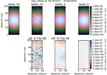
neg. offset at 791.875cm−1 (F18/cal04)

Figure 2.Real part of the NCO for different calibration methods at 791.875 cm−1. The leftmost image shows the BB-DS reference without pseudo-hyperbola fit. The following two are the values for the original BB-BB calibration and the corresponding hyperbola, and the last panel shows an application of the pseudo-hyperbola to the BB-DS calibration. The images in the second row show the difference between the NCO values and those for the BB-DS reference. An offset value given above a plot indicates that all values are to be understood as with this value subtracted.

trace gas retrieval algorithms. Because the IG and NCO func-tions are interdependent, updating the BB-BB IG with the corrected NCO removes similar structures from it, as shown in Fig. 3.

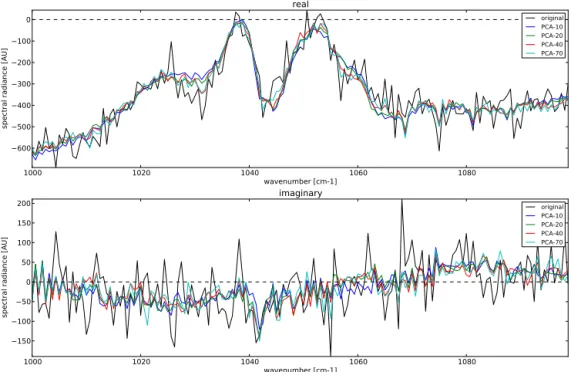
The pseudo-hyperbola function cannot reproduce the NCO for all spectral samples, as shown in Fig. 4 for the one at 840 cm−1. Here, the difference between the BB-DS NCO with and without the correction shows ring-like structures, which are likely related to emissions of the outer interferom-eter germanium window that peak around this wave number. However, the improvements to the BB-BB calibration over

the rest of the spectrum outweigh the cost of these artefacts, which only persist for a limited number of samples. Ongoing characterisation of the window emissions may eventually al-low the inclusion of window emissions as dedicated terms in the fit formula.

Following the L1 processing step, the spectra are currently averaged over one row to reduce stochastically independent noise for the L2 processing. For this application, the aver-age over each row of the NCO is an interesting diagnostic for the pseudo-hyperbola method. Figure 5 shows this quan-tity. Comparing the magnitude of the removed structures (of the order of 10−7W cm2_{cm sr}−1_{in the centre of the} detec-tor) with the magnitude of recorded atmospheric spectra, the artefacts would introduce a spatially uncorrelated error of up to nearly 8 % at this wave number for the BB-BB calibration unless corrected by the pseudo-hyperbola.

The size of this correction is attributable to two reasons. As mentioned above, the BB-BB calibration currently suf-fers from error magnification due to unexpectedly large and similar BB temperatures. A more fundamental reason is that the NCO itself is relatively large because the GLORIA spec-trometer operates at 200–220 K (Friedl-Vallon et al., 2014), and the radiative background can be comparable in magni-tude to atmospheric emissions, depending on the observed scene.

4 Calibration noise mitigation based on principal component analysis

4.1 Background and motivation

(6)

0 32 64 96 128 detector row bbds_nh bbbb_nh

0 24 48 detector column0

32 64 96 128 detector row off. -2.183 bbbb_h

0 24 48 detector column off. -2.183 bbds_h 2.50e-10 2.60e-10 2.70e-10 2.80e-10 2.90e-10 3.00e-10 3.10e-10 3.20e-10 3.30e-10 3.40e-10 3.50e-10 ma gn itu de (W cm − 2sr −

1cm AU

−

1)

0 24 48 detector column-5.00e+00

-4.00e+00 -3.00e+00 -2.00e+00 -1.00e+00 0.00e+00 1.00e+00 2.00e+00 3.00e+00 4.00e+00 5.00e+00

rel. diff. in mag. to bbds_nh (%)

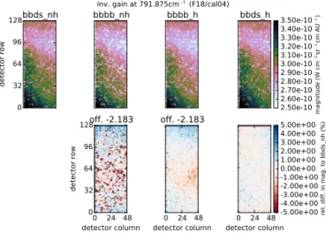
inv. gain at 791.875cm−1 (F18/cal04)

Figure 3.Magnitude of the IG for different calibration methods at 791.875 cm−1. The panels are laid out the same way as in Fig. 2. The variation from the lower left to the upper right corner is caused by a composition change in the detector material. An offset value given above a plot indicates that all values are to be understood as with this value subtracted.

0 32 64 96 128 detector row bbds_nh bbbb_nh

0 24 48 detector column 0 32 64 96 128 detector row off. 8.56e-08 bbbb_h

0 24 48 detector column off. 8.56e-08 bbds_h -2.00e-07 -6.00e-08 8.00e-08 2.20e-07 3.60e-07 5.00e-07 6.40e-07 7.80e-07 9.20e-07 1.06e-06 1.20e-06 rea l p art (W cm − 2sr − 1cm )

0 24 48 detector column -2.50e-07 -2.00e-07 -1.50e-07 -1.00e-07 -5.00e-08 0.00e+00 5.00e-08 1.00e-07 1.50e-07 2.00e-07 2.50e-07 diff. to bb ds_n h ( W cm − 2sr − 1cm )

Figure 4. Real part of the NCO at 840.00 cm−1, shown for the same calibration methods as in Fig. 2. Compared with the values at 791.875 cm−1, this spectral sample cannot be as accurately repro-duced using the pseudo-hyperbola fit. An offset value given above a plot indicates that all values are to be understood as with this value subtracted.

in these measurements stems from the instrument radiative background.

Let us assume that all pixels had the same response func-tion. We could then pretend that the individual spectra within a calibration image were a series of measurements from the same detector, each time exposed to a slightly varying scene. To put this in more mathematical terms, we have reason to suspect that the observed calibration scenes do not actually contain as many meaningful degrees of freedom as there are samples recorded by the instrument. If each of thenpixels’

0.0 3.5 7.0 10.5 14.0 real part (W cm−2sr−1cm)1e 7 0 32 64 96 128 detector row

bbbb_h

bbbb_nh

bbds_h

bbds_nh

5 0 5 10 15 20 25 diff. to bbds_nh (W cm−2sr−1cm)1e 8 0

32 64 96 128

Figure 5.Averaged real part of the NCO over the detector rows for the different calibration methods. Both the unmodified data (suffix nh) and the pseudo-hyperbolas (suffix h) are shown. A discrepancy remains between the BB-DS and BB-BB methods which has to be compensated for in the trace gas retrievals.

spectra consists of k partially correlated complex samples, this means we could find a way to instead represent it using a smaller but uncorrelated set ofK < k complex numbers. Such a transformation can be achieved by PCA (e.g. Joliffe, 2002). The PCA is a linear basis transformation yielding the original data in terms of a new orthonormal basis, composed of thek eigenvectors of its covariance matrix and sorted in order of decreasing contribution to the total variance. These vectors are the “principal components”. If the original data are noise normalised, such that the random noise becomes uncorrelated and uniform (white), any direction will carry the same amount of noise, so that reconstructing the data from a truncated set ofKcomponents will ideally reduce the sam-ple noise SDσ (ν)by a factor of

σk(ν)

σK(ν) =

r k

K. (8)

However, in practice, the relation holds true only asymptot-ically for largenbecause the ability to separate noise from signal depends on the number of measurements available for the decomposition (e.g. Pyatykh et al., 2013). A more realis-tic estimate, on the basis of a simulated white noise data set, will be shown in Sect. 4.3.

(7)

use of single- or averaged-image decomposition, as opposed to decomposition based on a training set of previous mea-surements. Note that PCA is usually formulated in a way that applies to real-valued data sets. In the following, we will use a straightforward generalisation to complex vector spaces. This has the implication that the covariance matrix of the data set is complex-valued, which makes it less read-ily interpreted. However, because the covariance matrix is self-adjoint, its main diagonal and its eigenvalues remain real numbers, so the components can still be ordered in the regu-lar fashion.

4.2 Data preconditioning and application of PCA

We start with a matrix X∈Cn×k _{containing either a BB}

or DS data set in Fourier transformed but not radiometri-cally calibrated form. The calibration data sets are obtained from averaging over all available single measurements of the same calibration source during one calibration sequence. The DS measurements have additionally been subjected to the trace gas emission removal technique (Kleinert et al., 2014). Again, nis the number of pixels, whilekis the number of spectral samples considered. In this section, we have chosen the spectral range between 780 and 1450 cm−1. The calibra-tion measurements are processed at the dynamics mode sam-pling of 0.625 cm−1; thereforek=_{1072. For technical}

rea-sons, the topmost line of pixels is not considered; therefore n=_6096.

The relation with the true radiance imageXˆ as seen by the detector can be expressed as

X=G⊙ ˆX, (9)

whereG∈Cn×k _{is the instrument gain matrix, and the} sym-bol⊙_{was chosen to represent the Hadamard (entrywise)}

ma-trix product. In the case whereXis a DS data set,Xˆ is domi-nated by the NCO, potentially with minor contributions from insufficiently removed residual trace gas signatures. IfXis a BB data set, the true image Xˆ contains the NCO and the nearly homogeneous blackbody radiation.

When PCA was introduced in Sect. 4.1, it was assumed that all pixels had the same response function, so that each pixel measured the same statistical variables. More practi-cally speaking, the set of pixel spectra resembled a series of measurements taken by the same instrument. This statisti-cal interpretation provides the notion of a covariance matrix, whose eigendecomposition PCA is based on. In order to be able to apply PCA for noise suppression, the data setX there-fore needs to be brought into a form which closely resembles this. To this end, the pixel response has to be homogenised; that is, the Hadamard inverse of the matrixGneeds to be ap-plied to the measurements. This poses a fundamental prlem, as the purpose of the calibration measurements is to ob-tain this matrix, and it is therefore naturally not known at this point.

We solve this problem by the following process. First, a smoothing of the blackbody and deep space measurements is performed based on singular value decomposition (SVD) without gain homogenisation, using 20 singular vectors for reconstruction. These spectra,X′_BBandX′_DSare now used to infer an approximation of the gain matrix:

G′=₈ eB⊙ X′_BB−X′_DS, (10) whereeBcontains the theoretically calculated inverse Planck radiances corresponding to the blackbody temperature. To avoid confusion with the ordinary matrix inverse, a tilde de-notes inversion with respect to the Hadamard product. For the purposes of homogenisation, multiplication with the inverse Planck radiances is not strictly necessary, but facilitates the physical interpretation of intermediate results. The function 8is a Kaiser window which acts as a smoothing function on each row of the matrix. Its purpose is to keep noise and signal variance out of the homogenisation matrix.

Using the entrywise inverse of the matrixG′, the black-body and deep space measurements can now be homogenised by gain calibration:

X′′=eG′⊙X′. (11)

To further reduce the variation that needs to be decom-posed by the PCA, the NCO pseudo-hyperbola from Sect. 3 is fitted to the gain calibrated deep space measurement at each spectral sample and then subtracted. Afterwards, the re-maining mean value of each spectral sample is computed and subtracted as well, yielding the new matrixX′′′.

This matrix now fulfills almost all the conditions neces-sary for the PCA. What is still missing is the normalisation of the individual spectral samples. Several methods exist to achieve this, the most simple of which being to divide each spectral sample by its sample SD. We opted for a method that approximates the spectral noise profile. A new recon-struction of the blackbody matrix is performed, based on the original decomposition, this time using 400 principal compo-nents. The difference between the original spectrum and the reconstructed spectrum is then used to normalise the noise variance of the matrixX′′′, under the assumption that the re-construction residual can be used as a proxy for the noise profile:

Y=X′′′N−1, (12)

whereN∈Rk×k_{contains the SD of the calculated difference} on the main diagonal. Note that this is not an approximation of the total noise, but only of the spectral distribution for the purpose of rescaling. To arrive at the full noise, a more thor-ough analysis is necessary (Antonelli et al., 2004). TheN matrix is computed separately for DS and BB measurements. Finally, the PCA is performed onYby way of a complex SVD:

(8)

800 900 1000 1100 1200 1300 1400 wavenumber [cm-1]

500 0 500 1000

spectral radiance [AU]

real

original PCA-10 PCA-20 PCA-40 PCA-70

800 900 1000 _{wavenumber [cm-1]}1100 1200 1300 1400

200 0 200 400 600

imaginary

Figure 6.Reconstruction of a DS spectrum (centre pixel) from 10, 20, 40, and 70 principal components.

Here, U∈Cn×n _and_V_∈_Ck×k _{contain the left- and}

right-singular vectors, respectively, and S∈Cn×k _{is a}

rectangu-lar diagonal matrix which contains the singurectangu-lar values. The squares of the singular values are eigenvalues of the covari-ance matrix Y∗Y, the rows of V∗ contain the orthonormal eigenvectors and the rows of the productT=UScontain the linear factors, i.e. the coordinates of each row ofYin the new basis defined byV. A truncated reconstructionXK ofX

us-ingK covariance eigenvectors can now be obtained by first reconstructingYusing truncated matricesSK andVK, then

inverting the normalisation steps performed before.

After the procedure is finished, it is repeated once, starting with the original data setX. The new decomposition (13) for the BB and DS measurements is now used instead of the ini-tial SVD to estimate the gain matrix and pseudo-hyperbola more accurately. An iterative approach using successive rep-etitions of the procedure was considered, but did not yield improved results.

4.3 Reconstruction from principal components

With the PCA calculated, the DS and BB spectra can be re-constructed using a chosen number of principal components. The more components are used, the more exactly the original data are reconstructed, the signal as well as the noise. Several diagnostics can be used to help decide on a sensible number of components to include.

The first diagnostic is visual inspection of the recon-structed spectra. As an example, a DS data set and a BB data set from the ESMVal campaign have been subjected to the PCA method. The original data sets were obtained by

aver-aging the available calibration measurements from a calibra-tion sequence recorded on 23 September 2012. The DS mea-surements were recorded at full resolution, and then the it-erative DS correction procedure was applied to remove trace gas emissions from the upper atmosphere. Afterwards, the measurements were reduced to DM resolution, i.e. a spectral sampling of 0.625 cm−1, the same as the blackbody measure-ments. Prior to the processing, both spectra were rotated so that their phase angle in the complex plane is approximately that of a calibrated spectrum. This is not necessary for the procedure, but helps with the physical interpretation of the real and imaginary parts.

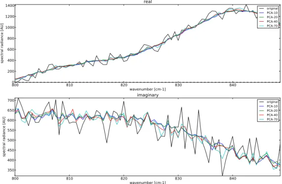
Figures 6 and 7 show the full reconstructions of the DS and BB, respectively, from 10, 20, 40, and 70 principal com-ponents. Both spectra are reproduced well on this scale. In order for the differences to become more apparent, both be-tween the different reconstructions and bebe-tween the recon-struction and the original, we will concentrate on the DS spectrum within limited spectral ranges.

(9)

800 900 1000 1100 1200 1300 1400 wavenumber [cm-1]

5000 10000 15000 20000 25000 30000 35000

real

800 900 1000 _{wavenumber [cm-1]}1100 1200 1300 1400

30 20 10 0 10 20 30

imaginary

Figure 7.Reconstruction of a BB spectrum (centre pixel) from 10, 20, 40, and 70 principal components.

800 810 820 830 840

wavenumber [cm-1] 0

200 400 600 800 1000 1200 1400

real

800 810 820 830 840

wavenumber [cm-1] 350

400 450 500 550 600 650 700

imaginary

Figure 8.The same reconstructions as in Fig. 6 but in a limited spectral range between 800 and 850 cm−1.

any case, the contaminated spectral range cannot be used, so the quality of its reconstruction is not crucial.

4.4 Covariance eigenvalues

Another avenue for diagnostics is provided by inspection of the singular valuessi, i.e. the main diagonal elements of the

matrix S from Eq. (13), whose squares are the covariance

(10)

1000 1020 1040 1060 1080 wavenumber [cm-1]

600 500 400 300 200 100 0

real

1000 1020 1040_{wavenumber [cm-1]} 1060 1080

150 100 50 0 50 100 150 200

imaginary

Figure 9.Reconstructions of the same DS spectrum as in Figs. 6 and 8, in the spectral range between 1000 and 1100 cm−1. The obvious discrepancies between the reconstructions and the original spectrum are due to residual emissions from stratospheric trace gases.

variance of each variable restored in the reconstruction:

σ_K2 σ2 =

K

P

i=1

s_i2

k

P

i=1

s_i2

=tr(S

T KSK)

tr(ST_S₎ . (14)

As was mentioned in Sect. 4.1, the distribution of white noise among the PCA vectors depends on the dimensionality of the data set. To estimate the performance of our method, we have generated a matrixXsyn∈C6096×1072. The real and imaginary parts of the matrix entries were drawn indepen-dently from a standard normal distribution.

Figure 10 shows the first 70 normalised covariance eigen-values for the DS spectrum from Fig. 6, the BB data set from Fig. 7, and the white noise matrixXsyn. The cumulative sum of the first 30 eigenvalues is shown in Fig. 11.

For the DS spectra, the first five principal components al-ready account for more than half of the variation in the mea-surement. Using 20 vectors, this figure increases to 60 %. It should be noted here that this is the variance after the ho-mogenisation procedure; that is, most of the variation over the detector has already been removed. The spectrum recon-structed here is a combination of the detector noise, a correc-tion to the assumed pseudo-hyperbola shape in the real part and the imaginary part of the spectrum.

The BB data set can be reconstructed to 90 % of the total variance from as few as 14 principal components. Because the BB spectra contain the same background as the DS as well as the much brighter blackbody radiation, the total

vari-ance is higher. However, the blackbody radiation, which ac-counts for most of the signal, is easily reconstructed due to its homogeneity.

The synthetic noise is reconstructed much more linearly than the BB and DS measurements, but the covariance eigen-values still decrease slightly for successive components. This is the expected non-uniform noise distribution which moti-vated the simulation. The contribution of successive princi-pal components starts at 0.19 % and decreases to 0.16 % for the 70th component. The last eigenvalue (not shown in the plots) is 3.2×10−4, an order of magnitude smaller than the first one. The mean eigenvalue is 1/1072≈₉.3×₁₀−4_{, the} expected contribution of each single component if the noise variance was distributed evenly.

4.5 Comparison with low-pass filtering

Another useful method for noise mitigation of GLORIA cal-ibration measurements is a simple low-pass filtering (LPF) of the spectra. Note that, in this context, LPF refers to low and high frequencies in the Fourier space associated with the spectrum, not with the recorded signal. This space can be identified with the interferogram space. Applying an LPF to the spectrum is therefore equivalent to a shortening of the interferogram in combination with a Fourier interpolation of the spectrum.

(11)

Figure 10.Normalised covariance eigenvalues of a DS, BB, and synthetic white noise data set. The eigenvalues indicate the rate at which each successive principal component adds to the total vari-ance.

is achieved is different. The BB and DS measurements con-tain the instrument background and calibration blackbody ra-diation, both of which are spectrally slowly varying signals without discernible emission or absorption lines. This mo-tivates and justifies the use of the LPF, which discards the higher frequencies, i.e. the rapidly varying components, be-cause they can be expected to contain little or no signal but contribute equally to the noise level. The PCA method de-composes the data into uncorrelated components and retains only the most significant ones, discarding those that con-tribute little to the total variance of each spectral sample.

Because of the qualitatively different effects the two meth-ods have on the data, a quantitative comparison of PCA and LPF proved difficult. In the following, we will make a qual-itative comparison between a PCA reconstruction from 20 principal components (PCA-20) and a low-pass filter which dampens all but the 512 lowermost frequencies (LPF-512). As Fig. 11 shows, the first 20 PCA vectors reconstruct the simulated noise variance to 3.6 %, implying a reduction of the noise SD by over 80 %.

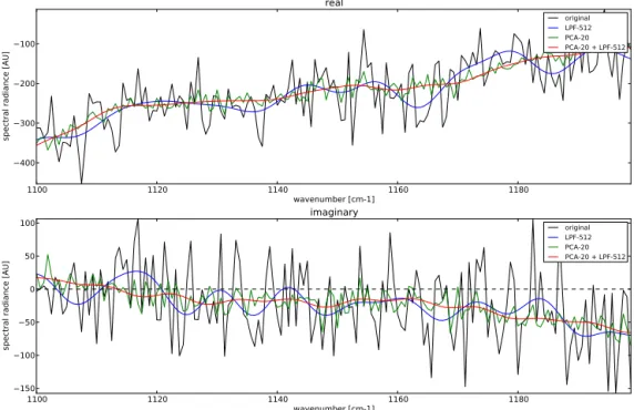
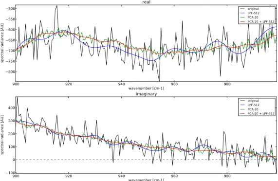
Figure 12 shows a reconstruction of a spectrum subjected to the PCA-20 and LPF-512 methods, as well as a third one, where the signal was first reconstructed from the principal components and subsequently low-pass-filtered. For a more detailed inspection of the differences, Figs. 14 and 13 show the same spectra within a reduced wave-number range.

The LPF-512 method effectively reduces the interfero-gram length from 8000 to 1024 real samples; that is, it retains 512 of 4001 complex modes. Assuming a uniform noise dis-tribution among the modes, this implies a noise level reduc-tion of 2.8:_{1, while for the PCA-20 method we expect a ratio}

of 5:_{1 from the simulation in Sect. 4.4. A more}

fundamen-tal difference, regardless of the number of principal

compo-Figure 11.Cumulative normalised covariance eigenvalues, i.e. the cumulative sum of the values shown in Fig. 10. These indicate the relative variance restored after reconstructing the image from a given number of principal components.

nents, is that the noise removed by the PCA method does not have a high-frequency bias, which is why the smoothing effect is less pronounced.

This difference between the PCA and low-pass methods is further illustrated by Fig. 15, which shows the magnitude of the complex reconstruction residual in Fourier space, for the LPF-512, PCA-20 and combined methods. The reconstruc-tion residual for the pure low-pass method is an order of mag-nitude smaller for the lowermost frequencies, corresponding to the low-pass window employed. The PCA method, on the other hand, distributes the reconstruction residual more uni-formly across the spectrum. This is also true for the com-bined method as long as the number of principal components is small. For larger numbers, the PCA-reconstructed spec-trum approaches the original specspec-trum and the combined re-construction according to the LPF-512 method.

The benefit of the combined approach is that most of the noise variance is already subtracted before the low pass is applied, and therefore the undesired interpolation of the low-frequency noise modes is avoided. This results in a smooth calibration spectrum without the smoothing artefacts in the shape of slow oscillations.

5 Conclusions and outlook

One of the GLORIA limb sounder’s key features is its imag-ing capability. In this paper, we presented two new ways to exploit this feature for the suppression of noise and certain artefacts in the calibration measurements.

(12)

calibra-800 900 1000 1100 1200 1300 1400 wavenumber [cm-1]

500 0 500 1000

real

original LPF-512 PCA-20 PCA-20 + LPF-512

800 900 1000 _{wavenumber [cm-1]}1100 1200 1300 1400

200 0 200 400 600

imaginary

Figure 12.Comparison between the PCA, low-pass and combined noise suppression methods, applied to the same DS measurement as in Fig. 6.

1100 1120 1140_{wavenumber [cm-1]} 1160 1180

400 300 200 100

real

1100 1120 1140 1160 1180

wavenumber [cm-1] 150

100 50 0 50 100

imaginary

Figure 13.Comparison between the PCA, low-pass and combined noise suppression methods (cf. Fig. 12) in the spectral range between 1100 and 1200 cm−1. The pure low-pass method retains higher amounts of low-frequency noise, which manifest as slow oscillations in the spectrum. The PCA method subtracts noise variance irrespective of frequency (see also Fig. 15).

tion measurements and an imperfect nonlinearity correction. Fitting a pseudo-hyperbola to the gain-calibrated radiometric offset allows us to use both blackbodies to generate calibra-tion data of decent quality. Without the fit, the amplificacalibra-tion

(13)

900 920 940 960 980 wavenumber [cm-1]

800 750 700 650 600 550 500

real

900 920 940 _{wavenumber [cm-1]} 960 980

100 0 100 200 300 400

imaginary

Figure 14.Comparison between the PCA, low-pass and combined noise suppression methods (cf. Fig. 12) in a limited spectral range. Between 920 and 960 cm−1, a visible difference appears between the PCA methods and the pure LPF method. This difference is still within the original spectrum’s noise range.

0.00 0.05 0.10 0.15 0.20 0.25 0.30

frequency [cm] 101

102 103 104

reconstruction residual magnitude [AU]

LPF-512 PCA-20 PCA-20 + LPF-512 PCA-600 + LPF-512

Figure 15.Spectrum of the reconstruction residual, i.e. the differ-ence between the processed and original spectra, for different noise suppression methods. Shown are only the low frequencies. The LPF subtracts high-frequency noise from the spectrum, which means that low-frequency noise modes are retained. The PCA method intro-duces no such bias. The combined PCA+LPF method introduces no noticeable bias as long as the number of principal components is kept small. Note that the abscissa is in spatial units; this is because it is the Fourier space associated with the wave-number space.

We could significantly reduce the noise level of BB and DS calibration spectra by exploiting the spectral correlation of GLORIA’s calibration scenes. Via truncated PCA, we were able to reconstruct the original measurements while reduc-ing the noise level significantly. Compared with low-pass smoothing, an alternative option for GLORIA spectra, the PCA reconstruction is less smooth, but subtracts high- and low-frequency noise variance equally. By contrast, low-pass filters retain the low-frequency noise components, resulting in slowly oscillating perturbations in the result. A combined approach, where a low-pass smoothing is performed on pre-viously PCA-compressed spectra, yielded the best results with suppressed low-frequency noise.

We expect that the techniques presented in this paper can also be adapted to other instruments with a focal plane ar-ray and similar absolute radiance calibration. The utility of the PCA-based method for other instruments would likely depend on the number of pixels available for each measure-ment, as well as the homogeneity of the calibration scenes.

(14)

Acknowledgements. The GLORIA instrument was mainly funded by the Helmholtz Association. We thank the whole GLORIA instrument team for their role in developing the hardware and software, as well as planning and executing the measurement campaigns. Acknowledgments also go to Myasishchev Design Bureau and the German Aerospace Centre (DLR-FX), who operate GLORIA’s carrier aircraft.

The article processing charges for this open-access publication were covered by a Research

Centre of the Helmholtz Association.

Edited by: J. Notholt

References

Antonelli, P., Revercomb, H. E., Sromovsky, L. A., Smith, W. L., Knuteson, R. O., Tobin, D. C., Garcia, R. K., Howell, H. B., Huang, H.-L., and Best, F. A.: A principal component noise filter for high spectral resolution infrared measurements, J. Geophys. Res., 109, D23102, doi:10.1029/2004JD004862, 2004.

August, T., Klaes, D., Schlüssel, P., Hultberg, T., Crapeau, M., Ar-riaga, A., O’Carroll, A., Coppens, D., Munro, R., and Calbet, X.: IASI on Metop-A: operational Level 2 retrievals after five years in orbit, J. Quant. Spectrosc. Ra., 113, 1340–1371, 2012. Beer, R.: Remote Sensing by Fourier Transform Spectrometry, vol.

170, Wiley-Interscience, New York, 1–14, 1992.

Fischer, H., Birk, M., Blom, C., Carli, B., Carlotti, M., von Clar-mann, T., Delbouille, L., Dudhia, A., Ehhalt, D., EndeClar-mann, M., Flaud, J. M., Gessner, R., Kleinert, A., Koopman, R., Langen, J., López-Puertas, M., Mosner, P., Nett, H., Oelhaf, H., Perron, G., Remedios, J., Ridolfi, M., Stiller, G., and Zander, R.: MIPAS: an instrument for atmospheric and climate research, Atmos. Chem. Phys., 8, 2151–2188, doi:10.5194/acp-8-2151-2008, 2008. Friedl-Vallon, F., Maucher, G., Seefeldner, M., Trieschmann, O.,

Kleinert, A., Lengel, A., Keim, C., Oelhaf, H., and Fischer, H.: Design and characterization of the balloon-borne Michelson In-terferometer for Passive Atmospheric Sounding (MIPAS-B2), Appl. Optics, 43, 3335–3355, 2004.

Friedl-Vallon, F., Gulde, T., Hase, F., Kleinert, A., Kulessa, T., Maucher, G., Neubert, T., Olschewski, F., Piesch, C., Preusse, P., Rongen, H., Sartorius, C., Schneider, H., Schönfeld, A., Tan, V., Bayer, N., Blank, J., Dapp, R., Ebersoldt, A., Fischer, H., Graf, F., Guggenmoser, T., Höpfner, M., Kaufmann, M., Kretschmer, E., Latzko, T., Nordmeyer, H., Oelhaf, H., Orphal, J., Riese, M., Schardt, G., Schillings, J., Sha, M. K., Suminska-Ebersoldt, O., and Ungermann, J.: Instrument concept of the imaging Fourier transform spectrometer GLORIA, Atmos. Meas. Tech., 7, 3565– 3577, doi:10.5194/amt-7-3565-2014, 2014.

Frigo, M. and Johnson, S. G.: FFTW: an adaptive software architec-ture for the FFT, in: Proceedings of the 1998 IEEE International Conference on Acoustics, Speech and Signal Processing, vol. 3, 1381–1384, IEEE, 1998.

Gettelman, A., Hoor, P., Pan, L., Randel, W., Hegglin, M., and Birner, T.: The extratropical upper troposphere and lower stratosphere, Rev. Geophys., 49, RG3003, doi:10.1029/2011RG000355, 2011.

Grossmann, K. U., Offermann, D., Gusev, O., Oberheide, J., Riese, M., and Spang, R.: The CRISTA-2 mission, J. Geophys. Res., 107, CRI 1–1–CRI 1–12, doi:10.1029/2001JD000667, 2002.

Guggenmoser, T.: Data Processing and Trace Gas Retrievals for the GLORIA Limb Sounder, vol. 230 of Schriften des Forschungszentrums Jülich, Reihe Energie und Umwelt, Forschungszentrum Jülich GmbH, Jülich, 70–76, 2014. Hoffmann, L., Kaufmann, M., Spang, R., Müller, R., Remedios,

J. J., Moore, D. P., Volk, C. M., von Clarmann, T., and Riese, M.: Envisat MIPAS measurements of CFC-11: retrieval, vali-dation, and climatology, Atmos. Chem. Phys., 8, 3671–3688, doi:10.5194/acp-8-3671-2008, 2008.

Höpfner, M., Stiller, G. P., Kuntz, M., von Clarmann, T., Echle, G., Funke, B., Glatthor, N., Hase, F., Kemnitzer, H., and Zorn, S.: The Karlsruhe optimized and precise radiative transfer algorithm. Part II: Interface to retrieval applications, in: Optical Remote Sensing of the Atmosphere and Clouds, Beijing, China, 15–17 September 1998, edited by: Wang, J., Wu, B., Ogawa, T., and Guan, Z., vol. 3501, 186–195, 1998.

Joliffe, I. T.: Principal Component Analysis, Springer Series in Statistics, Springer, Berlin, 2nd edn., 2002.

Kalicinsky, C., Grooß, J.-U., Günther, G., Ungermann, J., Blank, J., Höfer, S., Hoffmann, L., Knieling, P., Olschewski, F., Spang, R., Stroh, F., and Riese, M.: Observations of filamentary struc-tures near the vortex edge in the Arctic winter lower stratosphere, Atmos. Chem. Phys., 13, 10859–10871, doi:10.5194/acp-13-10859-2013, 2013.

Kaufmann, M., Blank, J., Guggenmoser, T., Ungermann, J., En-gel, A., Ern, M., Friedl-Vallon, F., Gerber, D., Grooß, J. U., Guenther, G., Höpfner, M., Kleinert, A., Kretschmer, E., Latzko, Th., Maucher, G., Neubert, T., Nordmeyer, H., Oelhaf, H., Olschewski, F., Orphal, J., Preusse, P., Schlager, H., Schneider, H., Schuettemeyer, D., Stroh, F., Suminska-Ebersoldt, O., Vogel, B., M. Volk, C., Woiwode, W., and Riese, M.: Retrieval of three-dimensional small-scale structures in upper-tropospheric/lower-stratospheric composition as measured by GLORIA, Atmos. Meas. Tech., 8, 81–95, doi:10.5194/amt-8-81-2015, 2015. Kleinert, A. and Trieschmann, O.: Phase determination for a Fourier

transform infrared spectrometer in emission mode, Appl. Optics, 46, 2307–2319, doi:10.1364/AO.46.002307, 2007.

Kleinert, A., Friedl-Vallon, F., Guggenmoser, T., Höpfner, M., Neu-bert, T., Ribalda, R., Sha, M. K., Ungermann, J., Blank, J., Eber-soldt, A., Kretschmer, E., Latzko, T., Oelhaf, H., Olschewski, F., and Preusse, P.: Level 0 to 1 processing of the imaging Fourier transform spectrometer GLORIA: generation of radiometrically and spectrally calibrated spectra, Atmos. Meas. Tech., 7, 4167– 4184, doi:10.5194/amt-7-4167-2014, 2014.

Kullmann, A., Riese, M., Olschewski, F., Stroh, F., and Gross-mann, K. U.: Cryogenic infrared spectrometers and telescopes for the atmosphere – new frontiers, in: Proc. SPIE, vol. 5570, 423–432, doi:10.1117/12.564856, 2004.

Monte, C., Gutschwager, B., Adibekyan, A., Kehrt, M., Ebersoldt, A., Olschewski, F., and Hollandt, J.: Radiometric calibration of the in-flight blackbody calibration system of the GLORIA inter-ferometer, Atmos. Meas. Tech., 7, 13–27, doi:10.5194/amt-7-13-2014, 2014.

(15)

Telescopes for the Atmosphere (CRISTA) experiment and mid-dle atmosphere variability, J. Geophys. Res., 104, 16311–16325, 1999.

Olschewski, F., Ebersoldt, A., Friedl-Vallon, F., Gutschwager, B., Hollandt, J., Kleinert, A., Monte, C., Piesch, C., Preusse, P., Rolf, C., Steffens, P., and Koppmann, R.: The in-flight blackbody calibration system for the GLORIA interferometer on board an airborne research platform, Atmos. Meas. Tech., 6, 3067–3082, doi:10.5194/amt-6-3067-2013, 2013.

Piesch, C., Gulde, T., Sartorius, C., Friedl-Vallon, F., Seefeld-ner, M., Wölfel, M., Blom, C., and Fischer, H.: Design of a MIPAS instrument for high-altitude aircraft, in: Presented at the Second International Airborne Remote Sensing Conference and Exhibition, vol. 24, p. 27, 1996.

Pyatykh, S., Hesser, J., and Zheng, L.: Image noise level estimation by principal component analysis, IEEE T. Image Process., 22, 687–699, doi:10.1109/TIP.2012.2221728, 2013.

Revercomb, H. E., Buijs, H., Howell, H. B., LaPorte, D. D., Smith, W. L., and Sromovsky, L.: Radiometric calibration of IR Fourier transform spectrometers: solution to a problem with the High-Resolution Interferometer Sounder, Appl. Optics, 27, 3210–3218, 1988.

Riese, M., Preusse, P., Spang, R., Ern, M., Jarisch, M., Gross-mann, U., and OfferGross-mann, D.: Measurements of trace gases by the Cryogenic Infrared Spectrometers and Telescopes for the At-mosphere (CRISTA) experiment, Adv. Space Res., 19, 563–566, doi:10.1016/S0273-1177(97)00172-5, 1997.

Riese, M., Manney, G. L., Oberheide, J., Tie, X., Spang, R., and Küll, V.: Stratospheric transport by planetary wave mix-ing as observed durmix-ing CRISTA-2, J. Geophys. Res., 107, 8179, doi:10.1029/2001JD000629, 2002.

Riese, M., Oelhaf, H., Preusse, P., Blank, J., Ern, M., Friedl-Vallon, F., Fischer, H., Guggenmoser, T., Höpfner, M., Hoor, P., Kauf-mann, M., Orphal, J., Plöger, F., Spang, R., Suminska-Ebersoldt, O., Ungermann, J., Vogel, B., and Woiwode, W.: Gimballed Limb Observer for Radiance Imaging of the Atmosphere (GLO-RIA) scientific objectives, Atmos. Meas. Tech., 7, 1915–1928, doi:10.5194/amt-7-1915-2014, 2014.

Solomon, S., Rosenlof, K. H., Portmann, R. W., Daniel, J. S., Davis, S. M., Sanford, T. J., and Plattner, G.-K.: Con-tributions of stratospheric water vapor to decadal changes in the rate of global warming, Science, 327, 1219–1223, doi:10.1126/science.1182488, 2010.

Stiller, G. P. (Ed.): The Karlsruhe Optimized and Precise Radiative Transfer Algorithm (KOPRA), vol. 6487 of Wissenschaftliche Berichte des Forschungszentrums Karlsruhe, Forschungszen-trum Karlsruhe, Karlsruhe, 2000.

Ungermann, J., Kaufmann, M., Hoffmann, L., Preusse, P., Oelhaf, H., Friedl-Vallon, F., and Riese, M.: Towards a 3-D tomographic retrieval for the air-borne limb-imager GLORIA, Atmos. Meas. Tech., 3, 1647–1665, doi:10.5194/amt-3-1647-2010, 2010. Ungermann, J., Blank, J., Lotz, J., Leppkes, K., Hoffmann, L.,

Guggenmoser, T., Kaufmann, M., Preusse, P., Naumann, U., and Riese, M.: A 3-D tomographic retrieval approach with advec-tion compensaadvec-tion for the air-borne limb-imager GLORIA, At-mos. Meas. Tech., 4, 2509–2529, doi:10.5194/amt-4-2509-2011, 2011.

Ungermann, J., Kalicinsky, C., Olschewski, F., Knieling, P., Hoff-mann, L., Blank, J., Woiwode, W., Oelhaf, H., Hösen, E., Volk, C. M., Ulanovsky, A., Ravegnani, F., Weigel, K., Stroh, F., and Riese, M.: CRISTA-NF measurements with unprecedented ver-tical resolution during the RECONCILE aircraft campaign, At-mos. Meas. Tech., 5, 1173–1191, doi:10.5194/amt-5-1173-2012, 2012.

Ungermann, J., Pan, L. L., Kalicinsky, C., Olschewski, F., Kniel-ing, P., Blank, J., Weigel, K., Guggenmoser, T., Stroh, F., Hoff-mann, L., and Riese, M.: Filamentary structure in chemical tracer distributions near the subtropical jet following a wave breaking event, Atmos. Chem. Phys., 13, 10517–10534, doi:10.5194/acp-13-10517-2013, 2013.

Ungermann, J., Blank, J., Dick, M., Ebersoldt, A., Friedl-Vallon, F., Giez, A., Guggenmoser, T., Höpfner, M., Jurkat, T., Kauf-mann, M., KaufKauf-mann, S., Kleinert, A., Krämer, M., Latzko, T., Oelhaf, H., Olchewski, F., Preusse, P., Rolf, C., Schillings, J., Suminska-Ebersoldt, O., Tan, V., Thomas, N., Voigt, C., Zahn, A., Zöger, M., and Riese, M.: Level 2 processing for the imag-ing Fourier transform spectrometer GLORIA: derivation and val-idation of temperature and trace gas volume mixing ratios from calibrated dynamics mode spectra, Atmos. Meas. Tech., 8, 2473– 2489, doi:10.5194/amt-8-2473-2015, 2015.

Weigel, K., Hoffmann, L., Günther, G., Khosrawi, F., Olschewski, F., Preusse, P., Spang, R., Stroh, F., and Riese, M.: A strato-spheric intrusion at the subtropical jet over the Mediterranean Sea: air-borne remote sensing observations and model results, Atmos. Chem. Phys., 12, 8423–8438, doi:10.5194/acp-12-8423-2012, 2012.