Effects of disorder on the dynamics of the XY chain

(1)

Effects of disorder on the dynamics of the

_XY

chain

Maria Eugenia Silva Nunes*

Departamento de Fı´sica, Universidade Federal de Minas Gerais, 30.123-970 Belo Horizonte, Minas Gerais, Brazil

Joa˜o Florencio†

Instituto de Fı´sica, Universidade Federal Fluminense, 24.210-340 Nitero´i, Rio de Janeiro, Brazil ~Received 7 February 2003; revised manuscript received 2 May 2003; published 7 July 2003!

We investigate the effects of disorder on the dynamics of thes51/2XYmodel in one dimension. The energy couplings are randomly drawn independently from a bimodal distribution. We use an extension of the method of recurrence relations, in which an averaging over realizations of disorder is incorporated into the definition of the scalar product of the dynamical Hilbert space ofsj

z₍

t), to determine analytically the first six basis vectors as well as the corresponding recurrants. We then use an ansatz for the higher-order recurrants, based on the behavior of the first ones exactly determined, to obtain the time-dependent correlation functions and spectral densities for several degrees of disorder. We find that the dynamics at long times is governed by the stronger couplings present in the system even if only a very small amount of disorder is present. In the long-time limit, the correlation functions oscillate at the cutoff frequency of the disorderless stronger-coupling case, with the spectral densities displaying tails that end at the stronger-coupling cutoff frequency.

DOI: 10.1103/PhysRevB.68.014406 PACS number~s!: 75.40.Gb, 75.50.Lk, 75.10.Jm, 75.10.Pq

I. INTRODUCTION

The behavior of disordered quantum spin chains has been of considerable theoretical interest in the the past two decades.1–3Most of the work, though, deals with phase dia-grams, ground-state properties, thermodynamic functions, etc. Not much attention has been paid to the study of Hamil-tonian dynamics in such systems. Only recently, calculations of dynamic correlation functions have been reported for some disordered quantum spin chains.4 – 6 In this work, we investigate the effects of disorder on the dynamics of theXY model7,8 in the high-temperature limit. We are interested in both the time-dependent spin-correlation functions and the spectral functions in the presence of disorder.

There exist studies in the literature which deal with dy-namic correlation functions of disorderless spin chains. There are only a few exact solutions in the infinite tempera-ture limit. For the XY model, the time-dependent longitudi-nal spin autocorrelation function is known since the work of Niemeijer9 to behave as the squared Bessel function, J0(2Jt)2, where Jis the nearest-neighbor energy coupling. On the other hand, the transverse autocorrelation function has an exact solution as a Gaussian.10–13Some exact results were also reported for finite temperatures.14The dynamics of the surface x-component spin in a semi-infinite XY chain was exactly determined by Sen.15 There is also an exact so-lution by Stolzeet al.16for the spin-autocorrelation functions of the first few spins of the semi-infinite XY model in one dimension at infinite temperature. Although some works have appeared in the literature for theXY chain with a single impurity,17,18the dynamics of the model with arbitrary con-centration of disorder is still not understood.

The XY model is defined by the Hamiltonian

H521

2 i

(

51 N

Ji~si x

si11 x

1si y

si11 y

!, ~1!

where si

a

are Pauli matrices at sites i, a5x,y,z. Ji are

nearest-neighbor coupling constants andN is the number of spins. We assume periodic boundary conditions, that is,

si1N

a

5si

a

. In this work, we consider the coupling energies between neighboring sites as random variables that can take the valuesJAorJB. The couplings are drawn independently

from the bimodal distribution

r~$Ji%!5

)

i N

@~12p!d~Ji2JA!1pd~Ji2JB!#, ~2!

where 0<p<1, p representing the fraction of JB bonds.

Since Eq. ~2!is normalized to unity, the average over disor-der realizations of a given quantity f($Ji%) is given by

f~$Ji%!5

E

2` `

r~$Ji%!f~$Ji%!

)

i N

dJi. ~3!

Our main quantity of interest, the time-dependent correla-tion funccorrela-tion, is defined by

C~t!5^si z

~0!si z

~t!

&

, ~4!

where

^

•••

&

denotes an ensemble average followed by an average over the disorder variables. We use the method of recurrence relations19–26 to obtain the short-time expansion of C(t) and a continued-fraction analysis to extend the re-sults to the long-time region. The rere-sults are then used in the calculation of the spectral densities.

(2)

make the correlation function to behave like its analog in a given pure stronger-coupling chain at the long-time limit.

This paper is arranged as follows. In Sec. II, we review the method of recurrence relations employed here to include disorder, and in Sec. III the method is used to obtain the dynamic longitudinal correlation functions of the XY model for different amounts of disorder. Finally, in Sec. IV we sum-marize our results.

II. METHOD OF RECURRENCE RELATIONS

The time evolution of a Hermitian operatorAin a system described by a HamiltonianHis governed by the equation of motion

dA~t!

dt 5iLA~t!, ~5!

where L is the Liouville operator,LA5@H,A#[HA2AH. The solution to Eq. ~5!is cast in the form of the orthogonal expansion,

A~t!5

(

n50

d21

an~t!fn, ~6!

where fn are orthogonal basis vectors spanning a d-dimensional Hilbert spaceS.

In order to account for disorder, the scalar product is de-fined as the Kubo product averaged over the realizations of the disorder.5Accordingly, it reads

~X,Y!5_b1

E

0 b

dl

^

X~ l !Y†

&

2^X

&^

Y†

&

, ~7!

where X and Y are vectors defined in S, b51/kBT is the

inverse temperature, andX(l)5exp(lH)Xexp(2lH). In the high-temperature limit,T_→`, the scalar product becomes

~X,Y!5TrXY†/Z, ~8! where the partition function Z now yields the number of quantum states of the systemZ5Tr 1. In the case of spin-1/2 models, Z52N, where N is the number of spins in the system.

By choosing f₀5A(0), it follows from Eq. ~6! that a₀(0)51 anda_n(0)50 forn>1. Furthermore, the remain-ing basis vectors are generated by the recurrence relation ~RRI!

fn115iL fn1Dnfn21, 0<n<d21, ~9! where

Dn5

~fn,fn!

~fn21,fn21!

, n<1 ~10!

are the relative norms of basis vectors, also known as recurrants.19 By definition, f₂1[0 and D0[1. The coeffi-cients an(t), which are the relaxation functions, satisfy a

second recurrence relation ~RRII!

Dn11an11~t!52 dan~t!

dt 1an21~t!, 0<n<d21, ~11!

where a₂1(t)[0. Hence, a0(t) represents the relaxation function of linear-response theory. In the limitT_→`, a₀(t) is simply the time-dependent autocorrelation function

^

A(0)A(t)

&

.

Thus, the complete time evolution of A(t) can be deter-mined from RRI and RRII. By taking the Laplace transform of the recurrence relation RRII, one obtains

D1a1~z!512za0~z!, n50, ~12! D_n₁₁an11~z!52zan~z!1an21~z!, n>1, ~13! where

an~z!5

E

0

`

exp~2zt!a_n~t!dt Rez

&

0. ~14!

It follows from Eqs. ~12!and~13!thata0(z) can be cast in the continued-fraction form

a₀~z!5 1

z1

D₁

z1

D₂ z1•••

. ~15!

Note that the recurrants Dn are the sole ingredients that

enter the determination of the dynamic correlation functions. In addition, the knowledge of Dn enables one to obtain the

moments of the spectral density,

m2k5

1 Z Trsi

z

@H,†H, . . .@H,si z

#. . .‡#, ~16! in which there are 2k nested commutators. The moments can be used to obtain the Taylor time series expansion for the correlation function in the infinite temperature limit as follows:

C~t!5

(

k50

`

~21!k

~2k!! m2kt

2k_. _~17!

Usually, only a fewDncan be determined analytically, since

the calculation of higher-order recurrants can be too lengthy or time consuming. Even though the moments enter in a simple manner in the correlation functions, it is preferable to inspect the behavior of the recurrants in order to devise any extrapolation scheme.

There are several types of approximations found in the literature to estimate the time-dependent correlation func-tions based on the limited information contained in just a few moments ~or recurrants!. One can truncate the continued fraction fora0(z) by introducing a terminating function. Ex-amples are the n-pole approximations27 and the Gaussian terminator.28

(3)

recur-rants, and the truncation uses as many recurrants as is com-putationally feasible. In this way, one can manage to obtain results which are valid at longer times. In any event, once the ansatz of recurrants is chosen, one is able to obtain readily the corresponding moments, since there are as many non-trivial moments as there are recurrants. In this way, one ob-tains the first coefficients of the short-time expansion for C(t) from the knowledge of the moments. In general, one could extend the region of validity in time by constructing Pade´ approximants to the full time series or by using other extrapolation schemes.30We do not find it necessary to em-ploy any of those methods, since we already use as many short-time coefficients from the ansatz as we can to obtain sensible results numerically. In the present work, we shall adopt the following strategy. First, after examining the struc-ture of the recurrants, we will put forward a model for the remaining Dn. From these we will get the first short-time

coefficients of C(t). Finally, the spectral densityF(v), de-fined as the Fourier transform of the time-dependent correla-tion funccorrela-tion,

F~v!5

E

2`

`

eivtC~t!dt, ~18!

will be obtained numerically. That quantity could, in prin-ciple, be compared with experimental results from nuclear-magnetic resonance, electron-spin resonance, and inelastic neutron scattering, on appropriate magnetic systems that rep-resent one-dimensional XY behavior with disorder.31

III. DYNAMICS OF THE DISORDERED_XY CHAIN

Since we are interested in the longitudinal correlation function, let us considersj

z

(t) as the dynamic variable in the XY linear chain, Eq.~1!. According to Eq.~6!, its time evo-lution is given by

s_jz

~t!5

(

n50

d21

an~t!fn, ~19!

with the choice f₀5sj z

(0)5sj z

. The other basis vectors f₁, f₂, etc., are determined by using the recurrence relation RRI. We have obtained the basis vectors up to f6. Their norms in the limitT_→` are obtained with the use of the scalar prod-uct, Eq. ~8!. For example, f₁ is found to be

f₁52Jjsj y

sj11 x

2Jj21sj21 x

sj y

1Jjsj x

sj11 y

1Jj21sj21 y

sj x

, ~20!

while its squared norm is given by

~f₁,f₁!54@~12p!J_A21pJ_B2#. ~21! Note that the first recurrant D₁ coincides with the squared norm off₁, since (f₀,f₀)5(sj

z

,sj z

)51. The expressions for the remaining basis vectors are increasingly lengthier and, thus, shall not be reported here.32

In Fig. 1, we present numerical results for the first six recurrants for several concentrations p of couplings of type JB. We useJA51 andJB51.5 in that figure and in all the

others. In the disorderless cases, the recurrants start at the

valueD₁5(2J)2,J5J_AorJ_B, and then oscillate about their starting value, but with decreasing amplitude. On the other hand, in the cases with disorder the recurrants tend to oscil-late away from their starting value D₁ toward the stronger-coupling recurrants. Even a small amount of disorder drives the higher-order recurrants to oscillate toward that region. We did consider concentrations as low as p50.01, but ob-tained qualitatively similar results. Such feature guided us in the construction of the extrapolation scheme for the higher-order recurrants.

We then used the following ansatz for the remaining re-currants:

D_n5A

nh1D`, n51,3,5, . . . ,

A5~ D32D`!3h,

h52ln

S

D`2D5 D`2D3

D

/ln

S

5

3

D

, ~22!

and

Dn5 B

nj1D`, n52,4,6, . . . ,

B5~ D₄2D`!4j,

j52ln

S

D`2D4 D_`2D₆

D

/ln

S

3

2

D

. ~23!

FIG. 1. Recurrants for the longitudinal dynamic correlation functions of theXYdisordered chain in the high-temperature limit. The first six recurrants~full symbols!are exact, while the remaining ones~open symbols!are extrapolations, following the ansatz, Eqs.

~22!–~24!. In this figure as well as in the other figures of this work, we have set JA51 andJB51.5, which are the parameters of the

bimodal distribution, Eq. ~2!. Here, p50 andp51 correspond to the pure cases where all couplings are of typeJA andJB,

(4)

Note thatA,B,h, andj depend onpimplicitly through the recurrants, as they were determined by imposing that the first six recurrants from the ansatz match the six known ones. As n_→`, each recurrant converges to the terminal value D`, given by

D_`54J_B2 for p.0

54J_A2 for p50. ~24!

The above ansatz is best visualized in Fig. 1, where we plot the first 20 recurrants for each concentration p. As can be seen, in all cases the recurrants start at a given valueD1 and then oscillate toward D_`, with power-law decaying ampli-tude. The fact that the recurrants have an upper bound is a reflection of the fact that the time-dependent correlation function falls off to zero asymptotically by oscillating with a finite frequency. That feature is known in the disorderless case, where

C~t!5J0~2Jt!2; 1

pJtcos 2_~₂_Jt

2p/4! ~25!

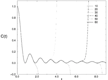
as t_→`. Note that in the long-time regime, C(t) oscillates with frequencyv54J, since the cosine function is squared. Our calculations ofC(t) involve the determination of the moments from the knowledge of the recurrants. From a given number of recurrants, one finds an equal number of moments. Thus, from those moments we construct a polyno-mial approximation forC(t), that is, a short-time expansion. Our approximate scheme, as outlined above, including the use of the ansatz for the recurrants, was tested with the known correlation function J₀(2Jt)2 for the disorderless case ofp51 (Ji5JB51.5). The results are shown in Fig. 2.

Note that the power-law ansatz, Eqs. ~22!–~24!, produces accurate results in the scale of the figure. The time region in

which the approximation is good is enlarged as more recur-rants from the ansatz are used. We find that we need at least 60 recurrants to obtain reasonable results.

IV. DISCUSSION AND CONCLUSIONS

The time-dependent correlation functions for several cases with disorder are displayed in Fig. 3, while the corre-sponding spectral densities are shown in Fig. 4. For p

50.0, we have the disorderless XY model with Ji5JA

51.0, while p51.0 corresponds to J_i5J_B51.5. Thus, the curves corresponding to the pure cases are the same, aside FIG. 2. Comparison between exact and approximate

longitudi-nal spin time-dependent correlation functions of theXYchain at the high-temperature limit. Shown are the exact results for the pure case p51, J0(3t)2, and those in which a given finite number of recurrants was used. Note the convergence as the number of recur-rants increases.

FIG. 3. Time-dependent spin-correlation function for the disor-deredXYchain at the high-temperature limit. The energy couplings are of typeJB51.5 with probabilityp, otherwise the couplings are

set toJA51.

FIG. 4. Spectral density of theXYmodel for several values ofp. The energies are in units ofJA, which serves to fix the horizontal

scale. The vertical scale is such that the area under each curve for

v>0 equalsp. Notice the large drops of the spectral density at

v54.0 and 6.0, which correspond to the pure cases p50.0 (Ji

5JA51.0) andp51.0 (Ji5JB51.5), respectively. Those drops are

(5)

from a time scale as one would expect. Thus, the correlation function for the stronger-coupling case oscillates with higher frequencies. In the limit t_→`, it oscillates with a single frequency, v54JB, which is the cutoff frequency for the

exact spectral density. In our calculations, where we trun-cated the continued fractions at the 60th level, where some information on the long-time dynamics was lost, the result is that the spectral densities for the casesp50.0 andp51.0 do not have the sharp edges as the exact functions do at their cutoff frequencies. In addition, the logarithmic divergence of the spectral density at v50 caused by the t21 _{behavior of} C(t) at large times is only hinted in our numerical results. There are also some minor spurious structures inF(v) that should be ignored. These pitfalls are all due to computational constraints that limited us to use only 60 recurrants for each case. Yet, our approximation still provides a reasonably good account on the effects of disorder in the model.

Asptakes on small values, the effect of disorder is to lift up the curvesC(t) above theJ₀(2t)2 result of the pure case Ji5JA51, as can be seen in Fig. 3. The lifting reaches a

maximum whenp50.5, that is, when the chain is most dis-ordered. Upon further increase ofp, the reverse takes place, that is, the curves forC(t) start to drop toward the pure case with stronger energy couplings J_B51.5. The plot of the

spectral density, Fig. 4, shows smooth curves for the cases with disorder, 0,p,1. Instead of having a sharp drop, the curves are smooth and show a tail that ends at the cutoff frequency of the stronger-coupling pure case p51.0. Thus, according to our results, there is also a cutoff frequency for the disordered cases, which is the same as the cutoff fre-quency of the pure stronger-coupling case, which is valid for all p, down top50.01. That is, the long-time dynamics of the disordered chain is dominated by the stronger couplings even if their concentration is very small. Based on our nu-merical evidence, we conjecture that such feature holds for all 0,p,1. It would be interesting to see how much of that asymptotic behavior could also appear in the cases where the coupling energies were drawn from a continuous distribu-tion. A similar behavior can be found in the density of states of one-electron systems in a binary alloy, where there ap-pears a low-energy tail, the so-called Lifshits tail, which is dominated by the rare large fluctuations of the potential.33

ACKNOWLEDGMENTS

This work was partially supported by CNPq, FAPEMIG, and PRONEX ~Brazilian agencies!.

*Electronic address: eugenia@fisica.ufmg.br

†_{Electronic address: jfj@if.uff.br}

1_{A.P. Young and H. Rieger, Phys. Rev. B}

53, 8486 ~1996!; A.P. Young,ibid.56, 11 691~1997!.

2_{J. Kotzler, H. Neuhaus-Steinmetz, A. Froese, and D. Gorlitz,}

Phys. Rev. Lett. 60, 647~1988!; R.W. Youngblood, G. Aeppli, J.D. Axe, and J.A. Griffin,ibid.49, 1724~1982!.

3_{B. Boechat, R.R. dos Santos, and M.A. Continentino, Phys. Rev.}

B 49, 6404 ~1994!; M.A. Continentino, B. Boechat, and R.R. dos Santos,ibid.50, 13 528~1994!.

4_{O. Derzhko and T. Krokhmalskii, Phys. Rev. B}₅₆_{, 11 659}_~₁₉₉₇_!_.

5_{J. Florencio and F.C. Sa Barreto, Phys. Rev. B}

60, 9555~1999!.

6_{B. Boechat, C. Cordeiro, J. Florencio, F.C. Sa Barreto, and O.F.}

de Alcantara Bonfim, Phys. Rev. B61, 14 327~2000!.

7_{E. Lieb, T. Schultz, and D. Mattis, Ann. Phys.} _~_N.Y._! ₁₆_{, 407}

~1961!.

8_{S. Katsura, Phys. Rev.}

127, 1508~1962!.

9_{Th. Niemeijer, Physica}_~_Amsterdam_!

36, 377~1967!; A very nice derivation of that result using a different method can be found in J. Hong, J. Korean Phys. Soc.25, 91~1992!.

10_{S. Katsura, T. Horiguchi, and M. Suzuki, Physica}_~_Amsterdam_!

46, 67~1970!.

11_{U. Brandt and K. Jacoby, Z. Phys. B}₂₅_{, 181}_~₁₉₇₆_!_.

12_{H.W. Capel and J.H.H. Perk, Physica A}₈₇_{, 211} _~₁₉₇₇_!_{; J.H.H.}

Perk and H.W. Capel,ibid.89, 265~1977!.

13_{J. Florencio and M.H. Lee, Phys. Rev. B}

35, 1835~1987!.

14_{M. Mohan, Phys. Rev. B}

21, 1264~1980!.

15_{S. Sen, Phys. Rev. B}₄₄_{, 7444}_~₁₉₉₁_!_.

16_{J. Stolze, V.S. Viswanath, and G. Mu¨ller, Z. Phys. B: Condens.}

Matter89, 45~1992!.

17_{S. Sen and T.D. Blersch, Physica A}

253, 178~1998!; S. Sen, Phys. Rev. B53, 5104~1996!.

18_{J. Stolze and M. Vogel, Phys. Rev. B}₆₁_{, 4026}_~₂₀₀₀_!_.

19_{M.H. Lee, Phys. Rev. Lett.}₄₉_{, 1072} _~₁₉₈₂_!_;₅₁_{, 1227} _~₁₉₈₃_!_;

Can. J. Phys.61, 428~1983!.

20_{M.H. Lee and J. Hong, Phys. Rev. Lett.}₄₈_{, 634}_~₁₉₈₂_!_.

21_{J. Florencio and M.H. Lee, Phys. Rev. A}₃₁_{, 3231}_~₁₉₈₅_!_.

22_{M.H. Lee, J. Hong, and J. Florencio, Phys. Scr., T} _T19_{, 498}

~1987!.

23_{J. Hong and M.H. Lee, Phys. Rev. Lett.}₇₀_{, 1972}_~₁₉₉₃_!_.

24_{M.H. Lee, Phys. Rev. E} ₆₁_{, 3571} _~₂₀₀₀_!_{; Phys. Rev. Lett.} ₈₇_,

250601~2001!; Physica A314, 583~2002!.

25_{I. Sawada, Phys. Rev. Lett.}

83, 1668 ~1999!; J. Kim and I. Sawada, Phys. Rev. E61, R2172~2000!.

26_{V. S. Viswanath and G. Mu¨ller,}

The Recursion Method: Applica-tion to Many-Body Dynamics, Lecture Notes in Physics Vol. 23

~Springer-Verlag, New York, 1994!.

27_{A.S.T. Pires, Helv. Phys. Acta}

61, 988~1988!.

28_{V.S. Viswanath and G. Mu¨ller, J. Appl. Phys.}

67, 5486~1990!.

29_{Z.X. Cai, S. Sen, and S.D. Mahanti, Phys. Rev. Lett.}

68, 1637

~1992!; S. Sen, S.D. Mahanti, and Z.X. Cai, Phys. Rev. B 43, 10 990~1991!.

30_{See, for example, U. Brandt and J. Stolze, Z. Phys. B: Condens.}

Matter64, 327~1986!; M. Bo¨hm and H. Leschke, J. Phys. A25, 1043~1992!.

31_{J.P. Boucher, M. Bakheit, M. Nechtshein, M. Villa, G. Bonera,}

and F. Borsa, Phys. Rev. B13, 4098~1976!; A. Lagendijk and E. Siegel, Solid State Commun.20, 709~1976!.

32_{The expressions for the basis vectors can be obtained from}

jfj@if.uff.br

33_{For more on Lifshits tails see, e.g., I. M. Lifshits, S. A. Gredeskul,}