SIMULATION OF MIXED MODELS IN AUGMENTED
BLOCK DESIGN
1Aladir Horacio Santos2*; Eduardo Bearzoti3; Daniel Furtado Ferreira3; João Luís da Silva Filho4
2
Depto. de Ciências Exatas - Faculdade de Filosofia - FUOM, C.P. 102 - CEP: 37570-000 - Formiga, MG.
3
Depto. de Ciências Exatas - UFLA, C.P. 37 - CEP: 37200-000 - Lavras, MG.
4
Depto. de Biologia - UFLA, C.P. 37 - CEP: 37200-000 - Lavras, MG. *Corresponding author <[email protected]>
ABSTRACT: The augmented block design is widely used in breeding programs, with non-replicated treatments generally being selection units, and replicated treatments being standard cultivars. Originally, an intrablock analysis (fixed model) was proposed. Although non-replicated treatments and/or blocks can be considered of random nature, mixed linear models could be used instead. This work evaluated such an approach, using computer simulation. Populations consisted of sets of randomly generated inbred lines. Molecular marker data were also simulated to allow the estimation of the genetic covariance matrix. Different conditions were considered, varying heritability and the coefficient b of Smith of soil heterogeneity. For each condition 100 simulations were performed, considering four linear models, varying respectively the nature of the effects of blocks and non-replicated treatments (fixed - F, or random - R): FF, FR, RF and RR. In relation to FF, the mixed models were more efficient under low to intermediate heritability and high b. Mixed models could improve inference in breeding programs using the augmented block design and the choice of the model should rely on the kind of selection. If this is truncated, the RF model should be preferred; if it is not, then the RR model would be more suitable.
Key words: augmented design, mixed model, molecular marker
SIMULAÇÃO DE MODELOS MISTOS NO DELINEAMENTO
EM BLOCOS AUMENTADO
RESUMO: O delineamento em blocos aumentados é amplamente utilizado em programas de melhoramento, geralmente com tratamentos não-repetidos correspondentes a unidades de seleção, e tratamentos repetidos sendo cultivares comerciais. Originalmente, uma análise intrablocos (modelo fixo) foi sugerida. No entanto, se os tratamentos não-repetidos e/ou blocos puderem ser considerados de natureza aleatória, modelos lineares mistos poderiam ser utilizados. Este estudo objetivou a avaliação de tal abordagem, utilizando simulação. Linhagens endogâmicas foram geradas aleatoriamente, bem como dados de marcação molecular, para estimar a matriz de covariâncias genéticas. Variaram-se a herdabilidade e o coeficiente b de heterogeneidade de solo de Smith; em cada condição, 100 simulações foram feitas, considerando 4 modelos lineares, variando respectivamente a natureza dos efeitos de bloco e de tratamentos não-repetidos (fixo – F, ou aleatório – A): FF, FA, AF e AA. Em relação ao modelo FF, os modelos mistos foram mais eficientes especialmente sob herdabilidade baixa a intermediária e alto b. Modelos mistos podem melhorar a inferência em programas de melhoramento utilizando o delineamento, e a escolha do modelo deve se basear no tipo de seleção. Se esta for truncada, o modelo AF deveria ser preferido; se não for, então o modelo AA é mais apropriado.
Palavras-chave: delineamento aumentado, modelo misto, marcador molecular
1Part of the MS Thesis of the first author, presented to UFLA - Lavras, MG. INTRODUCTION
The augmented designs were proposed by Federer (1956) as an alternative under low availability of genetic material for replication, and many treatments. They are a modification of straightforward designs, by adding treatments that appear only once in the experiment (herein designated simply as “treatments”) to the set of replicated treatments (“checks”). Among the augmented designs, the augmented block design is perhaps the most used, and inference has traditionally been made by means of an intrablock analysis (considering treatment and block effects fixed).
In plant breeding, this approach may be unsuitable, for in many cases such design is used with
treatments being selection units sampled from a population. Besides, recovery of information on treatments among blocks (interblock approach) can potentially improve the estimates, and this is achieved by regarding block effects as random. Genetic variances can be underestimated if the intrablock analysis is used in the augmented block design (Bearzoti, 1994). Therefore, the theory of mixed models (Henderson, 1984) could be used to take into account the randomness of the effects of treatments and/or blocks (Robinson, 1991). The effects of checks could be considered fixed in plant breeding, for they are generally standard released varieties.
designs straightforward. Scott & Milliken (1993) show an example of a SAS routine that yields the analysis of variance, hypothesis tests, intra and interblock estimation of treatment effects in augmented block designs. Boyle & Montgomery (1996) pointed out how intra and interblock approaches could be dealt using GLM and MIXED procedures of SAS software. Wolfinger et al. (1997), using such procedures, show routines to recover interblock and intervariety information when the nature of block and variety effects are actually random. Duarte (2000) presents a detailed study on the augmented block design, highlighting statistical issues and its use in plant breeding, showing many SAS routines to different alternatives of analysis of such designs, including the modeling of spatial residual dependence.
If treatment effects are regarded as random, e.g.
if they are sampled genetic materials, and if intergenotypic information is recovered, the predicted treatment means tend to show a decreased dispersion around the overall mean, in comparison to the dispersion of intrablock means. This trend is known as “shrinkage” effect, and reflects a more accurate distribution of genetic effects, if the assumption of randomness is correct (see, for instance, Duarte, 2000). The accuracy on estimating such distribution could be further improved if the matrix of covariances among genetic effects was known. In plant breeding, if treatments are genetic materials, such matrix could be constructed (apart, perhaps, from a constant corresponding to the genetic variance) using relationship information from molecular data, which can account for genetic similarities among treatments. This can be considered a simple way of marker-assisted selection, and relatively low-cost and fast generating markers like RAPD (random amplified polymorphic DNA) could be used.
There are reports in the literature on the use of a mixed model approach to analyze data of augmented block designs (Duarte, 2000; Federer, 1998), but its efficiency when covariances among treatments are not null and can be estimated has not yet been studied. Computer simulation is a powerful tool in such studies, for a wide range of conditions could be covered, in situations where an analytical approach has limitations.
This work aimed at the evaluation of the use of mixed model theory in augmented block designs, when treatments are selection units in a breeding program, and genetic covariances are estimated using molecular data.
MATERIAL AND METHODS
Augmented block designs were simulated using computational routines written with Delphi language, version 3. Treatments consisted of inbred lines of a fictitious diploid species with 200 independent genes controlling the trait of interest, and 100 marker loci were used to estimate the coefficients of genetic covariances among lines.
The frequency of the favorable allele in the population of lines of each gene was generated using a uniform distribution with parameters 0.2 and 0.8. A given line had a favorable allele with probability equal to the frequency of the corresponding gene. Genotypes regarding marker loci were simulated using the assumption that, for a given pair of lines, the number of marker loci with the same genotype had a binomial distribution with parameters r and s, where r was the number of markers (100) and s the genetic similarity in that pair of lines, considering the genes of the hypothetical trait. This assumption reflected basically the idea that similarities based on marker and trait loci are related.
The number n of lines were 50, 100 and 200. In each simulated condition, a different set of lines was used. The effects of each gene were generated as outcomes from an exponential distribution with parameter equal to 1, multiplied by -1 if the allele were not that favorable. Genotypic value of a given inbred line was calculated as the sum of the effects of all genes of that particular line. The variance among such genotypic values was the genetic variance across lines. Environmental variances were then obtained in such a way to yield heritability values (at the level of experimental plots) equal to 0.2, 0.5 and 0.8. This total environmental variance was partitioned into two components, associated to the variation within and among blocks, with magnitudes determined according to the value of the coefficient of soil heterogeneity of Smith (1938), represented by b, as suggested by Bearzoti (1997). Three values of b were evaluated: 0.1, 0.5 and 0.9.
The number of blocks was dependent on the number of lines, the former being 5% or 20% of the latter. Therefore, considering the 3 sample sizes (number of lines), the 3 values of the coefficient b, 2 amounts of blocks, and the 3 heritability values, 54 situations were analyzed. Each situation was simulated 100 times.
Every time a data set was generated, the following models were considered: 1) fixed effects of blocks and treatments (FF), corresponding to the intrablock analysis; 2) random block effects and fixed treatment effects (RF), corresponding to the analysis with recovery of interblock information; 3) fixed block effects and random treatment effects (FR), corresponding to the analysis with recovery of intergenotypic information; and 4) random effects of blocks and treatments (RR), recovering both interblock and intergenotypic information. The effects of the checks were always taken as fixed.
In order to compare estimates (or predictions) of treatment effects, θˆi to the corresponding genotypic values θi i = 1,2, ..., n), the following statistics were
calculated: mean square error (MSE); Spearman correlation, that reflects the accuracy on the ranking of lines, which is specially useful when selection is truncated; and “elite bias”, defined as the bias in the estimation of the percentage of treatments superior to the best check. The magnitude of such bias is relevant when selection is based in relation to standard cultivated varieties (non-truncated selection).
When variance components were considered unknown, they were estimated using restricted maximum likelihood (REML) and the EM algorithm (Dempster et al., 1977) associated to the mixed model equations of Henderson (1984). Convergence was considered to have been reached if, in a given iteration, the ratio(s) of the variance component of the factor (block or treatment) and residual variance component were different from that of the previous iteration in a magnitude no greater (in absolute value) than 10-8.
RESULTS AND DISCUSSION
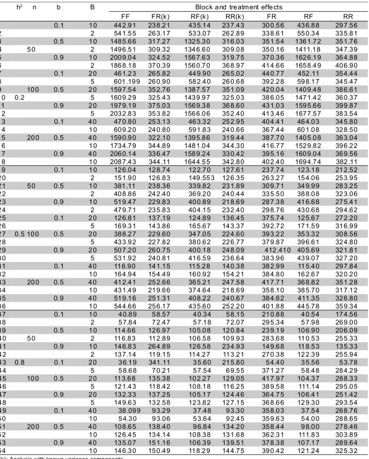
The MSE values of the estimated genetic effects, for all 54 configurations, are presented in Table 1. The RR(k) approach presented the smallest MSE values in 34 situations (53.1%). Most of the remaining 20 configurations were conditions of high heritability (h2 = 0.8). Among all situations with h2
= 0.8, only one presented the lowest MSE with RR(k) model, corresponding to n = 50 lines, b = 0.9 and number of blocks equal to 2. Three out of the 20 remaining configurations had h2 = 0.5, b = 0.1 and number of blocks equal to 0.2n. In such cases, however, the most precise approach was RF(k), which also assumes known variance components.
For the 17 situations with h2
= 0.8 and RR(k) approach not being the most precise, it can be seen that the MSE values of this model were more distant from the lowest MSE with b = 0.1, that is, when a higher fraction of environmental variance is due to the differences among blocks. Comparing, for example, situations 43 and 47 in Table 1, which have similar conditions, except for the value of b (0.1 and 0.9, respectively), in the former the RR(k) model had an MSE about six times the smallest, while in the latter this MSE was only 1.18 times the smallest. A single case of b different from 0.1, in which the RR(k) MSE was relatively high, was that with h2
= 0.8, n = 50, b = 0.9 and 10 blocks. In this configuration, the MSE of RR(k) was almost two times the smallest MSE.
The reasons why RR(k) did not show the smallest MSE, with high heritability, especially under relatively higher block effects, are not evident, since this approach theoretically yields the best linear unbiased predictions of random effects. However, when one
estimates variance components, predictors are no longer linear nor unbiased. A possible reason of reduction in precision might have been that the genetic variance taken as the parametric value was that among the actual 50, 100 or 200 lines, instead of the true population variance, considering all infinite possible inbred lines. The conditions under lower residual variation (higher h2) may have been more sensitive to this approximation. And, finally, even in the models where variance components were known, covariance coefficients were still unknown, and estimated via molecular information. So, it is not rigorously true that the RR(k) model should be the most precise ever.
The FR(k) approach had a trend very similar to that of RR(k), with regard MSE values, being less precise, in general. In 15 out of the 17 situations under high heritability, the RF(k) model had the smallest MSE. Therefore, there was a clear tendency of those approaches with known variance components to be most precise.
In an actual breeding program, variance components are generally (if not always) unknown, and so the comparison among FF, FR, RF and RR models is particularly relevant, especially to see whether the use of any mixed model (FR, RF or RR) shows any superiority to the intrablock analysis originally proposed by Federer (1956).
Considering only those models with unknown variance components in Table 1, the RR approach had the smallest MSE (higher precision) in most of the situations (53.7%), followed by RF (38.9%), similarly to the trends observed with the counterparts with known variance components. Again, most of the situations with RR not being the most precise model had high heritability (situations 37 to 54 of Table 1). However, in 4 of them heritability was equal to 0.5 and b was equal to 0.1 (situations 19, 25, 31 and 32), similarly to what happened with those models with known variance components. These results suggest that under low residual variation (high h2
and low b), prediction of treatment effects is less precise in models where such effects are random than those where they are fixed. There is, however, even in such circumstances, an increase in precision if interblock information is recovered.
Table 1 - Average values of the Mean Square Error (MSE) of the predictions of genetic effects of inbred lines across 100 simulations of augmented block designs with n = 50, 100 or 200 lines, heritability h2 equal to 0.5, 0.5 or 0.8,
coefficient of Smith b equal to 0.1, 0.5 or 0.9, and number of blocks given through 0.05n or 0.2n. Each column refers to a different model, varying the nature of the effect of blocks (1st letter) and of treatments (2nd letter): fixed (F) or random (R)1.
1(k): Analysis with known variance components.
h2 n b B Block a nd tre atment effe cts
Table 2 - Average values of the Spearman correlation among predictions and actual genetic effects of inbred lines across 100 simulations of augmented block designs with n = 50, 100 or 200 lines, heritability h2 equal to 0.5, 0.5 or 0.8,
coefficient of Smith b equal to 0.1, 0.5 or 0.9, and number of blocks given through 0.05n or 0.2n. Each column refers to a different model, varying the nature of the effect of blocks (1st letter) and of treatments (2nd letter): fixed (F) or random (R)1.
h2 n b B Block a nd tre atment effe cts
FF FR(k) RF(k) RR(k) FR RF RR 1 0.1 10 0.509 0.556 0.513 0.557 0.469 0.514 0.471 2 2 0.476 0.511 0.480 0.511 0.428 0.477 0.429 3 0.5 10 0.332 0.352 0.340 0.356 0.291 0.342 0.294 4 50 2 0.337 0.357 0.350 0.358 0.290 0.343 0.294 5 0.9 10 0.307 0.341 0.348 0.360 0.289 0.340 0.308 6 2 0.287 0.321 0.313 0.328 0.265 0.309 0.272 7 0.1 20 0.512 0.560 0.513 0.561 0.409 0.512 0.420 8 5 0.462 0.514 0.466 0.514 0.378 0.465 0.383 9 100 0.5 20 0.324 0.370 0.342 0.375 0.276 0.340 0.280 10 0.2 5 0.311 0.364 0.323 0.365 0.278 0.321 0.281 11 0.9 20 0.297 0.344 0.322 0.360 0.267 0.322 0.282 12 5 0.285 0.340 0.315 0.342 0.269 0.306 0.274 13 0.1 40 0.498 0.570 0.502 0.571 0.398 0.502 0.393 14 10 0.466 0.558 0.471 0.559 0.386 0.468 0.384 15 200 0.5 40 0.328 0.405 0.343 0.411 0.279 0.342 0.281 16 10 0.324 0.417 0.347 0.418 0.287 0.341 0.287 17 0.9 40 0.301 0.376 0.334 0.395 0.261 0.332 0.274 18 10 0.290 0.369 0.322 0.372 0.246 0.318 0.249 19 0.1 10 0.710 0.725 0.713 0.727 0.606 0.712 0.611 20 2 0.662 0.684 0.664 0.685 0.566 0.658 0.567 21 50 0.5 10 0.538 0.571 0.560 0.580 0.471 0.557 0.484 22 2 0.542 0.573 0.561 0.575 0.468 0.551 0.474 23 0.9 10 0.478 0.520 0.523 0.539 0.441 0.516 0.459 24 2 0.470 0.513 0.494 0.520 0.428 0.485 0.437 25 0.1 20 0.710 0.727 0.713 0.729 0.500 0.711 0.519 26 5 0.678 0.714 0.684 0.715 0.492 0.678 0.504 27 0.5 100 0.5 20 0.522 0.567 0.538 0.573 0.413 0.535 0.427 28 5 0.510 0.568 0.530 0.569 0.422 0.523 0.428 29 0.9 20 0.490 0.542 0.530 0.567 0.409 0.527 0.430 30 5 0.475 0.542 0.519 0.552 0.401 0.511 0.415 31 0.1 40 0.710 0.741 0.712 0.742 0.491 0.712 0.488 32 10 0.678 0.728 0.682 0.729 0.488 0.681 0.487 33 200 0.5 40 0.536 0.600 0.553 0.610 0.406 0.552 0.406 34 10 0.515 0.597 0.538 0.599 0.407 0.534 0.406 35 0.9 40 0.488 0.567 0.529 0.587 0.386 0.527 0.394 36 10 0.493 0.583 0.528 0.588 0.397 0.525 0.398 37 0.1 10 0.855 0.858 0.857 0.860 0.680 0.856 0.694 38 2 0.838 0.843 0.840 0.846 0.644 0.838 0.652 39 0.5 10 0.732 0.741 0.744 0.749 0.619 0.742 0.637 40 50 2 0.738 0.753 0.752 0.759 0.600 0.746 0.609 41 0.9 10 0.698 0.753 0.722 0.659 0.700 0.726 0.709 42 2 0.689 0.712 0.714 0.723 0.585 0.707 0.593 43 0.8 0.1 20 0.863 0.527 0.865 0.528 0.593 0.843 0.822 44 5 0.835 0.843 0.838 0.844 0.560 0.835 0.576 45 100 0.5 20 0.724 0.747 0.740 0.758 0.512 0.737 0.542 46 5 0.723 0.756 0.738 0.759 0.534 0.734 0.549 47 0.9 20 0.691 0.718 0.723 0.741 0.506 0.721 0.542 48 5 0.704 0.735 0.732 0.745 0.526 0.726 0.544 49 0.1 40 0.856 0.838 0.858 0.840 0.526 0.858 0.526 50 10 0.843 0.827 0.845 0.828 0.523 0.843 0.522 51 200 0.5 40 0.727 0.748 0.744 0.760 0.495 0.742 0.498 52 10 0.717 0.755 0.741 0.760 0.504 0.736 0.502 53 0.9 40 0.691 0.725 0.724 0.746 0.481 0.723 0.496 54 10 0.697 0.738 0.730 0.751 0.486 0.727 0.491
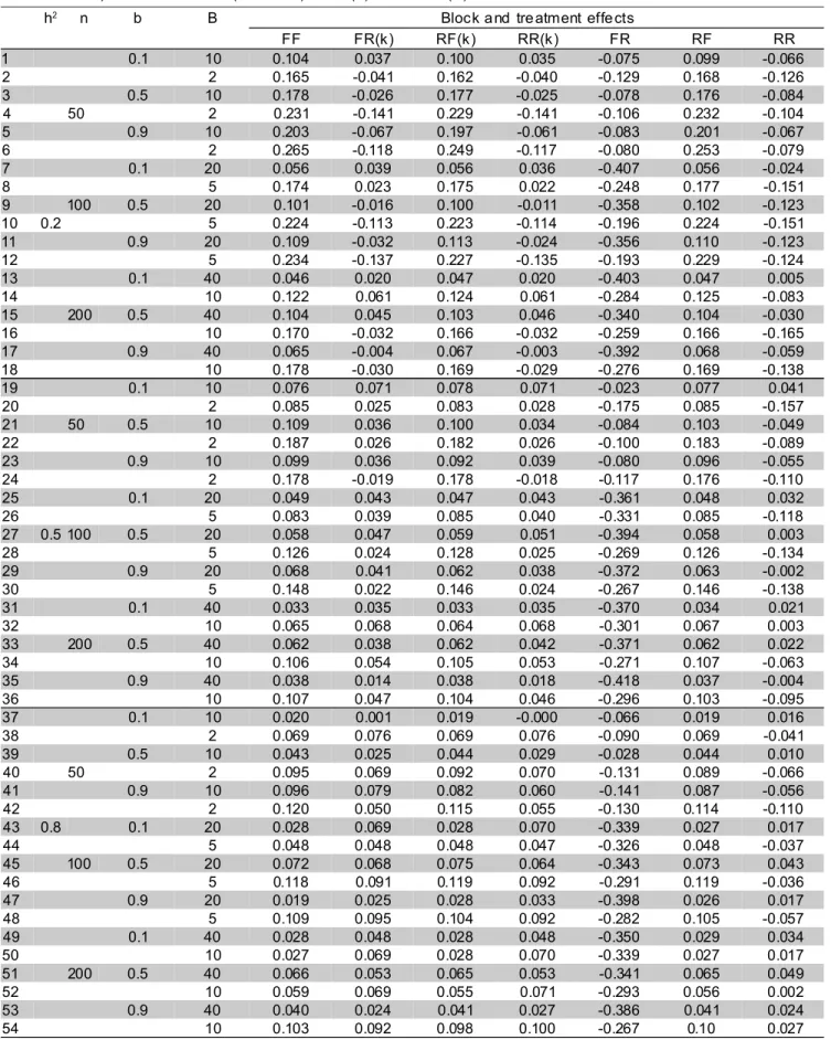
Table 3 - Average values of “elite bias” across 100 simulations of augmented block designs with n = 50, 100 or 200 lines, heritability h2 equal to 0.5, 0.5 or 0.8, coefficient of Smith b equal to 0.1, 0.5 or 0.9, and number of blocks given
through 0.05n or 0.2n. Each column refers to a different model, varying the nature of the effect of blocks (1st letter) and of treatments (2nd letter): fixed (F) or random (R)1.
1(k): Analysis with known variance components.
h2 n b B Block a nd tre atment effe cts
Focusing only on the approaches with unknown variance components, the RF model was generally superior to the others, with regard Spearman correlation (Table 2), having the highest values in 90.7% of the times (49 situations). In the remaining situations, the RF Spearman correlation was always close to the highest value observed (situations 20, 26, 38, 43 and 44). These results suggest that, for a wide range of conditions, if selection is truncated, interblock information should be recovered, the precision being at least comparable to the intrablock analysis. However, taking the randomness of the inbred lines into account seems unjustified, as well as the generation of molecular data, if one has to estimate variance components with the augmented block design.
In order to evidence those situations where recovery of interblock information is more noticeable, especially with truncated selection, one could take only those situations in Table 2 where the value of Spearman correlation of RF model was at least (say) 0.02 superior to that of FF model. There were 18 such cases, almost all with b equal to 0.9. Two exceptions were observed, with b equal to 0.5 (situations 9 and 16 of Table 2). This agrees with the fact that recovery of interblock information is more relevant when differences among blocks are small (high b), as pointed out by Duarte (2000).
If, however, in a breeding program, the selection is made in relation to a standard cultivated variety (non-truncated selection), then the “elite bias” is of particular interest (Table 3). Contrary to the trend observed with Spearman correlation, the RR(k) model was superior (smallest elite bias in absolute values) in a relatively low frequency (29.6%, or 31 situations). However, it must be noticed that such model showed an elite bias almost always quite close to the smallest observed. In the cases where this was not observed (situations 29, 32 and 35 of Table 3), the smallest value was observed with RR model, which is different from RR(k) only in the sense that variance components are estimated.
The RR approach presented the smallest elite bias (in absolute values) in most of the cases (85.2%). These results suggest that if selection is non-truncated, then recovery of both interblock and intergenotypic information is suitable, especially if genetic similarities are accounted for using molecular data. The efficiency of the recovery of intergenotypic information when selection is non-truncated is related to the shrinkage effect, typical to be observed with the random effects of mixed models, yielding a more accurate distribution of such effects, in relation to the ordinary least squares means (fixed model). Results in Tables 2 and 3 suggest that the choice of the model should be based on the type of selection that is to be practiced.
The superiority of RR model, in relation to elite bias, is more pronounced under intermediate to high values of b. For instance, confronting situations 2, 4 and 6 of Table 3, under the same conditions but the value of b, equal to 0.1, 0.5 and 0.9, it can be seen that the difference of the RR elite bias from that of RF increases from 0.04, in situation 2, to 0.13 and 0.17 in situations 4 and 6. Similar comparisons can be made, for example, taking situations 8, 10 and 12. With high heritability, such differences tend to diminish, but the same trend is observed varying the value of b (see, for example, elite bias of situations 50, 52 and 54, of RR and RF models). Anyway, this suggests that with high precision (high heritability and low b), non-truncated selection would also be effective considering treatment effects as fixed. The FR model was considerably poorer (Table 3), showing high (in absolute values) and negative elite biases, which would mean a high discard of elite lines.
The EM algorithm used in this study was extremely slow to converge, especially in the RR model, in which three variance components were to be estimated (residual, block and treatment). This suggests that this algorithm should be optimized to fit mixed models such as those of this study, or alternative numerical procedures should be investigated.
REFERENCES
BEARZOTI, E. Comparação entre métodos estatísticos na avaliação de clones de batata em um programa de melhoramento. Lavras, 1994. 128p. Dissertação (Mestrado) - Escola Superior de Agricultura de Lavras. BEARZOTI, E. Simulação recorrente assistida por marcadores moleculares
em espécies autogamas. Piracicaba, 1997. 230p. Tese (Doutorado) – Escola Superior de Agricultura “Luiz de Queiroz”, Universidade de São Paulo. BOYLE, C.R.; MONTGOMERY, R.D. An application of the augmented
randomized complete block design to poultry research. Poultry Science, v.75, p.601-607, 1996.
DEMPSTER, A.P.; LAIRD, N.M.; RUBIN, D.B. Maximum likelihood estimation from incomplete data via the EM algorithm (with discussion). Journal of the Royal Statistical Society. Series B, v.39, p.1-38, 1977.
DUARTE, J.B. Sobre o emprego e a análise estatística do delineamento em blocos aumentados no melhoramento genético vegetal. Piracicaba, 2000. 293p. Tese (Doutorado) - Escola Superior de Agricultura “Luiz de Queiroz”, Universidade de São Paulo.
FEDERER, W.T. Augmented (or hoonuiaku) designs. Hawaiian Planter’s Record, v.55, p.191–208, 1956.
FEDERER, W.T. Recovery of interblock, intergradient, and intervarietal information in incomplete block and lattice rectangle designed experiments. Biometrics, v.54, p.471-481, 1998.
HENDERSON, C.R. Applications of linear models in animal breeding. Ontario: Guelph, 1984.
ROBINSON, G.K. That BLUP is good thing: the estimation of random effects. Statistical Science, v.6, p.15-51, 1991.
SCOTT, R.A.; MILLIKEN, G.A. A SAS program for analyzing augmented randomized complete-block designs. Crop Science, v.33, p.865-867, 1993. SMITH, H.F. An empirical law describing heterogeneity in the yields of agricultural crops. Journal of Agricultural Science, v.28, p.1-23, 1938. WOLFINGER, R.D; FEDERER, W.T.; CORDERO-BRANA, O. Recovering information in augmented designs, using SAS PROC GLM and PROC MIXED. Agronomy Journal, v.89, p.856-859, 1997.