www.biogeosciences.net/13/3863/2016/ doi:10.5194/bg-13-3863-2016
© Author(s) 2016. CC Attribution 3.0 License.
Technical note: A bootstrapped LOESS regression approach for
comparing soil depth profiles
Aidan M. Keith, Peter A. Henrys, Rebecca L. Rowe, and Niall P. McNamara
Centre for Ecology & Hydrology, Lancaster Environment Centre, Library Avenue, Bailrigg, Lancaster, LA1 4AP, UK
Correspondence to:Aidan M. Keith ([email protected])
Received: 22 October 2015 – Published in Biogeosciences Discuss.: 4 December 2015 Revised: 25 May 2016 – Accepted: 8 June 2016 – Published: 6 July 2016
Abstract.Understanding the consequences of different land uses for the soil system is important to make better in-formed decisions based on sustainability. The ability to as-sess change in soil properties, throughout the soil profile, is a critical step in this process. We present an approach to ex-amine differences in soil depth profiles between land uses using bootstrapped LOESS regressions (BLRs). This non-parametric approach is data-driven, unconstrained by distri-butional model parameters and provides the ability to deter-mine significant effects of land use at specific locations down a soil profile. We demonstrate an example of the BLR ap-proach using data from a study examining the impacts of bioenergy land use change on soil organic carbon (SOC). While this straightforward non-parametric approach may be most useful in comparing SOC profiles between land uses, it can be applied to any soil property which has been measured at satisfactory resolution down the soil profile. It is hoped that further studies of land use and land management, based on new or existing data, can make use of this approach to examine differences in soil profiles.
1 Introduction
Understanding the consequences of different land uses for the soil system is important to better inform decisions based on sustainability (Foley et al., 2005; Haygarth and Ritz, 2009). The ability to assess change in soil properties affected by altered land use or management is therefore a critical step in this process. The greatest change is likely in the surface layers with factors such as tillage and plant inputs impacting the physical, chemical and biological properties of the soil. Many soil properties, however, will also be modified below
this depth, particularly as time since land use change (LUC) increases (Poeplau et al., 2011). It is therefore important that changes can be assessed below the topsoil and throughout the soil profile.
As a prime example, a number of studies, including global meta-analyses, have summarised the impacts of LUC on soil organic carbon (SOC) concentration and stocks (e.g. Guo and Gifford, 2002; Maquere et al., 2008; Laganière et al., 2010; Poeplau et al., 2011). SOC (sensu organic matter) is gener-ally concentrated in the top 30 cm of the soil and so LUC is generally expected to have the greatest impact on SOC in these upper layers (Lorenz and Lal, 2005; Laganière et al., 2010). Even within this surface soil, however, the magnitude and sometimes direction of the effects of LUC on SOC can depend on the depth that is being considered (Guo and Gif-ford, 2002; Popelau et al., 2011). It is also becoming more evident that, in addition to there being a large proportion of total SOC stocks resident in the subsoil, important C dynam-ics may also occur deeper in the soil (Jobbágy and Jackson, 2000; Lorenz and Lal, 2005).
greater contribution of recalcitrant litter and potential prim-ing down the soil profile (Fontaine et al., 2007). Altered land use or management may also impact the translocation of par-ticulate and dissolved organic C likely to occur down the soil profile via effects on leaching. Such mechanisms may pro-duce more complex relationships between soil depth and soil characteristics, and even discontinuous horizonation, rather than linear gradients.
2 Existing approaches to model soil depth profiles
Differences in SOC across transitions and soil depth pro-files can be tested with both land use and depth included as fixed factors in an interaction model, and appropriate random terms to account for non-independence of depth increments within the same core and/or plots. There are, however, var-ious potential modelling approaches that have been used to examine soil depth profiles including, for example, modified exponential decay (Maquere et al., 2008), depth distribution functions which utilise multiple regression (Indorante et al., 2013) and spline functions (Bishop et al., 1999; Malone et al., 2009; Wendt and Hauser, 2013). Another common method for non-linear modelling is the use of generalised additive models (Hastie and Tibshirani, 1990).
Recent work modelling depth profiles has focussed on de-riving parametric non-linear relationships between soil depth and the response of interest. Maquere et al. (2008) adopt a parametric form with modified exponential decay, whereas Myers et al. (2011) use an approach based on asymmetric peak functions. Whilst capturing the non-linear form of the soil depth profile, neither exponential decay nor polynomial methods adequately handle the associated uncertainty and hence confidence intervals, with the method in Maquere et al. (2008) assuming atdistribution and the method in Myers et al. (2011) failing to produce confidence envelopes at all. Regression-based approaches similar to the popular GAM method have also been adopted using multiple covariates to account for any non-linearity (Indorante et al., 2013) and fit-ting cubic splines directly (Wendt and Hauser, 2013). How-ever, the multiple regression approach assumed a normal dis-tribution of the response variables, which is often not re-alised, and the cubic spline method presented by Wendt and Hauser does not provide any measure of uncertainty.
Non-linear relationships between SOC and soil depth across LUC transitions can also be incorporated by the in-clusion of flexible splines (Bishop et al., 1999; Wood, 2003; Malone et al., 2009). In particular, the use of equal-area smoothing splines has long been considered as a beneficial approach to alleviate issues of modelling continuous soil depth functions using increment or horizon data (Bishop et al., 1999) and recent work has utilised the approach in the large-scale mapping of soil properties (Malone et al., 2009; Odgers et al., 2012; Adhikari et al., 2014). Equal-area spline functions consist of locally fitted quadratic functions tied
together with knots at horizon boundaries (Malone et al., 2009), and the areas under/over the fitted curve optimised for equality in each horizon (Bishop et al., 1999). Confidence intervals and significance tests are, however, based upon the assumption that the response variable is drawn from the ex-ponential family of distributions and inference is very sensi-tive to this assumption. Malone et al. (2009), in their study mapping continuous depth functions of SOC and water stor-age, highlighted the need for better estimation of uncertainty in such model outputs, suggesting the use of simulation and re-sampling approaches.
Simulation and re-sampling techniques avoid the necessity to assume a distributional form for the response variable in order to obtain confidence intervals and test hypotheses. Such approaches are rarely used to investigate soil depth relation-ships despite the often flawed assumptions made by the more commonly applied methods. Clifford et al. (2014) adopted a simulation routine from a master database to impute missing values, and this clearly demonstrated another strength of the simulation approach, though they did not apply the method directly to test specific hypotheses relating to changes along the soil profile.
We sought to develop an approach which (1) would be able to compare and test for significant differences between potentially non-linear depth profiles of land uses (or across land use transitions), (2) did not need to meet any parametric distribution assumptions given that individual datapoints in soil datasets are typically non-independent (i.e. vertically or horizontally nested measurements) and (3) would be gener-ally applicable regardless of specific contexts of land use and soil type. Below, we describe the resulting non-parametric approach and provide an example comparing SOC depth pro-files across a land use transition.
3 A bootstrapped LOESS regression (BLR) approach
The developed approach combines bootstrapped resampling of data with local least-squares-based polynomial smooth-ing (LOESS) regression. Consequently, this non-parametric method benefits from being data-driven and unconstrained by distributional form or rigid model parameterisation. Like spline approaches (Malone et al., 2009; Wendt and Hauser, 2013), it does not assume constant values for soil layers or horizons. Such a non-parametric approach is highly suitable where data are non-independent. This is particularly appli-cable in soil profiles where measurements made in depth increments down a soil profile may be correlated and even more relevant where data are cumulative (e.g. cumulative C stocks). It is also appropriate where soil cores have been sam-pled using a nested spatial design with multiple cores taken from within plots.
res-olution satisfactory for the purposes of an assessment. The vertical sampling resolution is not limited to any specific depth interval (e.g. 10 cm increments) but clearly a greater, and regular, resolution provides more detailed information on potential differences and their specific location in the soil profile. Low sample sizes will affect the amount of smooth-ing that can be done by the LOESS algorithm. As the al-gorithm fits polynomial regressions within local neighbour-hoods, the definition and size of the neighbourhood deter-mines the smoothness and sensitivity of the fitted regression line. Typically a minimum of three observations per neigh-bourhood would be required.
The initial dataset comprises all data for the soil variable of interest from the two land uses (LU1∪LU2=LUALL)which are to be compared, with the associated depth and/or soil mass as reference. A subset is then created containing only data from the “second” land use (LU2). In theory, it does not matter which of the land uses are subsetted for LU2but one may be more intuitive given the direction of a specific land use transition. It is also useful to plot the data to de-termine whether the datasets contain outliers that may need to be excluded before bootstrapping to prevent skewing the LOESS regression. For cumulative mass-based data, if dat-apoints from the bottom depths of either LU1or LU2are at distinctly greater cumulative masses than others, these could also be trimmed so that the comparison is made to the same approximate lower bounds of the reference. Using a large number of bootstrap samples, however, should negate the need for extensive data cleansing prior to analysis.
The combined data (LUALL)are re-sampled by bootstrap with replacement, with the number of datapoints resampled equal to the number of datapoints in LU2. This is repeated n=1000 times. Each bootstrapped set of data is then mod-elled using LOESS regression, and these regressions are used to generate 95 % confidence intervals around a modelled soil depth profile by taking pointwise percentiles at each depth. As each subsample is taken from the union of the two land uses, this confidence interval (or confidence envelope) rep-resents the null hypothesis that there is no difference be-tween the LU1 and LU2. The data from only LU2 are then modelled using LOESS regression; if the modelled line for the LU2 profile sits outside the confidence envelope of the null hypothesis it can be inferred that the soil variable is sig-nificantly different between LU1 and LU2 at that particular point in the profile. OverallP values for the difference be-tween depth profiles can be obtained by taking normalised test statistics across the full set of bootstrap samples and tak-ing the percentile of these values correspondtak-ing to the same statistic obtained from the LU2 data. This is a similar ap-proach to that adopted in the spatial statistics literature when analysingKfunctions under resampling as demonstrated in Diggle et al. (2007) and Henrys and Brown (2009) for exam-ple.
This relatively straightforward non-parametric method may be most useful in comparing SOC profiles between land
uses, but it can be applied to any soil property which has been measured at satisfactory resolution down the soil pro-file. Many of these other properties measured in soil (e.g. bulk density, pH, root biomass) can vary in a non-linear fash-ion down the soil profile, with potential horizonatfash-ion. The ef-fects of land use change are typically examined using either a paired-site or chronosequence approach. These assume that each paired or chronosequence site only differs in their age or, for example, time since disturbance and have comparable biotic and abiotic histories (Laganière et al., 2010). While this BLR method benefits from being unconstrained by sumptions of parametric methods, it must still satisfy the as-sumptions of the paired-site and chronosequence approaches, particularly if space-for-time substitution is used (Indorante et al., 2013). Here, we provide an example comparing SOC depth profiles between land uses. The approach is, however, not limited to comparing soil depth profiles between land uses. It could also be usefully adopted to examine, for exam-ple, depth functions in lake systems or to compare temporal trajectories in soil metrics between experimental treatments.
4 Applying a BLR approach – an example of bioenergy land use change
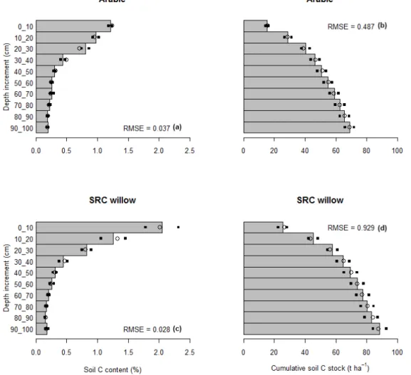
Figure 1.Soil carbon concentration(a, c)and cumulative carbon stock(b, d)of arable(a, b)and SRC willow(c, d)land uses in 10 cm depth increments to 1 m. Bars represent observed means, squares the standard error of observed means, and open circles the modelled means. Root mean square error (RMSE) calculated for the depth profile using means of observed and modelled data from the 10 depth increments.
SOC concentration, as these data are not directly influenced by core volume and apparent bulk density.
There was generally a good fit between observed and mod-elled data, with all modmod-elled means well within a standard error of the observed means in each depth increment, and the majority very close to the actual observed mean (Fig. 1). The poorest fits appeared to be for SOC concentration around the plough layer of the arable land use (20–40 cm; Fig. 1a) and in the upper layers of the SRC willow land use (0–20 cm; Fig. 1c). The RMSE values for the depth profiles were 0.037, 0.487, 0.028 and 0.929 for arable SOC concentration, arable SOC stock, SRC willow SOC concentration and SRC willow SOC stock, respectively.
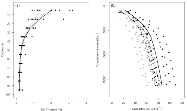
Individual datapoints for each land use, the confidence en-velope of the null hypothesis and the modelled profile for the SRC willow were plotted following BLR (Fig. 2). Where the modelled line sits outside the confidence envelope it can be inferred whether there are significant effects of land use in the soil profile, at either a particular depth or referenced soil mass. In Fig. 2a, the SOC concentration is significantly
greater under SRC willow compared with arable at 10 and 20 cm, where the modelled line sits to the right of the con-fidence envelope. The modelled line sits within the confi-dence envelope between 40 and 100 cm, so there is no sig-nificant difference (Fig. 2a). Nevertheless, the two depth pro-files are significantly different overall (P <0.01). The depth profile of SOC concentration is reflected in the cumulative SOC stock profile, with the modelled line for SRC willow moving further from the confidence envelope up to approx-imately 5000 t ha−1 (Fig. 2b). The difference in cumulative SOC stock between arable and SRC willow is maintained to 100 cm and, consequently, is significantly different down the whole soil profile (P <0.01; Fig. 2b).
5 Conclusions
Figure 2.Difference in profiles of(a)soil C concentration as a function of sampling depth and(b)cumulative soil C stock as a function of soil mass. Depth represents values of samples from 10 cm increments. Grey and black symbols represent SRC willow and arable datapoints, respectively. Dashed lines represent upper and lower bounds of 95 % confidence intervals from bootstrapped (n=1000) LOESS regressions of combined arable and SRC willow data; solid lines represent LOESS regression of percent C and cumulative soil C in SRC willow only. If this line sits outside the confidence interval, it can be inferred that arable and SRC willow are significantly different.
LOESS regression. The development of this approach was driven by a need for a flexible method which could com-pare potential non-linear relationships between land uses (or across land use transitions) and would not be constrained to specific contexts. While there are several other methods which can be used to model non-linear relationships in soil depth profiles, the BLR approach is flexible because it is data-driven and does not need to meet any distributional as-sumptions. The confidence envelopes obtained are robust to miss-specification of the error distribution and provide clear inspection of significant differences across the full depth pro-file. There can be issues of model fit when profiles are discon-tinuous or change abruptly. This is not exclusive to the BLR approach though and it also affects equal-area spline mod-els (see Odgers et al., 2012). It has been proposed that the use of pseudo-horizons may help towards overcoming this challenge (Malone et al., 2009; Odgers et al., 2012). We ac-knowledge that in some circumstances the equal area spline functions are a viable alternative to LOESS regression for producing a fitted profile. This could, however, easily be in-corporated into the non-parametric estimation and bootstrap-ping framework that we present here.
Sampling to depth and increasing the resolution of depth increments can provide useful profiles or “fingerprints” of soil properties under different land uses and soil types. In particular, assessment of SOC to depth, and determining the response of SOC to land use change (LUC) or land
manage-ment change is essential to understand the sustainability of different soil use options. This may be particularly important for land-use transitions to perennial crops, which have deeper and more permanent rooting systems that may influence the C balance deeper in the subsoil via priming of decomposi-tion, C stabilisation or translocation. The BLR approach can be, however, applied to any soil property of interest giving the ability to assess land use effects at any point down the soil profile. Being data-driven and flexible, it is hoped that further studies of land use and land management, based on new or existing data, can make use of this approach to exam-ine differences in soil profiles.
6 Data availability
Example code to demonstrate the BLR approach using these data is available via doi:10/f3jp5d (Keith et al., 2015).
Acknowledgements. This work was supported by the ELUM (Ecosystem Land Use Modelling & Soil Carbon GHG Flux Trial) project, which was commissioned and funded by the Energy Technologies Institute (ETI).
Edited by: E. Veldkamp
References
Adhikari, K., Hartemink, A. E., Minasny, B., Bou Kheir, R., Greve, M. B., and Greve, M. H.: Digital mapping of soil organic car-bon contents and stocks in Denmark, PLoS One 9, e105519, doi:10.1371/journal.pone.0105519, 2014.
Bishop, T. F. A., McBratney, A. B., and Laslett, G. M.: Modelling soil attribute depth functions with equal-area quadratic smooth-ing splines, Geoderma, 91, 27–45, 1999.
Clifford, D., Dobbie, M. J., and Searle, R.: Non-parametric imputa-tion of properties for soil profiles with sparse observaimputa-tions, Geo-derma, 232–234, 10–18, 2014.
Diggle, P. J., Gómez-Rubio, V., Brown, P. E., Chetwynd, A. G., and Gooding, S.: Second-Order Analysis of Inhomogeneous Spatial Point Processes Using Case–Control Data, Biometrics, 63, 550– 557, 2007.
Foley, J. A., DeFries, R., Asner, G. P., Barford, C., Bonan, G., Car-penter, S. R., Chapin, F. S., Coe, M. T., Daily, G. C., Gibbs, H. K., Helkowksi, J. H., Holloway, T., Howard, E. A., Kucharik, C. J., Monfreda, C., Patz, J. A., Prentice, I. C., Ramankutty, N., and Snyder, P. K.: Global consequences of land use, Science, 309, 570–574, 2005.
Fontaine, S., Barot, S., Barre, P., Bdioui, N., Mary, B., and Rumpel, C.: Stability of organic carbon in deep soil layers controlled by fresh carbon supply, Nature, 450, 277–280, 2007.
Gál, A., Vyn, T. J., Michéli, E., Kladivko, E. J., and McFee, W. W.: Soil carbon and nitrogen accumulation with long-term no-till versus mouldboard plowing overestimated with no-tilled-zone sampling depths, Soil Till. Res., 96, 42–51, 2007.
Gifford, R. M. and Roderick, M. L.: Soil carbon stocks and bulk density: spatial or cumulative mass coordinates as a basis of ex-pression?, Glob. Change Biol., 9, 1507–1514, 2003.
Guo, L. B. and Gifford, R. M.: Soil carbon stocks and land use change: a meta analysis, Glob. Change Biol., 8, 345–360, 2002. Hastie, T. J. and Tibshirani, R. J.: Generalized additive models (Vol.
43), CRC Press, 1990.
Haygarth, P. M. and Ritz, K.: The future of soils and land use in the UK: Soil systems for the provision of land-based ecosystem services, Land Use Policy, 26S, S187–S197, 2009.
Henrys, P. A. and Brown, P. E.: Inference for clustered inhomoge-neous spatial point processes, Biometrics, 65, 423–430, 2009. Indorante, S. J., Kabrick, J. M., Lee, B. D., and Maatta, J. M.:
Quan-tifying Soil Profile Change Caused by Land Use in Central Mis-souri Loess Hillslopes, Soil Sci. Soc. Am. J., 78, 225–237, 2013. Jobbágy, E. G. and Jackson, R. B.: The vertical distribution of soil organic carbon and its relation to climate and vegetation, Ecol. Appl., 10, 423–436, 2000.
Keith, A. M., Henrys, P. A., Rowe, R. L., and McNamara, N. P.: Bootstrapped local regression (LOESS) for soil depth pro-file comparison, NERC Environmental Information Data Centre, doi:10.5285/d4f92cd8-43e8-49e4-8f9e-efcc0e3b2478, 2015. Laganière, J., Angers, D. A., and Parè, D.: Carbon accumulation
in agricultural soils after afforestation: a meta-analysis, Glob. Change Biol., 16, 439–453, 2010.
Lorenz, K. and Lal, R.: The depth distribution of soil organic carbon in relation to land use and management and the potential of car-bon sequestration in subsoil horizons, Adv. Agron., 88, 35–66, 2005.
Malone, B. P., McBratney, A. B., Minasny, B., and Laslett, G. M.: Mapping continuous depth functions of soil carbon storage and available water capacity, Geoderma, 154, 138–152, 2009. Maquere, V., Laclau, J. P., Bernoux, M., Saint-Andre, L.,
Gonçalves, J. L. M., Cerri, C. C., Piccolo, M. C., and Ranger, J.: Influence of land use (savanna, pasture,Eucalyptusplantations) on soil carbon and nitrogen stocks in Brazil, Eur. J. Soil Sci., 59, 863–877, 2008.
Myers, D. B., Kitchen, N. R., Sudduth, K. A., Miles, R. J., Sadler, E. J., and Grunwald, S.: Peak functions for modelling high reso-lution soil profile data, Geoderma, 166, 74–83, 2011.
Odgers, N. P., Libohova, Z., and Thompson, J. A.: Equal-area spline functions applied to a legacy soil database to create weighed-means maps of soil organic carbon at a continental scale, Geo-derma 189–190, 153–163, 2012.
Poeplau, C., Don, A., Vesterdal, L., Leifeld, J., Van Wesemael, B., Schumacher, J., and Gensior, A.: Temporal dynamics of soil or-ganic carbon after land-use change in the temperate zone – car-bon response functions as a model approach, Glob. Change Biol., 17, 2415–2427, 2011.
R Core Team: R: A language and environment for statistical com-puting, R Foundation for Statistical Comcom-puting, Vienna, Austria, http://www.R-project.org, 2015.
Rowe, R. L., Keith, A. M., Elias, D., Dondini, M., Smith, P., Oxley, J., and McNamara, N. P.: Initial soil C and land-use history determine soil C sequestration under perennial bioen-ergy crops, Glob. Change Biol. Bioenbioen-ergy, Early View Online, doi:10.1111/gcbb.12311, 2016.
Wendt, J. W. and Hauser, S.: An equivalent soil mass procedure for monitoring soil organic carbon in multiple soil layers, Eur. J. Soil Sci., 64, 58–65, 2013.