www.earth-syst-sci-data.net/2/157/2010/ doi:10.5194/essd-2-157-2010
©Author(s) 2010. CC Attribution 3.0 License. Open
Access
Science
Data
Measuring hydrodynamics and sediment transport
processes in the Dee Estuary
R. Bola ˜nos and A. Souza
National Oceanography Centre, Joseph Proudman Building, 6 Brownlow Street, Liverpool, L3 5DA, UK
Received: 15 February 2010 – Published in Earth Syst. Sci. Data Discuss.: 3 March 2010 Revised: 13 May 2010 – Accepted: 20 May 2010 – Published: 14 June 2010
Abstract. The capability of monitoring and prediction in the marine environment provides information that may allow sustainable development of coastal and offshore regions. Therefore, the continuous measurement of environmental processes becomes an important source of information. The present paper shows data collected during 6 years, and in particular during 2008, in the Dee Estuary. The aim of the data collection is to improve the observations of the mobile sediments in coastal areas and its forcing hydrodynamics and turbulence. Data includes information from the deployment of instrumented rigs measuring sediment in suspension, currents, waves, sea level, sediment size and bedforms as well as cruise work including grab sampling, CTD profiles and side-scan sonar. The data cover flood and ebb tides during spring and neap periods with moderate and mild wave events, thus, having a good coverage of the processes needed to improve knowledge of sediment transport and the parameterizations used in numerical modelling. The data, in raw and treated, are being banked at BODC (British Oceanographic Data Centre, http://www.bodc.ac.uk/) which is the formal British organization for looking after and distributing data concerning the marine environment.
1 Introduction
Coastal areas support many human activities of economic, industrial and leisure importance. Moreover, they represent a very important habitat for many marine and bird species. In order to manage properly such areas, knowledge of the physi-cal, biological and chemical processes is necessary and there-fore the observation, quantification and simulation of such processes are very important. Coastal ecosystems are experi-encing changes affecting the dynamic boundary between the land and the sea. Coastal waves and currents are highly vari-able and can have a significant impact on human activities and structures. Therefore, the continuous research and im-provement of environmental monitoring has become a vital issue for the safety and well-being of coastal society. The ca-pability of monitoring and prediction in the marine environ-ment provides information that may allow sustainable devel-opment of coastal and offshore regions (Pinardi and Woods, 2002; GOOS, 2003).
Correspondence to:R. Bola˜nos ([email protected])
In recent years, the scientific community has been pay-ing more attention to several aspects of wave-current-bed-sediment interaction. Mastenbroek et al. (1993) showed how a wave-dependent bottom drag coefficient improved the re-sults of a 2-D storm surge model in the North Sea. Baumert et al. (2000), Souza et al. (2001) and Bola˜nos et al. (2005), using a coupled wave-tidal-circulation model, showed the relevance of wave action over the stress at the sea bed and thereby the erosion and suspension of particulate matter. Brown and Wolf (2009) improved storm surge modelling by considering a wave dependent surface stress. Thus, si-multaneous measurements of such processes are necessary, though not common, to understand and improve its mod-elling. There is a pressing need for improved observations of the mobile sediments in coastal areas in order to upgrade modelling systems, ultimately allowing the appropriate man-agement of nearshore and estuarine areas that are under in-creasing pressure.
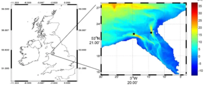
Figure 1.Location of the Dee Estuary in the Irish Sea. Right figure shows the Dee bathymetry and location of rigs at the Welsh (West) and Hilbre (East) channels. Colour scale shows water depth in me-ters, negative values represent height above mean sea level.
sediments, in combined waves and currents; and to make a critical assessment of the extent to which the predictive capa-bilities related to sand transport remain valid in a mixed sed-iment environment. The data set represent a unique source of information due to the simultaneous measurements of the processes involved in sediment transport.
The Dee (Moore et al., 2009; Simpson et al., 2004) is a macrotidal estuary characterized by the presence of waves at its outer margins, strong tidal flows in its channels, and a mixed seabed usually muddy sands or sandy muds. The over-all transport direction, in or out of the main outer channels of the estuary, is probably grain-size dependent. The Dee is, thus, a conveniently located “natural laboratory”.
The present paper shows data collected during 6 years, and in particular during 2008. First a detailed description of the Dee Estuary is given. Then details of rigs and instrumen-tations deployed are discussed together with an overview of the data and the environmental conditions during the record-ing period. Comprehensive data of the Dee Experiment are also summarized in Sect. 6. Finally the conclusions are pre-sented outlining the key aspects that can be addressed with this data set.
2 The Dee Estuary
The Dee is a macrotidal, funnel-shaped estuary situated in the eastern Irish Sea (Fig. 1). It has a length of about 30 km, with a maximum width of 8.5 km at the mouth of the estu-ary. The average tidal prism in the Dee is 4×10⁸m3, annual mean river discharge is only of 31 m3/s (with peak flows of the order of 300 m3/s) making the Dee a tidal dominated es-tuary. Tidal range during mean spring at Hilbre Island is in the order of 10 m. A tidal bore has been reported to occur in the canalised upper part of the estuary (Simpson et al., 2004). Moore et al. (2009) report a sediment import into the estuary, but it is suggested that the Dee could be reaching a morphological equilibrium and that the rate of accretion may decrease in the future. The main channel bifurcates 12 km seaward from the canalised river at the head of the estuary,
resulting in two deep channels extending into Liverpool Bay. The Dee Estuary presents a mixture of sediments containing a range of non-cohesive and cohesive sediments (Baas, J. H.: Bottom sediment characteristics at (mini)STABLE sites, per-sonal communication, 4th FORMOST Meeting, 2009) and, therefore, the threshold of motion of the bed might be a com-plex process dependent on several conditions. The estuary is a major wildlife area and is one of the most important estuar-ies in Britain and amongst the most important in Europe for its populations of waders and wildfowl. The two shorelines of the estuary show a marked contrast between the industri-alised usage of the coastal belt in Wales and residential and recreational usage in England. The estuary has been subject of several man made modifications such as canalisations and training wall causing siltation and accretion on the eastern shore and colonisation of some areas by saltmarsh.
The estuary contains extensive areas of intertidal sand and mudflats (Hutchinson, 1994; Hutchinson and Prandle, 1994) which support a variable but characteristic benthic fauna de-pending on the nature of the substrate. Large areas of salt-marsh also occur at its head and along part of its north-eastern shore. The three sandstone islands which comprise the Hilbre Island complex represent the only natural hard rock coast within the estuary.
3 Instrumentation and deployments
The Dee Estuary has been subject of study and measurements by the Proudman Oceanographic Laboratory (POL, renamed the National Oceanography Centre from 1 April 2010) since 2004 when deployment of rigs and cruises in the area started to take place. Recently, within the NERC funded FORMOST (Field observation and modelling of the sed-iment triad) project (http://www.pol.ac.uk/home/research/ formost/), measurements were carried out during 2008 and 2009.
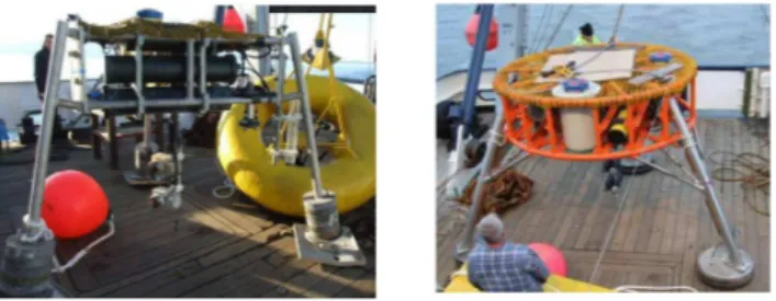
The measurement program in the Dee during 2008 con-sisted of the deployment of 2 recent versions of STABLE (Sediment Transport and Boundary Layer Equipment) rigs. STABLE is a platform to study near-bed turbulent currents and associated sediment-dynamics. The biggest and most complex structure designed and built by the Mechanical Engineering group at POL is the STABLE-III equipment (Fig. 2). STABLE-III is the third generation of this appa-ratus which was conceived originally in 1981. It measures the interactions between turbulent currents and sediments at the sea-bed. It is a tripod standing about 2.5 m high and the feet occupy a circle about 3.5 m in diameter: it weighs about 2500 kg (Williams et al., 2003). Mini-STABLE (Fig. 2) is a smaller version of STABLE-III. STABLE-III and mini-STABLE were deployed in the Hilbre Channel and Welsh Channel respectively (Fig. 1).
Figure 2.Mini-STABLE (left) and STABLE-III (right) during the deployment manoeuvres on the Prince Madog.
(12 February 2008) in the Welsh channel, and STABLE-III two days later in Hilbre channel. Rigs were equipped with different instruments to measure currents, waves, con-centration of sediment in suspension, sediment size, salin-ity and temperature. Instruments used were ADVs (Acous-tic Doppler Velocimeter, Sontek ADVocean 5 MHz) able to rapidly and accurately sample 3-D current component in a small sampling volume by using the pulse-coherent tech-nique.
ABS (Acoustic Backscatter System, built at POL) mea-sures the strength of backscatter signal that can be inverted to obtain concentration and size of particles in suspension in the water column. The use of acoustic backscatter (ABS) techniques to measure suspended sediment dates back to the 1980s (Crawford and Hay, 1993; Young et al., 1982; Thorne and Campbell, 1992).
LISST (Laser In Situ Scattering and Transmissometry, from Sequoia) designed to measure particle size based on the principle of laser diffraction. The standard processing software supplied with the LISST computes the volume con-centration in units of microlitres per litre (ul/l). The LISST laser optics must be checked on a regular basis to ensure that they remain properly aligned (Styles, 2006) and background scatter calibration must be also performed.
ADCP (Acoustic Doppler Current Profiler, from Teledyne RD Instruments), which measures the velocity of water using a physical principle similar to the ADVs. Traditionaly ADCP have been used to study current profiles with resolution of the order of 0.5 m but nowadays ADCP instruments can be used for resolution of up to 1 cm allowing the study of turbulence and sediments transport.
The rigs also contained ripple profilers, mini-STABLE had a line scan ripple profiler and STABLE-III a 3-D scanner which is a line scan ripple profiler that rotates to provide an area coverage. The transducer allows to find the bed position within a spatial resolution of about 5 mm and with an error of 0.01 m (Williams et al., 2004, 2005).
In order to measure turbidity (suspended particulate mat-ter) a series of optical backscatter sensors (OBS, from Camp-bell Scientific, Inc.) were installed to the ADVs. OBS mea-sure turbidity on NTU units, the instruments were set to a low turbidity range. Serial numbers of the OBS are T8193,
T8194 and T8195 with the calibration formula as
2.5×10−6X2+0.0946201X+0.061581,
2.4×10−6X2+0.094505X−0.0493607 and
2.4×10−6X2+0.0916872X+0.0881808 respectively.
Pre-deployment instrument operations consisted of typi-cal servicing, typi-calibration and testing of instruments. Syn-chronization of clocks were performed and instruments were set to start the recording at 06:00 GMT on 12 February 2008 for mini-STABLE and 06:00 GMT on 14 February 2008 for STABLE-III.
In order to deploy and recover the rigs, an oceanographic research vessel (Prince Madog) was used. The deployment and recovery periods were used also to perform CTD profile and LISST station, grab sampling and side-scan sonar tran-sects.
3.1 Welsh channel deployment
All parts for mini-STABLE were transported to Menai Bridge, UK, and loaded onto the Prince Madog and then de-ployed in the Welsh channel. Instruments on the rig were 2 ADVs, 1 ABS, a line scan ripple profiler, a sediment trap, a LISST and ADCP. Unfortunately the ADCP and ABS were damaged and data were lost. Figure 2 shows the rig before the deployment manoeuvres. Table 1 shows the summary of the instruments, their position on the frame and some sam-pling information. High frequency samsam-pling was used in or-der to have turbulence and small/fast processes information.
3.2 Hilbre channel deployment
STABLE-III was constructed at POL’s Vittoria Dock site (Birkenhead, UK) in the weeks prior to its deployment in the Hilbre Channel. The frame had 3 ADVs in horizontal po-sition, 2 ADCPs, 3 OBS sensors linked to ADVs, an ABS, a LISST, a sensor for temperature and salinity and a Settling-tube sediment trap. However, two of the OBS did not record properly. Figure 2 shows the rig at the Prince Madog just before deployment. Table 2 shows a summary of the rig in-strumentation with the sampling strategy used.
4 Data treatment and access
Table 1.Instrumentation in mini-STABLE rig deployed in the Welsh Channel.
Mini-STABLE: Welsh Channel, 53◦
22.156′
N 3◦
19.577′
W, 12 Feb 2008–13 Mar 2008
Instrument High above the bed (m) Sampling
ADV G412+B331 0.63 16 Hz, 20 min burst every 1 h
ADV G250+B233 0.35 16 Hz, 20 min burst every 1 h
Line-scan Ripple profiler 1.04 1 scan every 5 min
Sediments trap 1.18
LISST-100 1.56 0.025 Hz, 20 min every hour
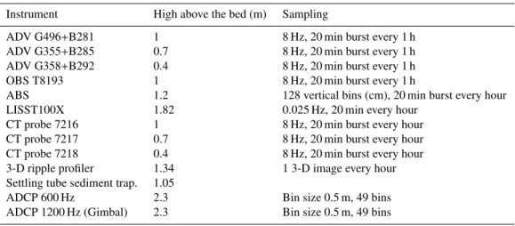
Table 2.Instrumentation in STABLE-III rig deployed in Hilbre Channel.
STABLE-III: Hilbre Channel, 53◦
22.382′
N 3◦
14.147′
W, 14 Feb 2008–11 Mar 2008
Instrument High above the bed (m) Sampling
ADV G496+B281 1 8 Hz, 20 min burst every 1 h
ADV G355+B285 0.7 8 Hz, 20 min burst every 1 h
ADV G358+B292 0.4 8 Hz, 20 min burst every 1 h
OBS T8193 1 8 Hz, 20 min burst every 1 h
ABS 1.2 128 vertical bins (cm), 20 min burst every hour
LISST100X 1.82 0.025 Hz, 20 min every hour
CT probe 7216 1 8 Hz, 20 min burst every hour
CT probe 7217 0.7 8 Hz, 20 min burst every hour
CT probe 7218 0.4 8 Hz, 20 min burst every hour
3-D ripple profiler 1.34 1 3-D image every hour
Settling tube sediment trap. 1.05
ADCP 600 Hz 2.3 Bin size 0.5 m, 49 bins
ADCP 1200 Hz (Gimbal) 2.3 Bin size 0.5 m, 49 bins
flows. Figure 3 shows an example of the despiking algorithm on the data. It can be seen that the method properly removes the spikes. It has to be noted that the data were very clean and only a few spikes were found in the raw time series.
LISST data are treated directly with the manufacturer soft-ware using the calibration information of each instrument. ABS raw data have to be converted to obtain sediment con-centration profile by an inversion algorithm (Betteridge et al., 2008). If the phase of the backscattered signal from a sus-pension of sediments is randomly distributed between 0–2π, the backscattered signal from a multi-frequency ABS can be converted to concentration and mean particle size (Sheng and Hay, 1988; Hay, 1991; Thorne and Campbell, 1992; Thorne and Hanes, 2002). Although using multi-frequency can be used to obtain profiles of particle size and concentration, at this stage in the analysis, advantage has been taken of the sediment trap data located on the frames to obtain estimates for the suspended particle size, and the ABS inversion used these sizes to calculate suspended sediment concentration profiles (Bola˜nos et al., 2009).
Wave parameters can be obtained from ADCP or from combining ADV and pressure data. The PUV method
(Gor-Figure 3. Top: Example of original and despiked ADV time se-ries. Bottom: difference between the series shown in the top panel. Horizontal axis shows time, sampling frequency was of 8 Hz.
pressure spectra to surface elevation spectra:
Cηp=
h cosh(kh) cosh(k(h+z)
i2 Cp
ρ2g2
Cηu=
h sinh(kh) cosh(k(h+z)
i2Cu
σ2
(1)
whereCηpCηu are surface elevation spectra based on pres-sure (Cp) and velocity (Cu) spectra,kis wave number,his the mean water depth relative to the seabed,zis the vertical distance relative to the mean water level,gis gravity andρ
is water density. The frequency limits were set to 0.03 for the lowest frequency and when cosh(kh)=200 for the high frequency.
In order to take into account the background currents the surface wave dispersion relation has been modified following Wolf (1997):
ω=pgktanhkH+kUcosα (2)
ωis frequency
kis the wave number
Uis the background velocity
αangle between currents and waves
The wave direction is estimated by comparing the magni-tude of the cross spectra at each frequency (f):
D=tan−1
(Cpu(f)/Cpv(f)) (3)
CpuCross spectra of pressure anducomponent
CpvCross spectra of pressure andvcomponent
The PUV method is very convenient because it only re-quires a single point velocity and pressure estimations.
The data are being banked at BODC (British Oceano-graphic Data Centre, http://www.bodc.ac.uk) which is the formal British organization for looking after and distributing data concerning the marine environment. The data can be provided from the authors or from S. Gaffney (sgaf@bodc. ac.uk, at BODC). The data policy is consistent with legal frameworks, such as the Environmental Information Regula-tions 2004 and the INSPIRE RegulaRegula-tions 2009. The policy involves a period of 2 years after the collection of the data before it can become available to the public.
5 Environmental conditions during the 2008
deploy-ment period
5.1 Hydrodynamics
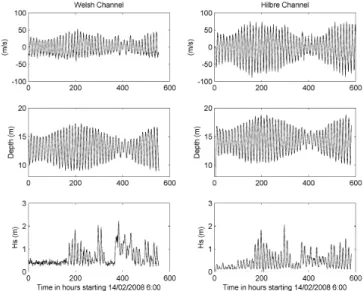
Time series of hydrodynamic parameters at Hilbre channel and Welsh channel during the deployment period are shown in Fig. 4. Current speed is controlled by tides and it fol-lows the spring/neap and flood/ebb cycle. Velocities at Hilbre channel are slightly larger during flood. The Hilbre channel presents larger velocities than the Welsh channel probably
Figure 4.Time series of hydrodynamics at the Welsh Channel (left) and at Hilbre Channel (right). Top panel is current velocity (positive is flood and negative is ebb). Middle panel is water depth. Bottom panel is significant wave height.
due to its position in reference to the central part of the chan-nel. Wave parameters are modulated by tide. The wave event during the second neap period, observed in the Welsh chan-nel, is not present in the Hilbre channel due to a possible dissipation of energy when waves propagate in the estuary mouth. Current direction (not shown) at the Hilbre channel location is aligned with N-S while at the Welsh channel is E-W. The ebbs at the Welsh channel produce a change in cur-rent direction that could be attributed to eddy formation due to curvature of channel, interaction with the fame and with the coastline ledge. Wave direction is predominantly from E and NE at the Welsh channel, however at the Hilbre predomi-nant directions are from north, in agreement with the channel orientation. Mean periods in the area range from 3–6 s and peak period from 4–10 s.
5.2 Sediment in suspension
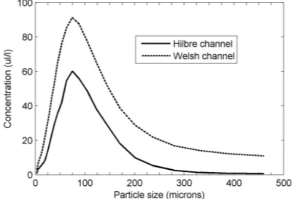
Figure 5. Size distribution of suspended sediment during the first day of deployment.
Figure 6. Time series of integrated parameters from the LISST. Top panel is the concentration. Second panel is the peak size. Third panel is the turbidity from the OBS sensor.
the limit between silt and very fine sand, there is also an im-portant contribution of fine sand (130–250 microns). Both lo-cations show the same pattern in size distribution, but larger concentrations at the Welsh channel possibly due to its more exposed location to wave activity and its closer position to the bed. The large concentration of cohesive particles could support the formation of flocs at some stage of the tidal cycle. Figure 6 shows time series of integrated parameters from the LISST and the OBS at STABLE-III. The suspended sed-iment concentration from the LISST is not clearly related to flood and ebb but there is a signal that correlates with the spring-neap cycle. The peak size of the distribution shows that, in contrary to concentration, large particles are present for both spring and neap tides and this might be controlled by flood and ebb cycle. The turbidity data from the OBS show a very similar pattern to the concentration from the LISST showing a large correlation and a strong neap/spring signal. The mild wave events have a slight effect on sed-iment concentration from the LISST. A rise of concentra-tion and turbidity in the burst 380 that agrees with a wave
Figure 7.Samples of salinity and temperature profiles in the Hilbre Channel during the 14 February 2008. The arrows show the direc-tion at which the profile moves at the start of flood (blue) and ebb (red).
event can be observed. The concentration presents large scat-ter when compared with velocities from ADVs. This shows that the concentration at about 1.5 m above the bed is not a pure representation of bottom processes but it could also involve some flocculation and small particle processes that might need longer time to react to environmental conditions.
5.3 CTD stations
Even though the Dee Estuary is tidal dominated, the strat-ification can be important in turbulence and transport pro-cesses. CTD stations were performed taking advantage of the deployment and recovery manoeuvres of the rigs. Stations were performed every half hour during 24 h if the weather and timing for entering/exiting the channels allowed it. An example of the salinity and temperature profiles in the Hilbre Channel are presented in Fig. 7 where the tidal oscillation of surface stratification can be observed. Close to low tide, a surface low density layer is present, meanwhile near high tide the profiles become more monotonic and with larger salinity due to the entrance of the saline water. The flood currents rise salinity and mix the water column while ebb currents decrease salinity mainly at the surface and produce stratifi-cation.
6 Complementary data
Table 3.Summary of the March 2004 data.
Location Rig/position Instrumentation Other data
Hilbre Channel STABLE-II
53◦ 23.422′ N 03◦ 14.217′ W Ripple profiler LISST ABS CTD Grab sample Bed-frame 53◦ 22.773′ N 03◦ 14.113′ W ADCP Current meter
Welsh Channel Bed-frame
53◦ 22.156′ N 03◦ 19.351′ W ADCP 2 ADV LISST CTD
Table 4.Summary of the February 2005 data.
Location Rig/position Instrumentation Other data
Hilbre Channel STABLE-II
53◦ 22.340′ N 03◦ 14.062′ W 2 ADVs Ripple profiler LISST CT ABS CTD Grab sample Side-scan sonar Bed-frame 53◦ 22.629′ N 03◦ 4.213′ W ADCP
Welsh Channel Bed-frame
53◦ 22.202′ N 03◦ 19.517′ W LISST ADCP Side-scan sonar
STABLE and two bed frames. Similar deployments took place during 2005 and 2006. In 2007, the deployments were extended including Mini-STABLE and the addition of more instruments into the rigs.
Similar to the 2008 campaign, the 2009 was funded by the FORMOST NERC project and it involved the deployment of Mini-Stable and STABLE-III but also included the idea of looking at biological effects, hence it included chlorophyll sampling and two deployments (winter and spring).
7 Conclusions
This work has presented a data set that comprises measure-ments of the relevant bottom processes focused to signifi-cantly advance the understanding of critical aspects of the key sediment transport processes, for example, bedform evo-lution, modes of sediment entrainment and the impact of mixed sediments in combined waves and currents and con-tribute to the improvement of its modelling. The Dee Estu-ary presents particular features, making it an interesting site to study not only because of its local importance but because of the mixed processes taking place there involving tidal hy-drodynamics, wave events, sand and cohesive sediment, bio-logical activity and river influence.
Table 5.Summary of the February 2006 data.
Location Rig/position Instrumentation Other data
Hilbre Channel STABLE-II
53◦ 22.231′ N 03◦ 14.016′ W 2 ADVs Ripple profiler LISST ABS CT Side-scan sonar CTD SMP from water samples Bed-frame 53◦ 22.944′ N 03◦ 14.216′ W ADCP
Welsh Channel Bed-frame
53◦ 22.196′ N 03◦ 19.471′ W ADCP
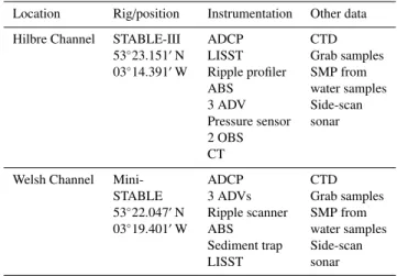
Table 6.Summary of the March 2007 data.
Location Rig/position Instrumentation Other data
Hilbre Channel STABLE-III
53◦ 23.151′ N 03◦ 14.391′ W ADCP LISST Ripple profiler ABS 3 ADV Pressure sensor 2 OBS CT CTD Grab samples SMP from water samples Side-scan sonar
Welsh Channel
Mini-STABLE 53◦ 22.047′ N 03◦ 19.401′ W ADCP 3 ADVs Ripple scanner ABS Sediment trap LISST CTD Grab samples SMP from water samples Side-scan sonar
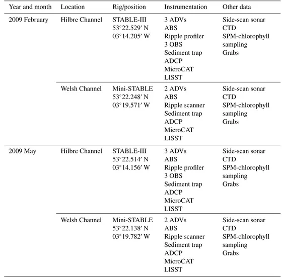
Table 7.Summary of the 2009 data.
Year and month Location Rig/position Instrumentation Other data
2009 February Hilbre Channel STABLE-III 53◦
22.529′
N 03◦
14.205′
W
3 ADVs ABS
Ripple profiler 3 OBS Sediment trap ADCP MicroCAT LISST
Side-scan sonar CTD
SPM-chlorophyll sampling Grabs
Welsh Channel Mini-STABLE 53◦
22.248′
N 03◦
19.571′
W
2 ADVs ABS
Ripple scanner Sediment trap ADCP MicroCAT LISST
Side-scan sonar CTD
SPM-chlorophyll sampling Grabs
2009 May Hilbre Channel STABLE-III 53◦
22.514′
N 03◦
14.156′
W
3 ADVs ABS
Ripple profiler 3 OBS Sediment trap ADCP MicroCAT LISST
Side-scan sonar CTD
SPM-chlorophyll sampling Grabs
Welsh Channel Mini-STABLE 53◦
22.138′
N 03◦
19.782′
W
2 ADVs ABS
Ripple scanner Sediment trap ADCP MicroCAT LISST
Side-scan sonar CTD
SPM-chlorophyll sampling Grabs
This data set is ideal for testing hydrodynamic, turbulence and sediment transport models and critically assess the im-provement in the transport predictions that arise from the clusion of a range of detailed transport processes. These in-clude improved bed roughness prediction, representation of the “wave-related” transport component, effects of a mixed sediment bed and the extent to which our predictive capabil-ities related to sand transport remain valid in a mixed sedi-ment environsedi-ment.
Acknowledgements. The authors would like to thank the Prince Madog crew for their support during the deployment and recovery of the moorings. Support from the engineering group at POL is greatly acknowledged. This work was partially funded by NERC FORMOST project and NERC Oceans 2025 programme. Authors thank the support from S. Gaffney at BODC.
Edited by: G. M. R. Manzella
References
Baumert, H., Chapalain, G., Smaoui, H., McManus, J. P., Yagi, H., Regener, M., Sundermann, J., and Szilagy, B.: Modelling and numerical simulation of turbulence, waves and suspended sed-iments for pre-operational use in coastal seas, Coast. Eng., 41, 63–93, 2000.
Betteridge, K. F. E., Thorne, P. D., and Cook, R. D.: Calibrating multi-frequency acoustic backscatter system for studying near-bed suspended sediment transport processes, Cont. Shelf Res., 28, 227–235, 2008.
Bola˜nos, R., Riethmuller, R., Gayer, R., and Amos, C. L.: Sedi-ment transport in a tidal lagoon subject to varying winds evalu-ated with a coupled current-wave model, J. Coast. Res., 21, e11– e26, 2005.
Brown, J. M. and Wolf, J.: Coupled wave and surge modelling for the eastern Irish Sea and implications for model wind-stress, Cont. Shelf Res., 29, 1329–1342, 2009.
Crawford, A. M. and Hay, A. E.: Determining suspended sand size and concentration from multifrequency acoustic backscatter, J. Acoust. Soc. Am., 94, 3312–3343, 1993.
GOOS: The integrated strategic design plan for the coastal ocean observations module of the global ocean observing system, 190, 2003.
Gordon, L. and Lohrman, A.: Near-shore Doppler current meter wave spectra, Ocean wave measurement and analysis, ASCE Waves 2001 Conference, 33–43, 2001.
Goring, D. G. and Nikora, V. I.: Despiking acoustic Doppler ve-locimeter data, J. Hydrau. Eng., 128(1), 117–126, 2002. Hay, A. E.: Sound scattering from a particle-laden turbulent jet, J.
Acoust. Soc. Am., 90, 2055–2074, 1991.
Hutchinson, S. M.: Distribution of137Cs in saltmarsh sediments in the Dee Estuary, NW England, Mar. Pollut. Bull., 28, 4, 262– 265, 1994.
Hutchinson, S. M. and Prandle, D.: Siltation in the saltmarsh of the Dee Estuary derived from137Cs analysis of shallow cores, Estuar. Coast. Shelf S., 38, 5, 471–478, 1994.
Longuet-Higgins, M. S., Cartwright, D. E., and Smith, N. D.: Ob-servations of the directional spectrum of the sea waves using the motions of a floating buoy, Ocean Wave Spectra, Prentice-Hall, 111–136, 1963.
Mastenbroek, C., Burgers, G., and Janssen, P. A. E. M.: The dynam-ical coupling of a wave model and a storm surge model through the atmospheric boundary layer, J. Phys. Oceanogr., 23, 1857– 1866, 1993.
Moore, R. D., Wolf, J., Souza, A. J., and Flint, S. S.: Morpholog-ical evolution of the Dee Estuary, Eastern irish sea, UK: a tidal asymmetry approach, Geomorphology, 103, 588–596, 2009. Mori, N., Suzuki, T., and Kakuno, S.: Noise of Acoustic Doppler
Velocimeter data in bubbly flows, J. Eng. Mechanics, 133, 122– 125, 2007.
Pinardi, N. and Woods, J.: Ocean Forecasting, Conceptual basis and applications, Springer, 2002.
Sheng, J. and Hay, A. E.: An examination of the spherical scatterer approximation in aqueous suspensions of sand, J. Acoust. Soc. Am., 83, 598–610, 1988.
Simpson, J. H., Fisher, N. R., and Wiles, P.: Reynolds stress and TKE production in an estuary with a tidal bore, Estuarine, Coast. Shelf Sci., 60, 619–627, 2004.
Souza, A. J., Dickey, T. D., and Chang, G. C.: Modeling water column structure and suspended particulate matter on the Mid-dle Atlantic continental shelf during the passages of Hurricanes Edouard and Hortense, J. Mar. Res., 59, 1021–1045, 2001. Styles, R.: Laboratory evaluation of the LISST in a stratified fluid,
Mar. Geol., 227, 151–162, 2006.
Thorne, P. D. and Campbell, S. C.: Backscattering by a suspension of spheres, J.Acost. Soc. Am., 92, 978–986, 1992.
Thorne, P. D. and Hanes, D. M.: A review of acoustic measurements of small-scale sediment processes, Cont. Shelf Res., 22, 603– 632, 2002.
Wahl, T. L.: Discussion of “Despiking acoustic doppler velocimeter data”, J. Hydr. Eng., 129(6), 484–487, 2003.
Williams, J. J., Bell, P. S., Coates, L. E., Metje, N., and Selwyn, R.: Interactions between a benthic tripod and waves on a sandy bed, Cont. Shelf Res., 23, 355–375, 2003.
Williams, J. J., Bell, P. S., Thorne, P. D., Metje, N., and Coates, L. E.: Measurement and prediction of wave-generated suborbital ripples, J. Geophys. Res., 109, C02004, doi:10.1029/2003JC001882, 2004.
Williams, J. J., Bell, P. S., and Thorne, P. D.: Unifying large and small wave-generated ripples, J. Geophys. Res., 110, C02008, doi:10.1029/2004JC002513, 2005.
Wolf, J.: The analysis of bottom pressure and current data for waves, Proceedings of the 7th International Conference on Elec-tronic Engineering in Oceanography, Southampton, Conference Publication 439, 1997.