SCALING OF SEMIVARIOGRAMS AND THE KRIGING ESTIMATION OF FIELD-MEASURED PROPERTIES

SCALING OF SEMIVARIOGRAMS AND THE KRIGING

ESTIMATION OF FIELD-MEASURED PROPERTIES

S. R. VIEIRA(2), P. M. TILLOTSON(3), J. W. BIGGAR(4 ) & D. R. NIELSEN(4)

SUMMARY

Two methods were evaluated for scaling a set of semivariograms into a unified function for kriging estimation of field-measured properties. Scaling is performed using sample variances and sills of individual semivariograms as scale factors. Theoretical developments show that kriging weights are independent of the scaling factor which appears simply as a constant multiplying both sides of the kriging equations. The scaling techniques were applied to four sets of semivariograms representing spatial scales of 30 x 30 m to 600 x 900 km. Experimental semivariograms in each set successfully coalesced into a single curve by variances and sills of individual semivariograms. To evaluate the scaling techniques, kriged estimates derived from scaled semivariogram models were compared with those derived from unscaled models. Differences in kriged estimates of the order of 5% were found for the cases in which the scaling technique was not successful in coalescing the individual semivariograms, which also means that the spatial variability of these properties is different. The proposed scaling techniques enhance interpretation of semivariograms when a variety of measurements are made at the same location. They also reduce computational times for kriging estimations because kriging weights only need to be calculated for one variable. Weights remain unchanged for all other variables in the data set whose semivariograms are scaled.

Index terms: semivariogram, scaling, kriging, spatial variability.

RESUMO: ESCALONAMENTO DE SEMIVARIOGRAMAS E A ESTIMATIVA DE

PROPRIEDADES MEDIDAS A CAMPO PELO MÉTODO DE KRIGAGEM.

Foram avaliados dois métodos de escalonamento de semivariogramas, para obter uma única função de ajuste e estimar propriedades medidas, no campo, por meio da krigagem. No escalonamento, utilizaram-se, como fatores de escala, a variância das amostras e os patamares dos semivariogramas. Os desenvolvimentos teóricos mostram que os ponderadores da krigagem são independentes dos fatores de escala, os quais aparecem, simplesmente, como uma constante que multiplica os dois lados das equações de krigagem. As técnicas de escalonamento foram aplicadas a quatro conjuntos de semivariogramas, representando escalas de 30 x 30 m até 600

(1) _{Received for publication in September 1996 and aproved in June 1997.}

(2) _{Researcher of Instituto Agronômico de Campinas, Caixa Postal 28, CEP 13001-970, Campinas (SP).} (3) _{Assistent Professor, Department of Agronomy, University of Georgia, Griffin, GA 30223-1797.} (4) _{Professor, Department of Land, Air and Water Resources, University of California, Davis, CA 95616.}

x 900 km. Semivariogramas experimentais de cada conjunto foram coalescidos, com sucesso, em uma curva única, usando, como fatores de escala, tanto as variâncias como os patamares dos semivariogramas. Para avaliar as técnicas de escalonamento, estimativas feitas com semivariogramas escalonados foram comparadas com as efetuadas com modelos não escalonados. Nos casos em que o escalonamento não coalesceu os semivariogramas individuais, foram encontradas diferenças da ordem de 5% entre valores estimados com krigagem sem escalonamento e com escalonamento, o que também significa que essas propriedades variam de maneira diferente no espaço. As técnicas de escalonamento propostas ajudaram a interpretação de semivariogramas, quando várias medições foram feitas para os mesmos locais. Elas também reduziram o tempo de processamento computacional para as estimativas de krigagem, porque os ponderadores da krigagem precisam ser calculados para apenas uma das variáveis. Os ponderadores foram os mesmos para todas as outras variáveis no conjunto de dados cujos semivariogramas foram escalonados.

Termos de indexação: Semivariogramas, escalonamento, krigagem, variabilidade espacial.

INTRODUCTION

Progress in computing devices and laboratory analysis technology have made it possible to collect large numbers of samples to characterize spatial variability of field-measured soil and climatological properties. As a result, time series analysis and geoestatistical methods have become available for in depth descriptions of spatial variability (Campbell, 1978; Hajrasuliha et al., 1980; Burgess & Webster, 1980; Vieira et al., 1981; Nielsen et al., 1983).

Common characterization of variability has been accomplished with autocorrelograms, semivariograms, spectral analysis and kriging estimation (Webster and Cuanalo, 1975; Vieira et al., 1981; Vieira et al., 1983; Vauclin et al., 1983; Libardi et al., 1986; Kachanoski & Jong, 1988). Autocorrelograms disclose the length of spatial dependence but require strong stationarity assumptions that are not commonly found, nor easily verified in the field. Subsequent analysis through the Fourier transform of the autocorrelogram makes it possible to study partitioning of sample variance into important frequency components through spectral analysis (Shumway, 1988). Semivariograms, on the other hand, require weaker stationary assumptions, but provide straightforward spatial interpretations through kriging estimation. The existence of spatial dependence through the semivariogram provides the necessary requirement for application of the kriging method to interpolate measurements in the field without bias and with minimum variance. Kriged contour or three dimensional maps are popular representations of spatial variability results (Hajrasuliha et al., 1980; Burgess and Webster, 1980; MacBratney et al., 1982; Vauclin et al., 1983) and provide quantitative assessments of variability.

While our ability to assess spatial variability on a single soil or climatological property has improved significantly, integration of observations of more than one variable has lagged considerably. Vachaud et al. (1985) showed that time stability of the spatial variability may exist for water content measured on the same locations at different times. Kachanoski et al. (1988) applied coherence analysis techniques to water content measured at the same locations with

TDR method, making use of the autocorrelation function, and, therefore, assuming second order stationarity. Scaling semivariograms of several variables measured over the same region provides a simple but powerful integration method (Vieira et al., 1988, Vieira et al., 1991). This paper further develops theoretical aspects of the proposed scaling technique of Vieira et al. (1988) and Vieira et al. (1991) and provides examples of its application.

MATERIAL AND METHODS

Theory

The experimental semivariogram, γ(h), of n spatial observations z(xi), i = 1,...n, can be calculated using

γ

(h) =

1

2N(h)

[z(x ) - z(x + h)]

i i

2

∑

where N(h) is the number of observations separated by a distance h. Experimental semivariograms can be fit to a variety of models that have well known parameters: nugget C₀, sill (C₀ + C₁), and range of spatial dependence a(5)_{. Equation [1] is obtained from}

a derivation starting at the intrinsic assumption, under which there is no requirement for existence of a finite variance of the observations, Var(z). Only stationary of the mean and second order stationarity of the differences [(z(x_i)-z (x_i + h)] are required for its derivation (Journel & Huijbregts, 1978; p.11).

Vieira et al. (1991) proposed a scaling technique for the semivariogram expressed by

sc

(h) =

(h)

Var(z)

γ

γ

(5) _{The two semivariogram models used in this study are:} - exponential - denoted in the figures as Exp (C₀; C₁; a)

γ(h) = C₀+C₁ [1 - exp(-3h/a)]

- spherical - denoted in the figures as Sph (C₀; C₁; a)

Thus, the kriging variance σk2 for each individual

variable, l , is

[

]

k l 0 l

i=1 n

i sc

i 0

(x ) = +

(x ,x )

σ

µ α

λ γ

∑

The scaling technique does not change the weights λi since the scaling factor is simply a multiplied

constant on both sides of the first equation of the kriging system [6].

The system of equations [6] is valid for both unique and sliding neighborhood options during kriging estimation. The unique neighborhood uses the entire data set for each estimation throughout the field. That means that the kriging system [6] is solved by inverting the coefficient matrix of γsc_(x

i, xj) only once,

then multiplying the inverted matrix by the right hand side, γsc_(x

i,x0), for each location, since it is only a

function of the estimated location x0. This technique

may not be feasible for large data sets owing to the difficulty or cost in inverting large matrices. The sliding neighborhood technique is useful in this situation since it uses a reduced neighborhood for each kriging estimation. This means that the kriging system [6] must be solved for each estimation.

The scaling technique simplifies the kriging estimation process for either of the neighborhood options when several variables are measured at the same location. For the unique neighborhood, the procedure is to invert the coefficient matrix (which is the same for all variables), store it, calculate the right hand side for the first variable, store it for calculation of the kriging variance [7], and obtain the weights λi

through matrix multiplication. The weights can then be used for kriging estimation of all variables in the data set. Similarly, for the sliding neighborhood option, the right hand side γsc_(x

i,x0) must be calculated and

the kriging system [6] solved only for the first variable to be estimated.

The proposed scaling concept will be used on data sets from four different geographic locations. Within each data set, a single scaled semivariogram for all variables for a particular location will be sought, and kriged estimates and kriging variances for each variable using its individual semivariogram (Equation. [1]) with those using the scale semivariogram will be compared.

When data of several variables coalesce into a unified semivariogram structure, it is possible to take advantage of variables having the same spatial structure and, hence, reduce the number of semivariograms needed to analyze and draw interpretations regarding their spatial values. However, if coalescence of the individual semivariograms is not adequate, with some variables indeed having different scaled semivariograms than that of the overall scaled semivariogram, the kriged estimation variances will differ. On the other hand, kriged estimates are much less sensitive to the semivariogram model, and therefore, it is expected their values from both scaled and unscaled systems to be nearly the same.

where γsc_{(h) is the scaled semivariogram,} γ_{(h) the}

original semivariogram, and Var(z) the sample variance of the observations. In theory, this equation requires the existence of a finite variance which can be guaranteed if second order stationarity exists. However, this condition does not always exist and is not easily verified in practice.

To overcome the lack of second order stationarity, yet using the covariance function during kriging estimation, Journel & Huijbrets, 1978; p.306) recommended a “pseudo-covariance” C(h) such that:

C(h) = A - (h)

γ

where A is any positive constant greater than the largest γ(h) to guarantee a positive covariance. The value of A is canceled in the derivation of the kriging system because of the unbiased condition. Here, a similar approach is used, and equation [2] is generalized to be

sc

i

(h) =

(h) /

l = 1, 2,..., m

γ

γ

α

were m indicates the number of measured variables. The scale factor α is a constant that can take the value of the calculated variance, the sill when it exists, or the highest value of the semivariogram γ(h).

Two facts are very important about the above theoretical concepts: i) The semivariogram γ(h) is assumed to be isotropic, i.e., either there is no significant anisotropy or there is a transformation before scaling is applied; ii) α can take the value of the calculated variance Var(z) no matter whether it represents the true variance or not, since the scaling factor is simply a number chosen to make the semivariograms coalesce into a single curve. The difference between equations [2] and [4] is conceptual inasmuch as equation [2] is linked to the Var(z) value which requires second order stationarity, while the scaling factor as in equation [4] can, in principle, take any value ranging from the sample variance to the maximum value of γ(h), as long as the scaling factors remain identified with corresponding variables for unscaling purposes.

The kriging estimator z*_(x

0) at location x0 remains

the same as without scaling:

* 0

i=1 n

i i

z (x ) =

∑ λ

z(x )

where λi is the kriging weight associated with

observation i at location xi. When submitted to

unbiasedness and minimum variance conditions, the kriging system, in terms of the scaled semivariogram, becomes

j=1 n

j sc

i j

sc i 0

j=1 n

j

(x , x ) + = (x , x ) i = 1, 2,..., n

= 1

∑

∑

λ γ µ γ

λ

[6]

Data sets

Rainfall - Banzatto & Benincasa (1986) compiled rainfall data on maximum probable daily rainfall for return periods of 5, 10, 25, 50 and 100 years. Data were collected for at least 20 years from 206 raingauge stations distributed over an area which spanned 600 x 900 km. Longitudes and latitudes were used to transform the UTM coordinate system to a (X, Y) coordinate system in kilometers. The procedure for calculation of maximum probable daily rainfall involved application of the Gumbel probability density function constructed for each location with parameters based upon a long series of data. It is obvious that maximum rainfall values increase with the return period, but the spatial distribution of each return period, could only be autocorrelated, if the rainfall generating process for the state remained approximately constant over the 20 year period.

Soil fertility - A study was conducted in Campinas, State of São Paulo, Brazil to characterize spatial variations of the fertility status of an Oxisol on a scale commensurate with randomized block experiments. The 30 x 30 m field was sampled on a 5 m square grid spacing yielding a total of 49 sample locations. Soil samples were collected from the 0-25 and 25-50 cm layers and analyzed for routine chemical and physical constituents suitable for fertilizer recommendation. The cation exchange capacity (CEC), sum of bases, delta pH and base saturation were calculated from the chemical analyses.

Soil organic carbon and nitrogen - Waynick & Sharp (1919) conducted variability studies on a sandy soil in Oakley, California and on a silty clay loam soil in Davis, California, USA. One hundred samples from the topsoil of each field were collected on a 9.1 x 9.1 m grid with additional samples taken at 3.0 and 4.6 m in some locations. Soil samples were analyzed for organic carbon and total nitrogen.

Soil moisture content - One hundred and sixty four TDR (time domain reflectometry) rods were installed in a Rideau clay loam soil in the Central Experimental Farm of Agriculture Canada, Ottawa, for measuring volumetric water content of the surface 0.2 m of soil. The triangular field, 120 m in the x-direction (base) and 220 m in the y-direction (height), was divided into a 10 x 10 m grid. All water content measurements over the field were collected within a two hour time period.

RESULTS AND DISCUSSION

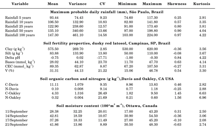
Main statistical moments of all variables from the four geographic locations are shown in table 1. Semivariogram for individual return periods of maximum probable daily rainfall are show in figure 1a as log(γ(h)). Inasmuch as an almost exact repetition of pattern exists among them, some scale factor should make them coalesce into a single curve. Besides being similar, they increase exactly in order from 5 to 100

Table 1. Statistical moments for the data

Variable Mean Variance CV Minimum Maximum Skewness Kurtosis Maximum probable daily rainfall (mm), São Paulo, Brazil

Rainfall 5 years 93.44 74.43 9.23 74.60 117.30 0.25 2.91

Rainfall 10 years 106.50 132.90 10.83 82.80 141.80 0.57 3.35

Rainfall 25 years 122.90 238.60 12.57 91.00 173.40 0.80 3.81

Rainfall 50 years 135.10 340.60 13.66 97.00 198.80 0.90 4.04

Rainfall 100 years 147.30 461.10 14.58 103.00 224.00 0.97 4.22

Soil fertility properties, dusky red latosol, Campinas, SP, Brazil

Clay (g kg-1) 575.50 269.70 2.85 530.00 620.00 -0.36 3.56

Silt (g kg-1) 83.88 133.90 13.80 50.00 110.00 -0.08 3.67

Delta pH -0.75 0.02 -17.71 -1.00 -0.30 0.84 4.22

Bases (mmol_c kg-1) 28.02 44.10 23.70 11.70 47.70 0.63 4.14

CEC (mmol_c kg-1) 89.35 62.87 8.87 67.20 107.50 -0.27 3.31

V (%) 31.31 44.13 21.22 15.06 46.78 0.54 3.30

Soil organic carbon and nitrogen (g kg-1

),Davis and Oakley, CA USA

C-Davis 11.11 1.079 9.35 8.96 13.83 0.46 2.82

N-Davis 0.10 0.008 9.14 0.77 1.18 -0.25 2.88

C-Oakley 4.33 1.316 26.49 1.82 9.50 1.45 6.63

N-Oakley 0.32 0.004 21.69 0.21 0.60 1.56 6.96

Soil moisture content (100*m3

m-3

), Ottawa, Canada

11/September 28.38 32.25 20.01 17.00 43.20 0.31 2.50

14/September 42.81 18.59 10.07 30.90 54.50 -0.36 3.06

17/September 37.26 18.33 11.49 27.00 45.20 -0.10 2.08

years of return period, indicating that maximum rainfall increases proportionally to the return period everywhere in the entire state. Scaling factors used in this case were the corresponding variances given in Table 1. The individual semivariogram for ten years return period is shown in figure 1b with an exponential model. The overall scaled semivariogram fitted with the exponential model is shown in figure 1c. The coalescence of the five semivariograms into a single curve is remarkably good, and supports the choice of the scale factors. There are some points between 50 and 100 m which indicate periodicity at short distances within the data set. This behavior was verified and represents increases in rainfall within short distances in some particular mountainous regions of the state. However, results of the jack-knifing procedure in kriging estimation favored an exponential semivariogram model over that of a hole effect model, indicating that periodicity is apparently not important for nonmountainous parts of the state. If desired, the mountainous zone could be analyzed separately.

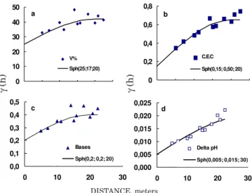
Individual semivariograms for the soil fertility study in Campinas, SP, Brazil, are shown in figure 2 in separated graphs because of their wide range of values. The highest variance value (and sill) is for base saturation percentage (V %) shown in figure 2a, which being a composite variable tends to accumulate variability from its different components. Although they were fitted to the same type of model equation (spherical), there is not an apparent similarity among the semivariograms. Except for delta pH, each has a relatively large nugget, reaches the sill at about the same range and fits reasonably well to the spherical models shown by solid lines (Figure 2).

Scaling of semivariograms for soil fertility data using sills of corresponding individual semivariograms is shown in figure 3a and the results using the corresponding variances of each variable is shown in figure 3b. Scaling with variances of each individual property appears to be slightly better because of the reduced scatter around the unique spherical model, and because the resulting sill equals one, as compared to 1.1 for the other approach. Both approaches produced scaled semivariograms having exactly the same range of spatial dependence as individual semivariograms. Comparing scaling of these semivariograms with those for the maximum probable daily rainfall in the State of São Paulo, the coalescence of soil properties is not as good, probably because the similarity in soil properties is not as strong as that of rainfall for different return periods. In this case, it also means that the soil fertility properties have different spatial variabilities. Vieira et al. (1988) found scaled semivariograms for soil moisture and saturated hydraulic conductivity at 0.2 m depth to be very different and at 0.5 m depth to be very similar, because the soil structure at 0.2 m depth is very strong and controls water flow through macropores, but water is within peds. At 0.5 m, the massive structure both holds the water and controls the flow, and for this reason, these properties have similar semivariograms. a

1 10 100 1000

Log[

γ

(h)]

5 years 10 years 25 years 50 years 100 years

c

0,0 0,2 0,4 0,6 0,8 1,0 1,2

0 100 200 300 400

γ

sc (h)

5 years 10 years 25 years 50 years 100 years

Exp(0,35; 0,65; 100) b

0 50 100 150 200

γ

(h)

10 years Exp(50;80;100)

Figure 1. Semivariograms for maximum daily rainfall in São Paulo. a) On a log scale; b) For maximum daily rainfall at 10 years return period; c) Scaled semivariograms with a single model.

Figure 2. Individual semivariograms for chemical properties at 0-0,25 m in Oxisol, Campinas SP, Brazil. a) Base saturation; b) Cation exchange capacity; c) Sum of bases; d) Delta pH.

DISTANCE, km DISTANCE, meters

b

0 0,2 0,4 0,6 0,8

C.E.C Sph(0,15; 0,50; 20)

d

0,000 0,005 0,010 0,015 0,020 0,025

0 10 20 30

Delta pH Sph(0,005; 0,015; 30)

c

0,0 0,1 0,2 0,3 0,4 0,5

0 10 20 30

Bases Sph(0,2; 0,2; 20)

a

0 10 20 30 40 50

V% Sph(25;17;20)

γ

(h)

γ

b

0,0 0,2 0,4 0,6 0,8 1,0 1,2 1,4

0 10 20 30

De lta pH Ba se s C.E.C. V % S ph(0,4; 0,6; 20)

Figure 3. Scaled semivariograms for the chemical properties at 0-0,25 m in Oxisol, Campinas SP, Brazil. a) Scaling factor equals the sill of individual semivariograms. b) Scaling factor equals the calculated variance of each property.

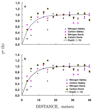
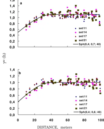
Semivariograms for organic carbon and nitrogen are shown in figure 4. All are fitted by a spherical model. For the sandy soil from Oakley, the sill appears to be more obvious. The scaled semivariograms corresponding to figure 4 are shown in figure 5a and b for scaling with sills of individual semivariograms and the variances, respectively. The two kinds of scaling factors produced similar results as far as their efficiency in coalescing individual semivariograms and both of them did not appear to be very appropriated. Soil moisture contents in Ottawa showed similar sets of semivariograms (Figure 6). Their scaled semivariograms coalesced without much scatter (Figure 7). The two methods of scaling the semivariograms did not seem to have any advantage over the other. The only difference between scaled semivariograms in figure 7a and b is the value of their sills. Scaling using individual sills produced a semivariogram with a sill of 1.1 as compared with 1.0 for those scaled with individual variances. The reason for this may be that the individual sills are, in fact, somewhat lower than the individual variances. Because of this similarity, not much difference should be expected in their ability to estimate individual values. However, it should be emphasized that the scaling factor can be the value of the calculated sample variance, but, not necessarily, the theoretical variance associated with corresponding probability distributions. The primary reason for this is to avoid the necessity of satisfying second order stationariness to guarantee the existence of a finite variance.

Figure 5. Scaled semivariograms for the carbon and nitrogen at Oakley and Davis. a) Scaling factor equals the sill of individual semivariograms. b) Scaling factor equals the calculated variance of each property.

DISTANCE, meters

Figure 4. Individual semivariograms. a) Nitrogen Oakley. b) Carbon Oakley. c) Nitrogen Davis. d) Carbon Davis.

DISTANCE, meters

a

0 , 0 0 0 0 , 0 0 1 0 , 0 0 1 0 , 0 0 2 0 , 0 0 2 0 , 0 0 3 0 , 0 0 3 0 , 0 0 4

N itro g e n O a k le y S p h (0 ; 2 ,7 E -3 ; 2 0 )

b

0 0,2 0,4 0,6 0,8

C arbon Oakley Sph(0,3; 0,35; 18)

c

0 ,0 0 0 0 ,0 0 1 0 ,0 0 2 0 ,0 0 3 0 ,0 0 4 0 ,0 0 5 0 ,0 0 6

N itro g e n D a v is S p h (0 ; 4,6 E -3 ; 1 0)

d

0,0 0,1 0,2 0,3 0,4 0,5 0,6 0,7

0 10 20 30 40

C arbon Davis S ph(0; 0,55; 12)

a

0,0 0,2 0,4 0,6 0,8 1,0 1,2

Delta pH Base s C.E.C. V% Sph(0,5; 0,6; 25)

γ

sc (h)

DISTANCE, meters

γ

(h)

b

0,0 0,2 0,4 0,6 0,8 1,0 1,2 1,4

0 10 20 30 40

Nitrogen Oakley Carbon Oakley Nitrogen Davis Carbon Davis Exp(0; 1; 15)

a

0,0 0,2 0,4 0,6 0,8 1,0 1,2 1,4

Nitrogen Oakley Carbon Oakley Nitrogen Davis Carbon Davis Exp(0; 1; 15)

γ

b

0 2 4 6 8 10 12 14

set/14 Sph(3; 8; 44)

a

0,0 0,2 0,4 0,6 0,8 1,0 1,2 1,4 1,6

set/11 set/14 set/17 set/21 Sph(0,4; 0,7; 40)

DISTANCE, meters

Figure 7. Scaled semivariograms for soil moisture content at 0.2 m depth for the Rideau clay loam Ottawa, Canada. a) Scaling factor equals the sill of individual semivariograms. b) Scaling factor equals the calculated variance of each property.

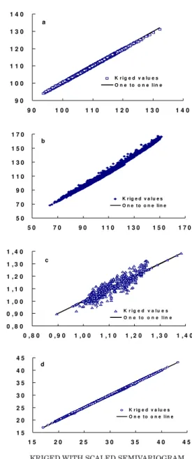
It was shown in previous figures that scaling of semivariograms is both possible and useful in simplifying interpretations of spatial structure in several field-measured variables. Next, applications of scaled semivariograms to kriging estimations will be discussed. The comparisons of kriging estimations using scaled and unscaled semivariograms are presented in figure 8. The proximity of paired values of 5-year return period daily rainfall to the one-to-one line (Figure 8a) indicates how well the scaled semivariogram represents variability in the original data values. As it can be seen, the values estimated with the scaled semivariogram are, in fact, nearly identical to those estimated with individual semivariograms. These results suggest that there is no significant difference in weights obtained from solution of the kriging system for scaled and unscaled semivariograms. Although there is clearly a relationship for cation exchange capacity, CEC, approaching the one-to-one line, the kriging estimation using the overall scaled semivariogram slightly underestimated low values and overestimated large values (Figure 8b). It is possible that this small discrepancy may be due to differences between the unscaled semivariogram for CEC and the overall scaled semivariogram of the entire data set. Kriged values of organic carbon and nitrogen calculated from unscaled semivariograms did not compare favorably with those calculated from the overall scaled

Figure 6. Individual semivariograms for soil moisture content at 0.2 m depth for the Rideau clay loam, Ottawa, Canada. In (a) Data for September/11; (b) Data for September/14; (c) Data for September/17; (d) Data for September/21.

c

0 2 4 6 8 10 12 14

set/17 Sph(5; 6; 30)

d

0 2 4 6 8 10 12

0 20 40 60 80 100

set/21 Sph(3,5; 5,5; 40)

DISTANCE, meters

a

0 2 4 6 8 10 12 14 16

set/11 Sph(6; 7; 32)

b

0,0 0,2 0,4 0,6 0,8 1,0 1,2 1,4

0 20 40 60 80 10 0

set/11 set/14 set/17 set/21 S ph(0,4; 0,6; 40)

γ

sc (h)

γ

2. The choice of scaling factor is not restricted to the statistically defined unbiased variance, but can include sills of original semivariograms. Scaling individual semivariograms with the variance values was more efficient in coalescing of the semivariograms into one single model and had the added advantage of yielding a scaled sill of 1.0.

3. Kriging weights derived from scaled and unscaled kriging systems are not significantly different, as shown by good correspondence between kriging estimates from scaled and unscaled semivariogram values.

REFERENCES

BANZAT T O, D.A. & BENINCASA, M. Estimativa de precipitações máximas prováveis com duração de um dia, para o Estado de São Paulo. Jaboticabal, UNESP, 1986. 36p. (Boletim Técnico 07)

BURGESS, T.M. & WEBSTER, R. Optimal interpolation and isarithmic mapping of soil properties. I. The semivariogram and punctual kriging. J. Soil Sci., Oxford, 31:315-331, 1980.

CAMPBELL, J.B. Spatial variation of sand content and pH within single contiguous delineation of two soil mapping units. Soil Sci. Soc. Am. J., Madison, 42:460-464, 1978.

HAJRASULIHA, S.; BANIABBASSI, J.; METTHEY & NIELSEN, D.R. Spatial variability of soil sampling for salinity studies in southwest Iran. Irrig. Sci., Berlin, 1:197-208, 1980.

JOURNEL, A.G. & HUIJBREGTS, C.H.J. Mining geoestatistics. London, Academic Press, 1978. 600p.

KACHANOSKI, R.G. & JONG, E. Scale dependence and the temporal persistence of spatial patterns of soil water storage. Water Res. Res., Washington, 24:85-91, 1988.

LIBARDI, P.L.; PREVEDELLO, C.L.; PAULETTO, E.A. & MORAES, S.O. Variabilidade espacial da umidade, textura e densidade de partículas ao longo de uma transecção. R. bras. Ci. Solo, Campinas, 10:85-90, 1986.

MacBRATNEY, A.B.; WEBSTER, R.; McLAREN, R.G. & SPIERS, R.E.B. Regional variation of extractable copper and cobalt in the topsoil of southwest Scotland. Agronomie, Paris, 2:969-982, 1982.

NIELSEN, D.R.; TILLOTSON, P.M. & VIEIRA, S.R. Analyzing field-measured soil-water properties. Agric. Water Manag., Amsterdam, 6:93-109, 1983.

SHUMWAY, R.H. Applied statistical time series analysis. Ennglewood, Prentice Hall, 1988. 379p.

VACHAUD, G.; PASSERAT DE SILANE, A.; BALABANIS, P. & VAUCLIN, M.. Temporal stability of spatially measured soil water probability density function. Soil. Sci. Soc. Am. J., Madison, 49:822-827, 1985.

semivariogram for the California soils. As shown in figure 8d, a very good one-to-one relationship for kriged values of soil moisture content measured on September 11, reflecting a good correspondence between scaled and unscaled semivariograms.

CONCLUSIONS

1. Reasonable coalescence of experimental semivariograms into a single function can be accomplished with scaling techniques described when properties show similar spatial structure.

Figure 8. One to one plots. a) Maximum daily rainfall at 10 years return period, São Paulo; b) Cation Exchange Capacity for Dusky Red Latossol, Campinas SP; c) Organic carbon content for Davis soil, Davis CA USA; c) Soil moisture content for 0.2 m depth, Rideau clay loam Ottawa, Canada.

KRIGED WITH SCALED SEMIVARIOGRAM

KRIGED WITH

INDIVIDU

AL

SEMIV

ARIOGRAM

d

1 5 2 0 2 5 3 0 3 5 4 0 4 5

1 5 2 0 2 5 3 0 3 5 4 0 4 5

K r ig e d v a lu e s O n e t o o n e lin e

c

0 , 8 0 0 , 9 0 1 , 0 0 1 , 1 0 1 , 2 0 1 , 3 0 1 , 4 0

0 , 8 0 0 , 9 0 1 , 0 0 1 , 1 0 1 , 2 0 1 , 3 0 1 , 4 0

K r i g e d v a l u e s O n e t o o n e l i n e

b

5 0 7 0 9 0 1 1 0 1 3 0 1 5 0 1 7 0

5 0 7 0 9 0 1 1 0 1 3 0 1 5 0 1 7 0

K r ig e d v a lu e s O n e t o o n e lin e

a

9 0 1 0 0 1 1 0 1 2 0 1 3 0 1 4 0

9 0 1 0 0 1 1 0 1 2 0 1 3 0 1 4 0

VAUCLIN, M.; VIEIRA, S.R.; VACHAUD, G. & NIELSEN, D.R. The use of cokriging with limited field soil observation. Soil Sci. Soc. Am. J., Madison, 47:175-184, 1983.

VIEIRA, S.R.; NIELSEN, D.R. & BIGGAR, J.W. Spatial variability of field-measured infiltration rate. Soil Sci. Soc. Am. J., Madison, 45:1040-1048, 1981.

VIEIRA, S.R.; HATFIELD, J.L.; NIELSEN, D.R. & BIGGAR, J.W. Geoestatistical theory and application to variability of some agronomical properties. Hilgardia, Berkeley, 51:1-75, 1983. VIEIRA, S.R.; LOMBARDI NETO, F. & BURROWS, I.T. Mapeamento das chuvas máximas prováveis para o Estado de São Paulo. R. bras. Ci. Solo, Campinas, 15:219-224, 1991.

VIEIRA, S.R.; REYNOLDS, W.D. & TOPP, G.C. Spatial variability of hydraulic properties in a highly structured clay soil. In: SYMPOSIUM OF VALIDATION OF FLOW AND TRANSPORT MODELS FOR THE UNSATURATED ZONE, Las Cruces. 1988. Proceedings. Ruidoso, New Mexico State University, 1988. p.471-483.

WAYNICK, D.D. & SHARP, L.T. Variability in soils and its significance to past and future soil investigations. II. Variation in nitrogen and carbon in field soils and their relation to the accuracy of field trials. Univ. Cal. Publ. Agr. Sci, Davis, 4:121-139, 1919.