O
R
I
G
I
N
A
L
A
R
T
I
C
L
E
A quantitative relationship between
T
g
s and chain segment
structures of polystyrenes
Xinliang Yu
1and Xianwei Huang
1*
1
College of Chemistry and Chemical Engineering, Hunan Institute of Engineering, Xiangtan, Hunan, China
Abstract
The glass transition temperature (Tg) is a fundamental characteristic of an amorphous polymer. A quantitative structure-property relationship (QSPR) based on error back-propagation artificial neural network (ANN) was constructed to predict Tgs of 107 polystyrenes. Stepwise multiple linear regression (MLR) analysis was adopted to select an optimal
subset of molecular descriptors. The chain segments (or motion units) of polymer backbones with 20 carbons in length (10 repeating units) were used to calculate these molecular descriptors relecting polymer structures. The relative optimal conditions of ANN were obtained by adjusting various network paramters by trial-and-error. Compared to the model already published in the literature, the optimal ANN model with [4-7-1] network structure in this paper is accurate and acceptable, although our model has more samples in the test set. The results demonstrate the feasibility and powerful ability of the chain segment structures as representative of polymers for developing Tg models of polystyrenes. Keywords: chain segments, glass transition temperature, polystyrenes, structure-property relationship.
1. Introduction
The glass transition temperature (Tg) is known as the
glass temperature or the transition temperature between glass and rubber states of amorphous materials. Tg is a fundamental characteristic and is taken as the most crucial property of amorphous polymeric materials[1]. The nature
of the theory in the glass and glass transition is unsolved, however, is taken as the deepest and most interesting problem in solid stated theory. Though Tg can be determined experimentally, the discrepancies in reported Tg values in the literature may be quite large, because (1) the transition happens over a comparatively wide temperature range, and (2) many factors affect Tg values, which include the
structural, constitutional and conformational features of polymers, molecular weight, and experimental conditions such as the measuring method, duration of the experiment, and pressure during the measurement[2]. In addition, experimental
determination of Tgs cannot apply to those polymers that are not yet synthesized. Hence, it is necessary to develop theoretical methods for the prediction of Tgs.
Quantitative structure-property relationship (QSPR) models can be used to predict Tg values of polymers. This approach is based on the assumption that the variation of physicochemical properties of the compounds is dependent on changes of molecular structure, which can be characterized with descriptors. A major goal of QSPR approach is to develop a mathematical relationship between the property of interest and structural features[3].
Some researchers have predicted Tgs of polymers with
QSPR models. Van Krevelen[4] predicted T
gs by using
the group additive property theory. This method is only applicable to polymers whose contribution values are known. Bicerano[2] developed a more universally QSPR model
with R2 (the square of the correlation coefficient R) being
0.95 and standard error (s) being 24.65 K for a data set of
320 polymers. The Tg model was based on the solubility
parameter and the weighted sum of 13 topological bond connectivity parameters of the monomer structures. But the model is not validated with the test set. Joyce et al.[5] built
models for Tg prediction based on the monomer structures of 360 polymers. The model predicted the Tg values for a test set of polymers with a root mean square (rms) error of 35 K. Katritzky et al.[6] introduced a four-parameter model
with R2 0.928 for 21 medium molecular weight polymers
and copolymers based on their repeat units. On a larger data set, Katritzky et al.[7] developed a QSPR for the molar glass
transition temperature (Tg/M) of 88 uncross-linked linear
homopolymers. The model has five molecular descriptors and the s for Tg is 32.9 K. On the same data, Cao and Lin[8]
developed a QSPR model (R2 = 0.9056) by using five molecular
descriptors that focus on the inluence of chain stiffness and intermolecular forces. Yu et al.[9] developed stepwise multiple
linear regression (MLR) for 107 polystyrenes and generated a QSPR model (R = 0.959 and s = 15.20 K) from the training set of 96 polystyrenes. The MLR model produced a rms
error of 20.5 K for the test set comprising 11 polystyrenes. Recently, some quantum chemical descriptors calculated from repeating units or monomers were used to develop QSPR models for Tgs of polymers[10-12].
Due to the large and variable size of polymer molecules, the QSPR models stated above, together with QSPR models of other polymer properties, are modeled by extrapolation from monomer structures or repeating units[1]. These methods
2. Materials and Methods
2.1 Data set
Table 1 shows the experimental Tg data for 107 polystyrenes, which are taken from Brandrup et al.[13].
The entire set contains a Tg value range of 208-490 K.
The pendant groups presented in the benzene ring include halides, carbonyls, ethers, hydrocarbon chains, hydroxyl, hydroxyimino, aromatic rings, and other functional groups. These polystyrenes were randomly divided into a training set (70 polystyrenes) and a test set (37 polystyrenes). The training set was used to build a QSPR model, and the test set was adopted to evaluate the model.
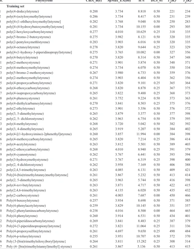
Table 1. Molecular descriptors and Tg data of 107 polystyrenes.
No. Polystyrene ChiA_B(e) SpMax_EA(bo) H7s DLS_01 Tg(K)
a T
g(K) b
Training set
1 poly(4-dodecylstyrene) 0.288 3.734 8.818 0.50 221 234
2 poly(4-(octyloxymethyl)styrene) 0.286 3.734 8.417 0.50 231 239
3 poly[4-(1-ethlhexyloxymethyl)styrene] 0.282 3.768 9.048 0.50 250 283
4 poly[4-(4-hydroxybutoxymethyl)styrene] 0.281 3.734 10.155 0.00 293 305
5 poly(2-hexyloxycarbonylstyrene) 0.277 4.010 10.629 0.25 318 335
6 poly(5-bromo-2-butoxystyrene) 0.275 3.982 8.121 0.50 320 335
7 poly(2-pentyloxymethlstyrene) 0.283 3.903 6.016 0.50 320 335
8 poly(4-octanoylstyrene) 0.278 3.820 9.644 0.25 323 329
9 poly[4-(1-hydroxy-3-piperidinopropyl)styrene] 0.275 3.765 10.082 0.00 327 356
10 poly(4-butyrylstyrene) 0.270 3.820 8.314 0.50 347 348
11 poly(2-methoxystyrene) 0.271 3.901 5.874 0.50 348 371
12 poly(4-methoxymethylstyrene) 0.274 3.734 6.070 0.50 350 334
13 poly(5-bromo-2-methoxystyrene) 0.267 3.980 6.733 0.50 359 376
14 poly(2-methoxymethylstyrene) 0.274 3.903 6.404 0.50 362 356
15 poly(4-propoxycarbonylstyrene) 0.271 3.820 9.101 0.25 365 364
16 poly(4-ethoxycarbonylstyrene) 0.268 3.820 8.878 0.25 367 375
17 poly(4-isopropoxycarbonylstyrene) 0.265 3.822 9.488 0.25 368 373
18 poly(4-phenoxystyrene) 0.261 3.752 9.224 0.50 373 363
19 poly(4-diethylcarbamoylstyrene) 0.270 3.841 8.503 0.25 375 376
20 poly(2-ethylstyrene) 0.273 3.901 5.356 0.50 376 372
21 poly(3, 5-dimethylstyrene) 0.265 3.879 5.377 0.50 377 398
22 poly(2, 5- dichlorostyrene) 0.262 3.963 6.754 0.50 379 395
23 poly(4-methylstyrene) 0.268 3.720 5.042 0.50 382 392
24 poly(3, 4-dimethylstyrene) 0.265 3.919 5.207 0.50 384 402
25 poly(4-[(1-hydroxyimino)-2phenethyl]styrene) 0.260 3.857 11.994 0.00 384 398
26 poly(4-methoxycarbonylstyrene) 0.265 3.820 7.214 0.25 386 414
27 poly(4-acetylstyrene) 0.263 3.812 5.501 0.50 389 403
28 poly(2-ethoxycarbonylstyrene) 0.268 4.010 8.940 0.25 391 379
29 poly(4-cyanostyrene) 0.262 3.767 6.441 0.50 393 394
30 poly(3-hydroxymethystyrene) 0.271 3.767 6.319 0.25 398 400
31 poly(2, 4-dichlorostyrene) 0.262 3.958 7.169 0.50 406 388
32 poly(2,4,5-trimethylstyrene) 0.263 4.085 6.131 0.50 409 421
33 Poly[4-(bis(trimethylstanny)methyl)styrene] 0.261 3.867 5.232 0.50 413 414
34 poly(2, 5-dimethylstyrene) 0.265 3.963 5.744 0.50 416 398
35 poly(4-tert-butylstyrene) 0.263 3.871 4.717 0.50 422 415
36 poly(2,4,6-trimethylstyrene) 0.263 4.135 6.020 0.50 435 432
37 poly(2-carboxystyrene) 0.261 4.003 7.687 0.00 450 466
38 Poly(4-benzoylstyrene) 0.257 3.934 8.698 0.50 371 385
39 Poly(4-phenylacetylstyrene) 0.259 3.829 10.145 0.50 351 357
40 Poly(2-phenylaminocarbonylstyrene) 0.258 4.016 8.500 0.00 464 465
41 Poly(4-phenylstyrene) 0.260 3.914 6.531 0.50 434 401
42 Poly(4-piperidinocarbonylstyrene) 0.269 3.841 8.483 0.25 387 379
43 Poly[4-(3-piperidinopropionyl)styrene] 0.272 3.821 11.064 0.25 311 336
44 Poly(4-propoxysulfonylstyrene) 0.261 4.697 9.650 0.25 490 484
45 Poly(4-p-toluoylstyrene) 0.255 3.951 10.707 0.50 372 370
46 Poly{3-[bis(trimethylsiloxy)boryl]styrene} 0.264 3.811 15.282 0.25 308 314
47 Poly (4- [bis(trimethylstannyl)methyl] styrene) 0.261 3.867 5.136 0.50 413 415
a T
g data were taken from Brandrup et al. [13]; bT
No. Polystyrene ChiA_B(e) SpMax_EA(bo) H7s DLS_01 Tg(K)a T g(K)
b
48 poly(4-hexylstyrene) 0.283 3.734 7.830 0.50 246 252
49 poly[4-(1-hydroxy-1-methylbutyl)styrene] 0.269 3.885 6.338 0.25 403 416
50 poly[4-(1-hydroxy-1-methylhexyl)styrene] 0.273 3.885 10.191 0.25 364 344
51 poly[4-(1-hydroxy-1-methylpropyl)styrene] 0.266 3.884 5.442 0.25 459 441
52 poly(4-ethylstyrene) 0.273 3.733 4.802 0.50 350 355
53 poly(4-nonylstyrene) 0.287 3.734 8.706 0.50 220 236
54 poly(4-tetradecylstyrene) 0.289 3.734 9.289 0.50 237 232
55 poly[4-(2-hydroxybutoxymethyl)styrene] 0.276 3.734 11.064 0.00 319 309
56 poly(5-bromo-2-pentyoxystyrene) 0.277 3.982 7.429 0.50 322 337
57 poly(4-isopentyloxystyrene) 0.275 3.734 8.632 0.50 330 316
58 poly(2-butoxymethylstyrene) 0.281 3.903 6.267 0.50 340 339
59 poly(4-valerylstyrene) 0.273 3.820 8.735 0.50 343 337
60 poly(4-butoxycarbonylstyrene) 0.273 3.820 10.176 0.25 349 344 61 poly(4-methoxy-2-methylstyrene) 0.268 3.965 6.787 0.50 358 371 62 poly(2-isopropoxymethylstyrene) 0.273 3.903 7.998 0.50 361 341
63 poly(4-isobutoxycarbonylstyrene) 0.267 3.821 9.820 0.25 363 363
64 poly(4-fluorostyrene) 0.265 3.720 7.357 0.50 368 376
65 poly(styrene) 0.271 3.622 4.565 0.50 364 356
66 poly(4-propionylstyrene) 0.267 3.820 6.429 0.50 375 377
67 poly(2,3,4,5,6,-pentafluorostyrene) 0.249 4.413 17.543 0.50 378 377
68 poly(4-chlorostyrene) 0.266 3.720 5.821 0.50 383 392
69 poly(2, 4-dimethylstyrene) 0.265 3.958 5.417 0.50 385 402
70 poly(4-bromostyrene) 0.267 3.720 5.249 0.50 391 395
Test set
71 poly(4-chloro-3-fluorostyrene) 0.261 3.919 7.155 0.50 395 388
72 poly(2-isobutoxycarbonylstyrene) 0.268 4.010 7.650 0.25 400 401
73 poly(4-hydroxymethystyrene) 0.271 3.733 5.854 0.25 413 394
74 poly[4-(1-hydroxy-1-methylethyl)styrene] 0.261 3.871 5.408 0.25 438 454
75 poly(4-hexyloxymethystyrene) 0.284 3.734 8.839 0.50 253 249
76 poly(4-propoxymethylstyrene) 0.279 3.734 8.429 0.50 295 284
77 Poly[4-(sec-butoxymethyl)styrene] 0.276 3.734 8.869 0.50 313 309
78 poly(5-bromo-2-propoxystyrene) 0.273 3.982 7.680 0.50 327 345 79 poly(2-butoxycarbonylstyrene) 0.273 4.010 10.353 0.25 339 345
80 poly[2-(2-dimethylaminoethoxycarbonyl)styrene] 0.269 4.010 10.534 0.25 342 352
81 poly(2-ethoxymethylstyrene) 0.277 3.903 7.002 0.50 347 342
82 poly(2-isopentyloxymethylstyrene) 0.277 3.903 6.615 0.50 351 346
83 poly(4-sec-butylstyrene) 0.273 3.764 5.284 0.50 359 365
84 poly(4-methoxystyrene) 0.270 3.733 5.556 0.50 362 374
85 poly(2-pentyloxycarbonylstyrene) 0.275 4.010 9.383 0.25 365 354
86 poly(3-methylstyrene) 0.268 3.752 5.205 0.50 370 394
87 poly(2,5-difluorostyrene) 0.260 3.963 9.602 0.50 374 365
88 poly(2-propoxycarbonylstyrene) 0.271 4.010 8.667 0.25 381 374 89 poly(2-fluoro-5-methylstyrene) 0.263 3.963 8.028 0.50 384 373 90 poly(4-chloro-3-methylstyrene) 0.264 3.919 6.218 0.50 387 390
91 poly(2-chlorostyrene) 0.267 3.880 5.996 0.50 392 382
92 poly(4-dimethylaminocarbonylstyrene) 0.263 3.837 6.944 0.25 398 423 93 poly(2-methoxycarbonylstyrene) 0.265 4.010 7.907 0.25 403 408
94 poly(2-methylstyrene) 0.268 3.880 5.080 0.50 409 392
95 poly(4-hydroxystyrene) 0.266 3.720 6.714 0.25 433 416
96 poly(4-decylstyrene) 0.287 3.734 8.641 0.50 208 236
97 poly(2-isopentyloxycarbonylstyrene) 0.270 4.010 10.984 0.25 341 344
98 poly(5-bromo-2-ethoxystyrene) 0.270 3.982 7.632 0.50 353 355
99 poly(2-hydroxymethystyrene) 0.271 3.901 6.795 0.25 433 402
100 poly(2-octyloxystyrene) 0.285 3.903 6.698 0.50 286 322
101 poly(4-octylstyrene) 0.286 3.734 8.727 0.50 228 239
102 poly(3, 4-dichlorostyrene) 0.262 3.919 6.395 0.50 401 395
a T
g data were taken from Brandrup et al. [13]; bT
2.2 Descriptor computation
A polymeric material consists of a mixture of giant molecules. Therefore, it is impossible to calculate descriptors directly from molecular structures of the polymeric material. Two approaches have been adopted to resolve this problem. One is using the repeating unit to calculate descriptors for the corresponding polymer. The other is using the monomer as representative of the corresponding polymer[1].
Tg is a temperature point used to express transition region, where polymer chain segments can move from frozen to movement (or vice versa). Below the glass transition region, 1-4 chain atoms are involved in motion. Further, these motions are largely restricted to vibrations and short-range rotational motions. During the glass transition region, 10-50 chain atoms attain sufficient thermal energy to move in a coordinated manner. In Tg region, these chain atoms (motion units) are first mobilized before the whole molecule starts moving. On further heating, the increased energy allotted to the chains permits them reptate out through entanglements rapidly and flow as individual molecules[14,15].
The structures of polymer chain segment have an effect on its glass transition and are correlated to Tgs. According to above theory of glass transition, descriptors calculated from the chain segments are more accurate in describing structures affecting polymer Tgs than that from repeating units and monomers. From a theoretical point of view, the chain segment used to calculate descriptors is longer, the descriptors are more accurate in characterizing polymers. The motion units related to glass transition of polymers usually contain 10-50 carbons in length. In addition, a too long segment taken into account may cause difficulty in calculating descriptors, and a too short segment cannot sufficiently represent the structure of motion units. Thus, chain segments with 20 carbons in chain length were used to calculate molecular descriptors for the corresponding polymers.
Polymeric chain segments containing 20 main chain carbons of polystyrenes were first sketched using ChemBioDraw Ultra 11.0 in ChemBioOffice 2008 program. For example, the structure model consisting of 10 repeating units end-capped by two hydrogens (see Figure 1) was adopted as the representative structure of poly(styrene) (No. 65 in Table 1) to calculate the descriptors.
Subsequently, the sketched 2D molecular structures were converted to 3D structures and optimized using a molecular mechanics (MM2 force field) in ChemBio3D Ultra 11.0 with the convergence criterion of minimum rms
of gradient value being 0.01 kcal/molÅ. The optimized molecules were saved in Sybyl mol2 (.mol2) format as the input files for Dragon software[16]. Lastly, 4885 descriptors
were calculated for each energy-minimized motion unit with Dragon software. Descriptors with constant or near constant values and with pair correlation greater than or equal to 0.90 were removed in order to reduce redundant and non-useful information. After excluding redundant and non-useful variables, 551 descriptors were remained to undergo descriptor selection. A relative optimal subset of descriptors was obtained by applying MLR analysis in IBM SPSS Statistics 19.
2.3 Artificial neural network
The optimal descriptors subset was fed to artificial neural network (ANN) as input vectors. ANNs are computational models, which simulate the human brain behavior. The common networks consist of an input layer, some number of hidden layers (intermediate layers) and an output layer. Each layer includes a number of processing nodes, called neurons or units. Each node in the network is inluenced by those nodes to which it is connected in a highly complex and parallel way. The degree of inluence is dictated by the values of the links or connections. Through a training algorithm, the overall behavior of ANNs can be modified by adjusting the weights (or the values of the links or connections). After learning from the input dataset, ANNs acquire knowledge and can be applied on test set data not present in the training set. The output layer produces the prediction values of properties interested. One of the most popular algorithms applied in the training phase is the error back-propagation (BP) algorithm. The number of neurons in the hidden layer shouled be optimized by trial and validation until no obvious improvement was seen for that model[17].
3. Results and Discussions
By analyzing the correlation between the 551 descriptors and Tgs of 70 polystyrenes in the training set with stepwise
MLR analysis in IBM SPSS Statistics 19, Equation 1 and the corresponding statistical results were obtained.
No. Polystyrene ChiA_B(e) SpMax_EA(bo) H7s DLS_01 Tg(K)a T
g(K) b
103 poly(4-hexanoylstyrene) 0.275 3.820 10.423 0.50 339 321
104 poly(2-phenoxycarbonylstyrene) 0.258 4.016 8.596 0.25 397 427 105 poly(2-methaminocarbonylstyrene) 0.266 4.010 7.803 0.00 462 456
106 poly(4-p-anisoylstyrene) 0.257 3.953 10.577 0.25 376 387
107 Poly(2-phenethyloxymethylstyrene) 0.267 3.903 6.696 0.50 336 372
a T
g data were taken from Brandrup et al.[ 13]; bT
g data were calculated with the ANN model.
g 1346.200 4546.871 _ ( )
100.47 _ ( ) 12.653 7 122.231 _ 01
T ChiA B e
SpMax EA bo H s DLS
= − +
− − (1)
n = 70, R = 0.955, R2= 0.912, s = 16.717, F = 167.652
where n is the number of samples from the training set; s is the standard error of estimate; R is the correlation coefficient;
F is the Fischer ratio.
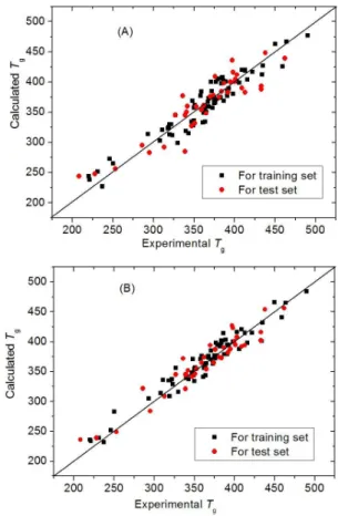
The four molecular descriptors, ChiA_B(e), SpMax_EA(bo), H7s and DLS_01 appearing in above MLR model and the corresponding descriptor values are shown in Table 1. Their descriptor characteristics are listed in Table 2; and their definitions[18] are shown in Table 3. Calculated results with
Equation 1 are depicted in Figure 2A. The rms errors of Tgs of the training and test sets are 16.1 and 22.4 K, respectively.
The four descriptors are then fed to ANN as input vectors. The optimal condition of the neural network was obtained by adjusting various parameters by trial-and-error. The architecture of the final optimum BP neural network is [4-7-1], with the number of hidden layer being 1, the nodes in hidden layer being 7, the permission error being 0.00001, the momentum being 0.6, and the sigmoid parameter being 0.9. The results from ANN method are listed in Table 1 and depicted in Figure 2B, which indicate that the predicted Tg
values are close to the experimental ones. The rms error of training set is 13.6 K (R = 0.939). The test set rms error is 17.1 K (R = 0.902) which is less than the errors from the test
set in previous model (20.5 K)[9]. The mean relative error for
the 107 polystyrenes in Table 1 is 3.4%, less than that from the model of Yu et al.[9] (3.7%). Furthermore, it should be
noted that the test set in this paper possesses 37 polystyrenes, more than the number of samples (11 polystyrenes)[9].
And it is much easier to obtain better results on small test set of polymers. In comparison to previous model on Tgs of polystyrenes[9], the statistic qualities of our model is
accurate and acceptable. Therefore, it is feasible to calculate molecular descriptors from the chain segments of polymer backbones comprising 10 repeating units for developing Tg
model of polystyrenes.
Table 2 shows that each descriptor in Equation 1 has a
Sig.-value near to 0, and less than the default level of 0.05, which suggest that these descriptors are significant for Tgs.
Table 2. Characteristics of descriptors appearing in MLR model.
Descriptors Unstandardized
Coefficients Std. Error
Standardized
Coefficients t Sig. VIF
Constant 1346.200 110.153 12.221
ChiA_B(e) -4546.871 273.430 -0.685 -16.629 0.000 1.249
SpMax_EA(bo) 100.047 14.650 0.288 6.829 0.000 1.309
H7s -12.653 0.959 -0.556 -13.200 0.000 1.307
DLS_01 -122.231 13.833 -0.364 -8.836 0.000 1.247
Table 3. The symbol, class and definition for descriptors appearing in MLR models.
Symbol Class Definition
ChiA_B(e) 2D matrix-based descriptors Average randic-like index from burden matrix weighted by Sanderson electronegativity
SpMax_EA(bo) Edge adjacency indices Leading eigenvalue from edge adjacency matrix weighted by bond order
H7s GETAWAY descriptors H autocorrelation of lag 7 / weighted by I-state
DLS_01 Drug-like indices Modified drug-like score from Lipinski (4 rules)
Figure 2. Plots of calculated vs. experimental Tg values of polystyrenes: (A) for MLR model; (B) for ANN model. Moreover, all variance inflation factor (VIF) values are less than 2, far less than the default value of 10. Thus these descriptors are “pure” without “mixing” or contamination from other descriptors, and each descriptor relects some particular molecular structures affecting Tgs.
According to the t-test, the most significant descriptor in the MLR model is ChiA_B(e) (2D matrix-based descriptors)[16].
Chi_M(e) ChiA_B(e)
nBO
= (2)
Where nBO is the number of graph edges. Chi_M(e) is the Randic-like index calculated by applying Sanderson electronegativity as the vertex weighting scheme and a H-depleted molecular graph as a square matrix:
1/ 2 1
1 1
Chi_M(e) nSK nSK ij i( ; ) j( ; )
i j i
VS M e VS M e
− −
= = +
= ∑ ∑ α ⋅ ⋅ (3)
Here nSK means the number of graph vertices; VSi(M) is the ith matrix row sum; αij are the elements of the adjacency
matrix, which are equal to one for pairs of adjacent vertices, and zero otherwise. ChiA_B(e) reflects information about interatomic distances, bond distances, ring types, planar and non-planar systems and atom types[16]. A small ChiA_B(e)
indicates a small interatomic distances, which results in a low degree of freedom for rotation and leads to high Tg.
The second significant descriptor is the GETAWAY (GEometry, Topology, and Atom-Weights AssemblY) descriptor, H7s (H autocorrelation of lag 7 / weighted by I-state). The descriptor H7s encodes information on structural fragments, such as the effective position of substituents and fragments in the molecular space, and accounts information on molecular size and shape as well as for specific atomic properties[16]. A large H7s suggests that a polymer has a large
side group, which decreases the volume ratio of phenyl ring to other substituent groups. While the aromatic or cyclic structure in bulky side groups increases rotational barrier for backbone chain and leads to high Tg. Therefore, a polymer with large H7s may have a low Tg.
The next significant descriptor is the Drug-like indice DLS_01. The descriptor DLS_01, being modified drug-like score from Lipinski (4 rules), is calculated as 1 minus Lipinski Alert Index (LAI), while LAI is defined as the ratio between the number of satisfied conditions over the total number of conditions, i.e., (1) there are more than 5 H-bond donors; (2) there are more than 10 H-bond acceptors (N and O atoms); (3) molecular weight (MW) is over 500; and (4) Moriguchi’s logP (MLogP) is over 4.15[16].
DLS_01 is related to the number of intermolecular hydrogen bonds, which increase intermolecular force and determine the magnitude of molecular aggregates. Polymer molecules with small DLS_01 hold together more strongly due to intermolecular hydrogen bonds and are unable to mover that easily, and possess high Tgs.
According to the t-test, the last significant descriptor in the MLR model is SpMax_EA(bo). Edge adjacency index, SpMax_EA(bo), is derived from the H-depleted molecular graph and encodes the connectivity between graph edges. It is leading eigenvalue from edge adjacency matrix weighted by bond order. SpMax_EA(bo) reflects molecular shape and implies the substituent position in the phenyl ring for styrenes[16]. Compared to styrenes with
substituents lying in p-or m-positions of the phenyl ring, a styrene with a substituent lying in o-positions usually has a larger SpMax_EA(bo), which can be seen from Table 1. The substituents in o-positions will enhance rotational barrier
for backbone chain, increase rigidity of polymer chains and result in higher Tgs[9].
Despite a variety of factors affecting the Tg values of polymeric materials, intermolecular forces and molecular flexibility (or rigidity) are two important factors related to Tgs. The descriptor DLS_01 reflects the intermolecular
forces, while descriptors ChiA_B(e), SpMax_EA(bo) and H7s indicate the stiffness of polymer. Therefore, the four descriptors can predict Tgs sufficiently.
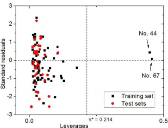
Figure 3 (Williams plot) was obtained to visualize the applicability domain of the ANN model in this paper. According to Williams plot based on standardized residuals vs. leverages, predictions for only those samples that fall into this domain may be considered reliable[19,20]. Figure 3 shows that only
the two samples No. 44, poly(4-propoxysulfonylstyrene) and No. 67, poly(2,3,4,5,6,-pentafluorostyrene) in the training set have larger leverage h values (0.448 and 0.456, respectively), greater than the warning leverage
h* (= 0.214). But their standardized residual values (0.430 and 0.075, respectively) are less than 3. Thus the two samples, poly(4-propoxysulfonylstyrene) and poly(2,3,4,5,6,-pentafluorostyrene), can stabilize the ANN model of polystyrenes and make it more accurate.
4. Conclusions
Four molecular descriptors calculated from the chain segments of main chains comprising 10 repeating units were adopted for developing QSPR model of Tgs for polystyrenes. MLR analysis was used to select the optimal subset of descriptors after molecular descriptor generation for each chain segment. The developed ANN model was proved to be accurate and acceptable, with the absolute mean errors for the whole data set is 3.4%, which is less than that of the model published in the literature, although our model possesses more samples for the test set. Therefore, it is feasible calculating molecular descriptors from the chain segments comprising 10 repeating units in length to develop ANN model of Tgs for polystyrenes.
5. Acknowledgements
The project was supported by the National Natural Science Foundation of China (No. 21472040) and Scientific Research Fund of the Hunan Provincial Education Department (No. 16A047).
6. References
1. Katritzky, A. R., Kuanar, M., Slavov, S., Hall, C. D., Karelson, M., Kahn, I., & Dobchev, D. A. (2010). Quantitative correlation of physical and chemical properties with chemical structure: utility for prediction. Chemical Reviews, 110(10), 5714-5789. PMid:20731377. http://dx.doi.org/10.1021/cr900238d. 2. Bicerano, J. (1996). Prediction of polymer properties. 2nd ed.
New York: Marcel Dekker.
3. Karelson, M., Lobanov, V. S., & Katritzky, A. R. (1996). Quantum-chemical descriptors in QSAR/QSPR studies.
Chemical Reviews, 96(3), 1027-1044. PMid:11848779. http://
dx.doi.org/10.1021/cr950202r.
4. Van Krevelen, D. W. (1976). Properties of polymers their estimation and correlation with chemical structure. 2nd ed. New York: Elsevier.
5. Joyce, S. J., Osguthorpe, D. J., Padgett, J. A., & Price, G. J. (1995). Neural network prediction of glass-transition temperatures from monomer structure. Journal of the Chemical Society, Faraday Transactions, 91(16), 2491-2496. http:// dx.doi.org/10.1039/ft9959102491.
6. Katritzky, A. R., Rachwal, P., Law, K. W., Karelson, M., & Lobanov, V. S. (1996). Prediction of polymer glass transition temperatures using a general quantitative structure-property relationship treatment. Journal of Chemical Information and Computer Sciences, 36(4), 879-884. http://dx.doi.org/10.1021/ ci950156w.
7. Katritzky, A. R., Sild, S., Lobanov, V., & Karelson, M. (1998). Quantitative Structure-Property Relationship (QSPR) correlation of glass transition temperatures of high molecular weight polymers. Journal of Chemical Information and Computer Sciences, 38(2), 300-304. http://dx.doi.org/10.1021/ci9700687. 8. Cao, C., & Lin, Y. (2003). Correlation between the glass transition temperatures and repeating unit structure for high molecular weight polymers. Journal of Chemical Information and Computer Sciences, 43(2), 643-650. PMid:12653533.
http://dx.doi.org/10.1021/ci0202990.
9. Yu, X. L., Wang, X. Y., Li, X. B., Gao, J. W., & Wang, H. L. (2006). Prediction of glass transition temperatures for polystyrenes by a four-descriptors QSPR model. Macromolecular Theory
and Simulations, 15(1), 94-99. http://dx.doi.org/10.1002/ mats.200500057.
10. Liu, A. H., Wang, X. Y., Wang, L., Wang, H. L., & Wang, H. L. (2007). Prediction of dielectric constants and glass transition temperatures of polymers by quantitative structure property relationships. European Polymer Journal, 43(3), 989-995. http://dx.doi.org/10.1016/j.eurpolymj.2006.12.029. 11. Liu, W. Q., Yi, P. G., & Tang, Z. L. (2006). QSPR models for
various properties of polymethacrylates based on quantum chemical descriptors. QSAR & Combinatorial Science, 25(10), 936-943. http://dx.doi.org/10.1002/qsar.200510177. 12. Yu, X. L., Yi, B., Wang, X. Y., & Xie, Z. M. (2007). Correlation
between the glass transition temperatures and multipole moments for polymers. Chemical Physics, 332(1), 115-118. http://dx.doi.org/10.1016/j.chemphys.2006.11.029. 13. Brandrup, J., Immergut, E. H., & Grulke, E. A. (1999). Polymer
handbook. 4th ed. New York: Wiley-Interscience.
14. Sperling, L. H. (1992). Introduction to physical polymer science. New York: John Wiley & Sons.
15. Gedde, U. W. (1995). Polymer physics. London: Chapman &
Hall.
16. Talete SRL. (2012). Dragon: software for molecular descriptor calculation. Version 6.0. Milano: Talete SRL. Retrieved in 20
February 2016, from http://www.talete.mi.it/
17. Yu, X. L., Yi, B., Liu, F., & Wang, X. Y. (2008). Prediction of the dielectric dissipation factor tan δ of polymers with an ANN model based on the DFT calculation. Reactive & Functional Polymers, 68(11), 1557-1562. http://dx.doi.org/10.1016/j.
reactfunctpolym.2008.08.009.
18. Todeschini, R., & Consonni, V. (2009). Molecular descriptors for chemoinformatics. Weinheim: Wiley-VCH. 2 v. 19. Tropsha, A., Gramatica, P., & Gombar, V. K. (2003). The
importance of being earnest: validation is the absolute essential for successful application and interpretation of QSPR Models.
QSAR & Combinatorial Science, 22(1), 69-77. http://dx.doi. org/10.1002/qsar.200390007.
20. Wang, Y. N., Chen, J. W., Li, X. H., Wang, B., Cai, X. Y., & Huang, L. P. (2009). Predicting rate constants of hydroxyl radical reactions with organic pollutants: algorithm, validation, applicability domain, and mechanistic interpretation. Atmospheric Environment, 43(5), 1131-1135. http://dx.doi.org/10.1016/j.
atmosenv.2008.11.012.