397
Abstract
Drilling and stabilizing oil wells are important technological challenges for devel-oping the Brazilian Pre-Salt deposits due to creep behaviour of salt rocks, which results in well closure and collapse. The objectives of this work are to analyse the currently used creep models and to propose a new empirical model that comprehends the three creep stages. This work suggests that a deep interpretation of Burger’s rheological model, based on the physical parameters of creep phenomenon, should be investigated. The problem of the explicit presence of time in creep strain rate models is discussed. The new proposed model is able to reproduce models that describe the transient and the steady-state creep stages. However, its calibration should be careful, based on data from all these creep stages.
Keywords: salt rock, oil drilling, creep models, rock mechanics.
Resumo
A perfuração e a estabilidade dos poços são importantes desaios tecnológicos para o desenvolvimento da província petrolífera do Pré-Sal brasileiro, graças à lu-ência das rochas evaporíticas, que provoca o fechamento e o colapso dos poços de pesquisa e de produção. Os objetivos desse trabalho são a análise dos modelos de luência atualmente utilizados e a proposta de um novo modelo empírico, que com-preenda todas as fases da luência. É proposto que uma melhor interpretação do modelo reológico de Burger, baseada nos mecanismos físicos que regem a luência, seja investigada. Uma discussão sobre o problema da presença explícita do tempo na formulação da taxa de deformação por luência é revista. O novo modelo proposto é capaz de replicar modelos que representam a luência primária e secundária, porém sua calibração deve ser criteriosa, com dados de todas essas fases da luência.
Palavras Chave:evaporitos, poços de petróleo, luência, mecânica de rochas.
Gabriel Esteves Motta
Federal University of Minas Gerais Belo Horizonte – Minas Gerais - Brazil [email protected]
Cláudio Lúcio Lopes Pinto
Federal University of Minas Gerais Belo Horizonte – Minas Gerais – Brazil [email protected]
New constitutive
equation for salt rock creep
Novo modelo constitutivo
para fluência de rochas evaporíticas
Mining
Mineração
1. Introduction
The Brazilian Pre-Salt is the biggest oil discovery in last ifty years. Made public in 2007, it could include Brazil among the biggest oil producers in the world. The reservoir is in a 3-4 km thick porous rock layer, under 1.5-3.0 km of seawater and a salt rock layer with up
to 2.5 km of thickness (Riccomini et
al., 2012).
The drilling and stability of oil wells are some of the most important technological challenges for the Brazilian
Pre-Salt development. Creep behaviour of salt rocks causes serious issues to the drilling and stabilizing of oil wells. Clo-sure and collapse due to wall convergence are constantly reported (Urai et al., 2008; Mackay et al., 2007; Ferro et al., 2009).
Creep behaviour has been largely studied for the development of potash mines (Pinto, 1995), oil and gas well drilling (Mackay et al., 2007; Poiate et al., 2006) and nuclear waste disposal (Yao, 2007). Many constitutive
equa-tions, of empiric or rheological nature, have been proposed to describe the creep time-dependent strain (Pinto, 1995; Jae-ger et al., 2007; Grainger, 2012) but all of them have their limitations regarding the physical meaning of the phenomenon.
In this paper, the physical and mathematical hypotheses of salt rock’ constitutive models are investigated and a new empirical model, which comprehends the whole phenomenon, is proposed.
398 REM: R. Esc. Minas, Ouro Preto, 67(4), 397-403, oct. dec. | 2014
Creep behaviour
The ideal time dependent strain behaviour was proposed by Jaeger (2007) and is shown in igure 1.
Upon the application of a stress, an evaporite undergoes transformation to
through an instantaneous elastic strain (A). The strain continues to increase with a decreasing rate in zone I, deined as primary or transient creep. The strain rate goes down to a minimum value,
which holds constant in zone II, deined as secondary or steady-state creep. Zone III represents a theoretical tertiary phase of creep, in which the strain rate increases until material failure (Cruz, 2003).
Figure 1
Theoretical curve of creep for constant de-viatoric stress (adapted from Cruz, 2003)
In stress relief, the behaviour of material should follow path PRQ in zone I, without residual strain, and
path TU V in zone II, where there will be some residual strain (Jaeger et al., 2007).
An adequate equation to describe the curve in Figure 1, as a function of the time, would be described as (1):
(1)
(2)
(3)
(4)
(5)
(6) Here εe represents the elastic strain
and ε1(t), ε2(t) and εe(t) represents
tran-sient, steady-state and tertiary creep, respectively. The strain rate in each zone
would be:
ε = ε
e+
ε
1(t) +
ε
2(t) +
ε
3(t)
∂
2ε
1
(
t
)
∂
t
2<
0
∂
2ε
2
(
t
)
∂
t
2=
0
∂
2ε
3
(
t
)
∂
t
2> 0
Therefore, satisfying the conditions in equations (2), (3) and (4), any function could represent this model, providing a smooth transition from one creep stage to
another. These considerations imply that the total strain is the sum of elastic and creep strain. Experimental results show that the main variables that influence
creep behaviour are temperature (T) and deviatoric stress (σdev), not the hydrostatic
stress (Jaeger et al., 2007; Grainger, 2012). The total strain would be given by:
ε = σ
dev2G
+
ε
CR(
σ
dev,T,t)
This paper will classify the creep models in two categories: the empirical and the rheological ones.
Empirical models
The empirical models aim to it the proposed functions to experi-mental data based or not in physical assumptions about the phenomena
mechanisms.
The most used empirical model for modelling rock creep is the Norton Pow-er Law, proposed in 1929 (Pinto, 1995;
Yao, 2007; Cruz, 2003). It represents a constant strain rate, characteristic of the secondary creep, as shown in the following equation:
399
Here A and n are material param-eters and σ is the deviatoric stress. The model is not capable of representing the primary creep (Pinto, 1995).
The Double Mechanism Law, developed with data from Taquari-Vassouras basin in Northeast of Brazil, has the same form of the Norton Power
Law, with a term that considers tem-perature effect and a stress threshold (σ0) (Grainger, 2012):
ε
.
CR=
[ ( ) e ]
ε
0σ
n 0Q RT
Q RT
-σ
n dev0 (7)
(8)
(9)
(10)
(11)
(12) The temperature term considers the
Arrhenius Law (Yao, 2007), Q represents the activation energy, R is the universal gas constant and T0 is a temperature of reference. The term ε0 represents a
material parameter and σ0 is a stress
threshold: above σ0 or below σ0 different
values of n are used, according to differ-ent creep mechanisms. This equation is useful for complex modelling and where changes in temperature are signiicant. Nevertheless, it fails to represent a truly
transient creep.
The Bayle-Norton Law, or Time Hardening Law, uses a time dependent term to represent the decreasing strain rate in primary creep, as shown in the following equation:
ε
.
CR= A
σ
nt
mwhere m is a new hardening parameter that should be smaller than zero (Pinto, 1995) . However, the Bayle-Norton cannot provide a smooth transition to
secondary creep and the strain rate is ininite for t = 0. Thus, it is necessary to ix a positive initial time. The equation also shows that for increasing values of
time, the Bayle-Norton Law tends to a horizontal straight line that represents steady-state creep instead of presenting a positive inclination.
Rheological models
One-dimensional rheological mod-els deine the materials as idealized
ele-ments, as springs and dashpots (Grainger, 2012) . The most complete rheological
model is the Burger’s substance, whose equation is:
σ
η
1..
ε +
k
1..
ε
=
η
1..
..
k
2k
2k
1k
1σ
+ ( 1+ + )
η
1σ
+
η
2η
2This differential equation is able to reproduce primary and secondary creeps,
according to the equation (6) solved for constant stress:
σ
0k
2η
2ε
(t) =
σ
0k
1σ
0+
[ 1 - e
+
k
η1 t
1
]
t
The model presents the instanta-neous, time independent, elastic strain term, the second term that represents an exponential decreasing strain rate, repre-senting primary creep, and a third linear, time dependent term, which represents
secondary creep.
Rheological models are not used often in salt creep problems because they are not directly related to the creep mechanisms . However, they can provide mathematical background to the physical
models. In addition, only the rheological models provide terms (time differentials of stress and strain) that consider stress and strain variations. The constants of Burger’s model should be interpreted in terms of rock parameters.
Presence of time parameter in creep equations
For all creep models, the strain is an explicit function of the time. The strain rate, according to the ideal model in Fig. 1, varies along the time. Physi-cally, however, the variations should not
be due to the time itself, but to changes in the characteristics of the material and in the environment. It can make it im-possible to be used in every day models where different parts are submitted to
deviatoric stresses at different moments. Some attempts to avoid the explicit use of time have been made, like the Strain Hardening Law (Pinto, 1995; Yao, 2007) [6, 7]:
where εdev is the deviatoric strain and α < 0 is a parameter of the
mate-rial. This model has a mathematical singularity for zero deviatoric strain.
Pinto (1995) proposed a new model that solved the problem:
ε
.
CR=
A
σ
dev n(
γ + ε
dev)
βIn equation (12), A, n, β and γ are material parameters, εdev and σdev are deviatoric strain and stress,
respec-ε
.
CR= A
σ
nε
α400 REM: R. Esc. Minas, Ouro Preto, 67(4), 397-403, oct. dec. | 2014
tively. The equation would guarantee a smooth transition from primary creep
(εdev >> γ) to secondary creep (εdev << γ)
(Pinto, 1995) . However, during primary
creep, small strains occurs, characterizing model similar to the Norton Power Law:
dev
A
σ
n(
γ + ε
dev)
βlim
σ
ndev
=
A’
→
A’ =
A
γ
βε→0
(13)(14)
(15)
(16) For higher strain values, the model turns into a horizontal asymptote:
dev
A
σ
n(
γ + ε
dev)
βlim
= 0
ε→∞
Therefore, the equation proposed by Pinto (1995) represents a truly time
hardening material, achieving inite strain rates for small strain values. The equation
depends only in material parameters, without explicit time dependence.
Proposing a new creep constitutive equation
A new empirical model would have two objectives: comprehend the three creep stages and eliminate any explicit function of the time in the strain rate
formulations. Following the structure of equation (1), the equation proposed by Pinto (1995) could be used as a primary creep term and the Double Mechanism
Law could be used as a secondary creep term. The tertiary creep would be an in-creasing function of the deviatoric strain. One resulting equation could be:
dev dev
A
3σ
n devA
1σ
n(
γ + ε
dev)
βε
.
cr=
1
[ ( ) e ]
ε
0σ
n 0Q RT
Q RT
-σ
n dev22
0 3
ε
n3
+
+
Due to the large number of param-eters, some arbitrary simpliications will be made. First, n1 = n2 = n3 = n, which means that the stress will have the same
inluence in all creep stages. Then, the temperature will be considered as well to have the same inluence in all three creep stages. Due to lack of data, the
stress threshold of the Double Mecha-nism Law will not be considered as well. Thus, the new constitutive model will be expressed as:
dev
A
3ε
nA
1A
2
(
γ + ε
dev)
βε
.
cr=
σ
ndev
e
Q RT
Q RT
-0
+
+
[ ]
The equation have seven material parameters (A1, A2, A3, γ, β,α and n). Q is the activation energy, R is the universal constant of the gases, T0 is a
reference absolute temperature and T is the absolute temperature of the system.
εdev and σdev are the deviatoric
strain and stress, respectively.
The equation should be calibrated with data from all three creep stages of the material are necessary.
Two-dimensional modelling
The equation was tested with the rock mechanics software FLAC 2D, from ITASCA, which utilizes a FDM/ FVM (Finite Differences/Finite Volumes Method) algorithm (Cruz, 2003) .
The software has a programming tool, FISH language, which allows the user to implement new constitutive models. More information about it can be found in Pinto (1995) and in FLAC
user’s manual (ITASCA, 2006).
This work considers the von Mises deviatoric stress and strain as a measure of the magnitude of the distortion stresses.
2. Methodology
The element grid utilized in the tests is shown in igure 2.
The grid’s intent is to simulate a well closure due to convergence of the wall.
Figure 2
401
The well radius was considered to be 0.108 m, according to Mackay (2007) . The model extends until 1.08 m in order to minimize the excavation ends effects in the stresses and strain on the external border of the model. The grid has 10 cells in the radial direction and 50 cells in the tangential direction. Each cell length in the radial direction is 10% bigger than its predecessor.
The objective of the tests is to verify the ability of the new model to adhere to different models considering different materials.
The regions x = 0 and y = 0 were considered symmetry borders (no
dis-placement allowed in the perpendicular direction) and a horizontal stress of 47 MPa (compressive stress) was applied in the external borders (x = 1.08 and y = 1.08). This stress considered a 2,000 m thick water layer (ρ = 1,000 kg/m3) and a
1,000 m thick sediment layer (ρ = 2,700 kg/m3), conditions at the top of the salt
layer in Brazilian Pre-Salt (Poiate et al., 2006) . The initial vertical stress was set to 47 MPa as well, as the evaporite materials only attain equilibrium in hy-drostatic stress conditions (Pinto, 1995) . The tests considered two differ-ent materials: halite and taquidrite, evaporites present in the salt layer of
Santos and Campos basins (Mackay et
al., 2007) .
The simulations were performed in three steps: irst, the border of the well was ixed and the in situ stress conditions were calculated. Then, the border of the well was liberated and a new stage of equilibrium was attained without creep inluence, which means that the elastic equilibrium was considered to be in-stantaneous. The last step was the creep displacement calculations stage, until the end time of 3014 days, approximately 8.5 years.
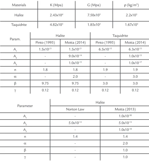
The parameters used in the tests are shown in the tables 1, 2 and 3.
Materials K (Mpa) G (Mpa) ρ (kg/m3)
Halite 2.43x10⁴ 7.50x10³ 2.2x10³
Taquidrite 4.82x10³ 1.85x10³ 1.67x10³
Table 1 Physical parameters of the materials used in the simulations
Table 2 Parameters for the simulations comparing the new model to Pinto’s model
Table 3 Parameters for the simulations comparing the new model to Norton Power Law
Param. Halite Taquidrite
Pinto (1995) Motta (2014) Pinto (1995) Motta (2014) A1 1.5x10⁻²¹ 1.5x10⁻²¹ 6.5x10⁻¹⁵ 6.3x10⁻¹⁵
A2 - 9.0x10⁻¹⁴ - 1.0x10⁻¹³
A3 - 1.0x10⁻¹⁵ - 1.0x10⁻¹⁷
n 1.8 1.8 1.9 1.9
α - 2.0 - 3.0
β 9.75 9.75 3.0 3.0
γ 0.12 0.12 0.12 0.12
Parameter Halite
Norton Law Motta (2013)
A1 - 1.0x10⁻³⁰
A2 5.0x10⁻¹³ 5.0x10⁻¹³
A3 - 1.0x10⁻¹⁸
n 1.4 1.4
α - 2.0
β - 1.0
γ - 1.0
The same density and the elastic parameters, shear modulus (G) and bulk modulus (K), were used in all tests. The parameters for Pinto’s model and Norton Power Law were obtained from Cruz (2003) and consisted of
data from Taquari-Vassouras basin, in the Northeast of Brazil. The param-eters of the new model were deined in order to attain as close as possible to the correspondent parameters in the other models.
As the new model has more rameters than the others do, these pa-rameters were set to have small values. When the linear (Ai) parameters have small values, the power (Greek letters) do not have considerable inluence.
3. Results
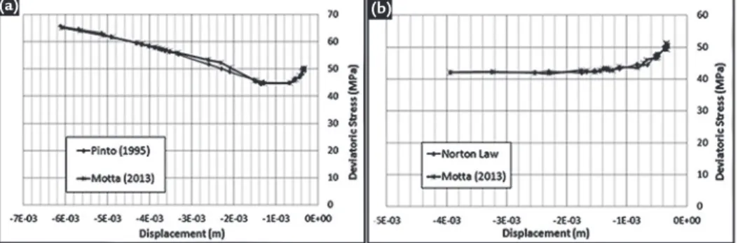
Figure 3 shows radial displacement of the well border as function of the creep time for the two materials.
The plotted data from different models show completely different be-haviours:
402 REM: R. Esc. Minas, Ouro Preto, 67(4), 397-403, oct. dec. | 2014
(a)
Figure 3
Displacement versus creep time: comparison between
(a) the new model
and Pinto’s model with halite; (b) the new model and Pinto’s model with taquidrite; (c) the new model and Norton Power Law with halite
The results show that the new model showed a good adherence to the two dif-ferent models that represent two differ-ent creep stages. The closer the models’ parameters are, the closer the curves. A difference of 0.2 in the A1 parameter for the taquidrite test resulted in a slight dif-ference between the curves.
The additional parameters of the new model, set up as minimum, did not inluenced the result; these parameters could be excluded when the creep stage that they do represent are not of interest: the model could be reduced to Pinto’s model with no loss.
Figure 4 shows the deviatoric stress
in the border of the well versus the creep displacement.
The new model reproduces the stress behaviour deined by both Pinto’s model and Norton Power Law. The difference observed in Pinto’s model comparison can be assigned to a restricted increase in the unbalanced force.
Figure 4 Deviatoric stress
at the well borders (with halite): (a) comparison between
the new model and Pinto’s model; (b) comparison between
the new model and Norton Power Law
(a) (b)
It is interesting to observe that none of the models provides a systematic de-crease in the deviatoric stress due to strain. As creep strain occurs only at the presence of a deviatoric stress, it should provide a stress relief on the rock mass (Pinto, 1995) . Pinto’s model returns an increasing deviatoric stress after a minimum value
and Norton Power Law shows a static deviatoric stress for high time intervals. In both cases, creep strain would occur indeinitely. The new model will not solve this problem, as it reproduces exactly the same stress behaviour as the others. Therefore, none of the models should be used for extrapolation.
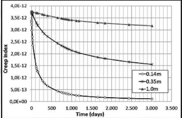
In Pinto’s model, the strain rate is a function of deviatoric strain and deviatoric stress. The deviatoric strain is responsible for determining the inluence of the rial in the strain rate: the more the mate-rial is distorted, the higher is the rate of distortion. One can deine a ‘creep index’ according to:
A’ =
A
1(
γ + ε
dev)
β(17)
The deined creep index (A’) would reduce as the deviatoric stress increases, characterizing the primary creep. If the creep index was a function of time, its value would be constant for every region of the model, as the time passes equally in every point of the model. Figure 5 shows
that A’ value is different in different re-gions of the model, as the material suffer different inluences from the excavation.
It is possible to see that the more distant from the centre of the excavation, the higher is its creep index. This can be assigned to the lower deviatoric strain
ob-served at distant points. If the creep index was a function of time (as in Bayle-Norton Law, for example) the three curves would superpose each other. It is worth mention-ing that the horizontal asymptote y = 0 observed in the 0.14m curve, agrees with the mathematical analysis.
(a) (b)
403
Received: 29 August 2014 - Accepted: 3 October 2014. Figure 5
Creep index (A’) behaviour: creep strain rate decrease with time
4. Conclusions
The analysis of the empirical models showed that none of the ones proposed in the literature comprehends more than one creep stage, and some of them have mathematical problems with small time and strain values. Empirical equations should not be used to extrapo-lation problems. This work suggests a deeper interpretation of the physical
meaning of the Burger’s model, in order to solve the mathematical problems of the empirical models.
The discussion about the problem of the strain rate as an explicit function of time was demonstrated by the results, which showed different creep strain rates in different regions of the model. As the time passes equally all around the model,
it should not directly deine the strain rate of the material.
The new model was able to re-produce the behaviour of two different creep models that represent two distinct creep stages. However, the new equation requires a careful calibration due the larger number of parameters. Data from all creep stages are needed.
5. References
CRUZ, E.R. Modelagem numérica de escavações subterrâneas em evaporitos da sub--bacia de Taquari-Vassouras. Belo Horizonte: Escola de Engenharia da UFMG, 2003. 86p. (Dissertação, Mestrado, Tecnologia Mineral)
FERRO, F., TEIXEIRA, P. Os desaios do Pré-Sal. Brasília: Câmara dos Deputados, Edições Câmara, 2009. 78 p. – (Série cadernos de altos estudos, n. 5)
GRAINGER, P. A. M. Numerical analysis of the mechanical behavior of cement she-aths in wells through Salt Formations. Rio de Janeiro: Pontifícia Universidade Ca-tólica do Rio de Janeiro, 2012. 134p. (Dissertação, Mestrado, Engenharia Civil) ITASCA CONSULTING GROUP, INC. Fast Lagrangian Analysis of Continua;
User’s Guide. 3 ed. Minneapolis, 2006.
JAEGER, J. C., COOK, N. G. W., ZIMMERMAN, R. W. Fundamentals of rock
mechanics. 4 ed. Oxford: Blackwell Publishing, 2007. 475p.
MACKAY, F., BOTELHO, F. V. C., INOUE, N., FOUNTOURA, S.A.B. Analyzing geomechanical effects while drilling salt wells through numerical modelling. In: ABAQUS USER’S CONFERENCE, 19; Paris, 2007.
PINTO, C. L. L. Longwall mining in Boulby Potash Mining: a numerical study. Gol-den: Colorado School of Mines, 1995. 226p. (Thesis, Doctor of Philosophy, Mi-ning Engineering)
POIATE, E., DA COSTA, A. M., FALCAO, J. L. DRILLING BRAZILIAN SALT-1: Petrobras studies salt creep and well closure. Oil and Gas Journal. v.104,n. 21; 36-45, May 2006.
RICCOMINI, C., SANT’ANNA, L. G., TASSINARI, C. C. G. Pré-Sal: geologia e exploração. Revista USP, São Paulo, n. 95, p. 33-42, set./out./nov. 2012.
URAI, J. L., SCHLEDER, Z., SPIERS, C. J., KUKLA, P. A. Flow and transport pro-perties of salt rocks. In: LITTKE, R., BAYER, U., GAJEWSKI, D., NELSKAMP, S. (Eds.). Dynamics of Complex Intracontinental Basins: The Central European Basin System. Berlin: Springer, 2008. 550p.