doi: 10.1590/0101-7438.2015.035.03.0577
A SIMULATION-BASED METHODOLOGY FOR PREDICTING FOOTBALL MATCH OUTCOMES CONSIDERING EXPERTS’ OPINIONS:
THE 2010 AND 2014 FOOTBALL WORLD CUP CASES
Francisco Louzada
1*, Adriano K. Suzuki
1, Luis E.B. Salasar
2,
Anderson Ara
2and Jos´e G. Leite
2Received January 10, 2014 / Accepted September 11, 2015
ABSTRACT. In this paper we propose a simulation-based method for predicting the 2010 and 2014 Football World Cup. Adopting a bayesian perspective, we modeled the number of goals of two oppos-ing teams as a Poisson distribution whose mean is proportional to the relative technical level of opponents. FIFA ratings were taken as the measure of technical level of teams and experts’ opinions about scores of matches were taken to construct prior distribution of parameters. Just before each round, tournament simulations were performed in order to estimate probabilities of events of main interest for audience and bettors such as qualifying to the knockout stage, reaching semi-finals, reaching the final match, winning the tournament, among others.
Keywords: Bayesian inference, Football World Cup, forecasting, poisson distribution, simulation.
1 INTRODUCTION
The World Cup tournament (WCT) organized by FIFA (F´ed´eration Internationale de Football Association, French for International Federation of Football Association) is the most important international football championship, which occurs every four years. The first tournament took place in Uruguay in 1930 with 13 invited countries and Uruguay became the first champion. In the current format, the competition gathers 32 teams, the host nation(s) has a guaranteed place and the others are selected from a qualifying phase which occurs in the three-year period preceding the tournament.
The tournament is composed by agroup stagefollowed by aknockout stage. In thegroup stage, the teams play against each other within their group and the top two teams in each group advance
*Corresponding author.
1Departamento de Matem´atica e Estat´ıstica, ICMC, Universidade de S˜ao Paulo, 13566-590 S˜ao Paulo, SP, Brasil. E-mails: [email protected]; [email protected]
to the next stage. In theknockout stage, 16 teams play one-off matches in a single-elimination system, with extra time of 30 minutes (divided in 2 halves of 15 minutes each) and penalty shootouts used to decide the winners when necessary.
In the literature, several articles are directed to football prediction, mostly applied to champi-onship leagues. Keller (1994) has fitted the Poisson distribution to the number of goals scored by England, Ireland, Scotland and Wales in the British International Championship from 1883 to 1980. Lee (1997) also considers the Poisson distribution, but allows for the parameter to de-pend on a general home-ground effect and individual offensive and defensive effects. Karlis & Ntzoufras (2009) applied the Skellam’s distribution to model the goal difference between home and away teams. The authors argue that this approach does not rely neither on independence nor on the marginal Poisson distribution assumptions for the number of goals scored by the teams. A bayesian analysis for predicting match outcomes for the English Premiere League (2006-2007 season) is carried out using a log-linear link function and non-informative prior distributions for the model parameters.
Taking another approach, Brillinger (2008) proposed to model directly the win, draw and loss probabilities by applying a trinomial regression model to the Brazilian 2006 Series A champi-onship. By means of simulation, it is estimated for each team the total points, the probability of winning the championship and the probability of ending the season in the top four places.
To model the number of goals scored by teams in each match, Baio & Blangiardo (2010) pro-poses a Bayesian hierarchical model, while Koopman & Lit (2015) assumes a bivariate Poisson distribution with intensity coefficients that change stochastically over time. Whereas Louzada et al. (2014) assumes a univariate Poisson distribution and consider linear models that express the sum and the difference of goals scored in terms of covariates. Moreover, Alves et al. (2011) propose logit models for the probability of winning football games, Calˆoba & Lins (2006) assess the performance of soccer teams in Brazil using DEA, Dobson & Goddard (2003) provided a a Monte Carlo analysis of the persistence in sequences of football match results, Koning et al. (2003) provides a simulation model for football championships, Scarf & Shi (2008) determines the importance of a match in a tournament, and Sant’Anna (2008) proposes to classify Brazilian soccer clubs by considering rough sets analysis with antisymmetric and intransitive attributes.
In spite of the vast literature directed to League Championship prediction, few articles concern score predictions for the WCT (Dyte & Clarke, 2000; Volf, 2009; Suzuki et al., 2009; Bastos & da Rosa, 2013). Probably, the shortage of researches on the WCT is due to the limited amount of valuable data related to international matches and also to the fact that few competitions confronts teams from different continents.
teams are modeled via a semi-parametric multiplicative regression model of intensity. The au-thor has applied his model to the analysis of the performance of the eight teams that reached the quarter-finals of the 2006 WCT. Suzuki et al. (2009) proposed a bayesian methodology for pre-dicting match outcomes using experts’ opinions and the FIFA ratings as prior information. The method is applied to calculate the win, draw and loss probabilities for each match and also to es-timate classification probabilities in group stage and winning tournament chances for each team on the 2006 WCT. Bastos & da Rosa (2013) present a Bayesian Poisson-Gamma model where the priors distributions are chosen using historical information for predicting the 2010 WCT.
In this article, we proposed a bayesian method for predicting match outcomes with use of the experts’ opinions and the FIFA ratings as prior information, but differently from Suzuki et al. (2009), for all 48 matches of the first phase (group stage in which each team played three matches) the experts’ opinions were provided before the beginning of the 2010 and 2014 WCTs. The motivation for such purpose was the difficulty to get the experts’ opinions (4 sportswriters contributed with their opinions) at the end of each round of group stage. The drawback is that these matches were played within 15 days, mostly in different dates and times. For the second phase, the experts’ opinions were provided before each round. An attractive advantage of our approach is the possibility of calibrating the experts’ opinions, directing for a control on the model prediction capability.
We used the predictive distributions to perform a simulation based on 10,000 runs of the whole competition, with the purpose of estimating various probability measures of interest, such as the probability that a given team wins the tournament, reaches the final, qualifies to the knockout stage and so on.
The paper is outlined as follows. In Section 2, we present the probabilistic model and expressions for priors and posterior distribution of parameters, as well predictive distributions. In Section 3, we present the method used to estimate the probabilities of winning the tournament and of reaching the final match. In Section 4, we present the results. In Section 5, we give our final considerations about the results and further work.
2 PROBABILISTIC MODEL
The probabilistic model is derived as follows. Consider a match between teams Aand B with respective FIFA ratingsRAandRB. In the following we shall assume that, given the parameters λA andλB, the number of goals XAB andXB Ascored by team AandB, respectively, are two independent random variables with
XAB |λA∼Poisson
λA RA
RB
, (1)
XB A|λB ∼Poisson
λB RB RA
. (2)
In this model, the ratings are used to quantify each team’s ability and the mean number of goals
B’s rating. If AandBhave the same ratings (RA =RB), then the mean score for that match is (λA, λB). So, the parameterλAcan be interpreted as the mean number of goals team Ascores against a team with the same ability and an analogous interpretation applies toλB.
2.1 Prior distribution
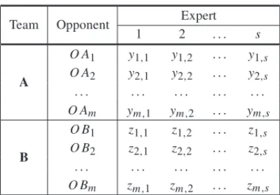
In order to formulate the prior distribution, a number of experts provide their expected final scores for the incoming matches which we intend to predict. This kind of elicitation procedure is natural and simple, since the model parameters are directly related to the number of goals and the requested information is readily understandable by the respondents not requiring any extra explanation. Differently from the usual empirical Bayes methods in which considers that the prior distribution is estimated from the data (Migon et al., 2014), we have adopted multiple experts since we believe it aggregates more information than using only one expert.
Assuming independent experts’ opinions and following a Poisson distribution, we shall obtain the prior distribution for the parameters using a procedure analogous to the power prior method (Chen & Ibrahim, 2000) with the historical data replaced by the experts’ expected scores. The proposed elicitation process is based on the assumption that the experts are able to provide plau-sible outcomes for the incoming matches that could be observed but in fact were not. This elic-itation process is in accordance with the bayesian paradigm for prior elicelic-itation as discussed in Genest & Zidek (1986) and Clemen & Winkler (1999) as we shall see later in this section. More-over, although the independence assumption is taken mainly because of mathematical simplicity, we can argue that, at least approximately, the independence assumption holds in our case since the selected experts work at different media and do not maintain any contact. They are sport experts on TV and newspapers specialised in sports.
Indeed, for predicting football match outcomes, various factors should be needed, such as changes in tactical patterns of teams, scoring or conceding a goal, injury or expulsion of an important player, presence of crisis in a team, performance of a team against other in former matches, among others. This type of data, although important, can be difficult to access. In particular thinking about teams that are competing in a WCT, where the amount of matches that were played between them may be very small. For instance, Brazil only once played against Ghana in 2006. It is at this juncture, data difficult access and small amount, that fits the use of information arising subjective priori experts. It fills the lack of information when there is short-age of objective information (data) available. In or case, we shall emphasize the importance of the experts information on the quality of the predictions in Section 4.1 (please see Fig. 2).
Table 1– Experts’ expected scores.
Team Opponent Expert
1 2 . . . s
A
O A1 y1,1 y1,2 . . . y1,s
O A2 y2,1 y2,2 . . . y2,s . . . .
O Am ym,1 ym,2 . . . ym,s
B
O B1 z1,1 z1,2 . . . z1,s
O B2 z2,1 z2,2 . . . z2,s . . . .
O Bm zm,1 zm,2 . . . zm,s
In the following, we shall assume as the initial information about the parameters the probability density function given by
π0(λA)∝λδA0−1exp{−β0λA}, (3)
and
π0(λB)∝λδB0−1exp{−β0λB}, (4)
whereδ0>0 andβ0≥0. Note that ifδ0=1/2 andβ0=0 we have the Jeffreys’ prior for the
Poisson model, ifδ0 =1 andβ0 =0 we have an uniform distribution over the interval(0,∞)
and ifδ0 >0 andβ0 > 0 we have a proper Gamma distribution. The first two cases are usual
choices to represent noninformative distribution for the parameter.
Updating this initial prior distribution with the experts’ expected scores, we obtain the power prior ofλA
π (λA|D0)∝λ a0
m
i=1 s
j=1
yi,j+δ0−1
A exp
−
a0s m
i=1 RA RO Ai
+β0
λA , (5)
where 0≤ a0 ≤ 1 represents a “weight” given to experts’ information andD0denotes all the
experts’ expected scores. Thus, if 0<a0≤1, the prior distribution ofλAis
λA|D0∼ Gamma
⎛
⎝a0 m
i=1 s
j=1
yi,j +δ0,a0s m
i=1 RA RO Ai
+β0
⎞
⎠,
The elicitation of the prior distribution(5) can also be viewed in the light of the bayesian paradigm of elicitation (Genest & Zidek, 1986), when we consider for the experts information the likelihood
L′(λA|y1,1, . . . ,ym,s)∝ m i=1 s j=1
λyAi,jexp
−λA RA RO Ai
a0
(6)
and combine it with the initial noninformative prior distribution (3) by applying the Bayes theo-rem. The likelihood (6) provides information for the parameter through the experts’ information, which are treated like data, i.e, we assume them to follow a Poisson distribution.
Analogously, the prior distribution ofλBis
π (λB|D0)∝λ a0
m
i=1 s
j=1
zi,j+δ0−1
B exp
−
a0s m
i=1 RB RO Bi
+β0
λB . (7)
It is important to note that by the way the experts present their opinions there is possibility of contradictory information. There is some literature on prior elicitation of group opinions directed towards to remove such inconsistencies. According to O’Hagan et al. (2006), they range from informal methods, such as Delphi method (Pill, 1971), which encourage the experts to discuss the issue in the hope of reaching consensus, to formal ones, such as weighted averages, opinion polling or logarithmic opinion pools. For a review of methods of pooling expert opinions see Genest & Zidek (1986).
2.2 Posterior and predictive distributions
Our interest is to predict the number of goals that team Ascored against teamB, using all the available information (hereafter denoted byD). This information is originated from two sources:
the experts’ expected score and the actual scores of matches already played. So, we may be in two distinct situations: (i) we do have the experts’ information but no matches have been played; (ii) we have both the experts’ opinions and the scores of played matches.
In situation (i), we only have the experts’ information. So, from the model (1) and the prior distribution (5), it follows that the prior predictive distribution ofXABis
XAB∼NB
⎛ ⎜ ⎜ ⎝ a0 m i=1 s j=1
yi,j +δ0, a0s
m
i=1 RA RO Ai +β0
a0s m
i=1 RA RO Ai +
RA RB +β0
⎞
⎟ ⎟ ⎠
, k=0,1, . . . , (8)
whereN B(r, γ )denotes the Negative Binomial distribution with probability function given by
f(k;r, γ )= Ŵ(r+k)
k!Ŵ(r) (1−γ )
kγr, k=
0,1, . . . ,
Analogously, from model (2) and the prior distribution (7), it follows that the prior predictive distribution ofXB Ais given by
XB A∼NB
⎛ ⎜ ⎜ ⎝ a0 m i=1 s j=1
zi,j +δ0, a0s
m
i=1 RB RO Bi +β0
a0s m
i=1 RB RO Bi +
RB RA +β0
⎞
⎟ ⎟ ⎠
, k=0,1, . . . . (9)
In situation (ii), assume that teamAhas playedkmatches, the first against teamC1, the second
against teamC2, and so on until the k-th match against team Ck. Suppose also that, givenλA, XA,C1, . . . ,XA,Ck are independent Poisson random variables with parameters
λA RA RC1
, . . . , λA RA RCk
.
Hence, from model (1) it follows that the likelihood is given by
L(λA|D)= k
i=1
PXA,Ci =x i A ∝exp −λA k i=1 RA RCi
λ
k
i=1 xiA
A , (10)
wherexiAare the number of goals scored byAagainst thei-th opponent,i=1, . . . ,k.
From the likelihood (10) and the prior distribution (5), it follows that the posterior distribution of λAis
λA|D∼ Gamma
⎛ ⎜ ⎜ ⎜ ⎜ ⎜ ⎝ a0 m i=1 s j=1 yi,j+
k
l=1
xlA+δ0,
k
l=1 RA RCl
+a0s m
i=1 RA RO Ai
+β0
⎞ ⎟ ⎟ ⎟ ⎟ ⎟ ⎠ , (11)
which implies by the model (1) that the posterior predictive distribution ofXABis
XAB|D∼ NB
⎛ ⎜ ⎜ ⎜ ⎜ ⎜ ⎜ ⎜ ⎜ ⎜ ⎝ a0 m i=1 s j=1 yi,j +
k
l=1
xlA+δ0,
k
l=1 RA RCl +a0s
m
i=1 RA RO Ai +β0 k
l=1 RA RCl +a0s
m
i=1 RA RO Ai +
RA RB +β0
⎞ ⎟ ⎟ ⎟ ⎟ ⎟ ⎟ ⎟ ⎟ ⎟ ⎠ . (12)
Analogously, the posterior distribution ofλB is given by
λB|D∼ Gamma
⎛ ⎜ ⎜ ⎜ ⎜ ⎜ ⎝ a0 m i=1 s j=1 zi,j +
k
l=1
xlB+δ0,
k
l=1 RB
RDl
+a0s m
i=1 RB
RO Bi
+β0
where xlB is the number of goals team B scores against thel-th opponent, Dl,l = 1, . . . ,k. Hence, from the model (2) and the posterior (13), it follows that the posterior predictive distribu-tion ofXB Ais
XB A|D∼ NB
⎛ ⎜ ⎜ ⎜ ⎜ ⎜ ⎜ ⎜ ⎜ ⎜ ⎝ a0 m i=1 s j=1 zi,j+
k
l=1
xlB+δ0,
k
l=1 RB RDl +a0s
m
i=1 RB RO Bi +β0 k
l=1 RB RDl +a0s
m
i=1 RB RO Bi +
RB RA +β0
⎞ ⎟ ⎟ ⎟ ⎟ ⎟ ⎟ ⎟ ⎟ ⎟ ⎠ . (14)
At this point, it is important to note that matches taken to construct the prior distribution are distinct from those considered to the likelihood function, that is, the matches already played have their contribution (through their final scores) included in the likelihood function but not in the prior.
3 METHODS
In this section, we shall consider the competition divided into 7 rounds, where the first three rounds are in the group stage (first phase) and the last four in the knockout stage (second phase). The 4 experts’ were asked for their expected final scores for the matches in 5 distinct times: just before the beginning of tournament and just before each of the 4 rounds in the knockout stage. At the beginning of competition, experts provided their expected final scores for all matches in the group stage at once, while in the knockout stage they provide their expected final scores only for matches in the incoming round. To account for the mean experts’ opinion, we have chosen
a0=1/(3∗4)=1/12 (for the group stage) anda0=1/4 (for the knockout stage), in the sense
that the posterior distribution of the parameter is the same as that, which would be obtained if we took one observation equal to the mean expected score from the sampling distribution. It is important to note that the experts were selected from different sports media, in order to make their guesses as independent as possible. In the Section 4 in the tournament prediction, we addressed the issue of thea0values choice.
In this paper, we have considered as the initial prior distribution (equations (3) and (4)) the Jeffreys’ prior, i.e.,δ0=1/2 andβ0 =0. We also have investigated other two possibilities for
noninformative distributions for the parameters: the uniform prior distribution over the interval (0,∞)(δ0 =1 andβ0 = 0), a vague Gamma prior (δ0 = 0.01 andβ0 = 0.01) and a vague
Exponential prior (δ0=1 andβ0=0.01).
of victory of teamAversus teamBequals the ratioa/(a+b)withaandbthe posterior means of the number of goals of teamsAandB, respectively.
The exact calculation of probabilities is possible just for the case of a single match prediction. We calculate the probabilities exactly from the predictive distributions. The probabilities regarding qualifying chances, winning tournament chances among others must be performed by simulation, since they may involves many combinations of match results.
3.1 Predictions for single matches
For a given match played by teams AandB, the probabilities of win (PW), draw (PD) and loss (PL) for teamAagainstBis obtained from the predictive distributions by using the expressions
PW =P(XAB>XB A)= ∞
i=1 i−1
j=0
P(XAB =i)P(XB A = j), (15)
PD =P(XAB=XB A)= ∞
i=0
P(XAB =i)P(XB A =i), (16)
and
PL = P(XAB<XB A)= ∞
j=1 j−1
i=0
P(XAB =i)P(XB A = j). (17)
It is useful to consider the set of all possible forecasts given by the simplex set
S=(PW,PD,PL)∈ [0,1]3: PW +PD+PL =1
.
Observe that the vertices(1,0,0), (0,1,0)and(0,0,1)ofS represent the outcomes win, draw and loss, respectively. Thus, a method used to measure the goodness of a prediction is to calculate the De Finetti distance (DeFinetti, 1972) which is the square of the Euclidean distance between the point corresponding to the outcome and the one corresponding to the prediction, e.g., if a prediction is(0.2,0.65,0.15)and the outcome is a draw(0,1,0), then the De Finetti distance is (0.2−0)2+(0.65−1)2+(0.15−0)2=0.185. Also, we can associate to a set of predictions the average of its De Finetti distances, known as the De Finetti measure. So, we shall consider the best among some prediction methods the one with the least De Finetti measure. Furthermore, the De Finetti value 2/3 can be considered as a reference for comparison, because an equiprobable predictor which assigns equal probability for all outcomes (PW =PD = PL =1/3) has 2/3 as its De Finetti measure.
For the matches of the first stage, the De Finetti measure for the Gamma, Uniform and Expo-nential priors were 43.90%, 50.18% and 44.70% higher than De Finetti measure for the Jeffreys’ prior, justifying our choice for the Jeffreys’ prior.
3.2 Predictions for the whole tournament
Besides the prediction of outcomes for a single match, we also use the predictive distributions to perform a simulation of 10.000 replicas of the whole competition. The purpose of this simulation is to estimate probabilities of events related to the competition as a whole such as the probability that a given team qualifies to the knockout stage, reaches the final, wins the tournament, and so on. The probabilities are estimated by the percentage of times the event of interest occurred and are presented in Section 4.
4 THE 2010 AND 2014 WCTS
The 2010 FIFA WCT took place in South Africa from 11 June to 11 July 2010. The following 32 teams were qualified for the tournament: Algeria, Argentina, Australia, Brazil, Cameroon, Chile, Denmark, England, France, Germany, Ghana, Greece, Honduras, Italy, Ivory Coast, Japan, Mexico, Netherlands, New Zealand, Nigeria, North Korea, Paraguay, Portugal, Serbia, Slovakia, Slovenia, South Africa, South Korea, Spain, United States, Uruguay, Switzerland. In the final, Spain defeated Netherlands 1-0 after extra time, to win the tournament.
The 2014 FIFA WCT took place in Brazil from 12 June to 13 July 2014. The following 32 teams were qualified for the tournament: Algeria, Argentina, Australia, Belgium, Bosnia & Herze-govina, Brazil, Cameroon, Chile, Colombia, Costa Rica, Croatia, Ecuador, England, France, Germany, Ghana, Greece, Honduras, Iran, Italy, Ivory Coast, Japan, Mexico, Holland, Nigeria, Portugal, Russia, South Korea, Spain, Switzerland, United States, Uruguay. In the final, Ger-many defeated Argentina 1–0 to win the tournament, securing the country’s fourth world title. Brazil lost to Germany in the semi-finals and finished the tournament in fourth place.
In this section apply the methodology present in the paper for both 2010 and 2014 FIFA WCTs. We present some of the results obtained by the application of our modelling for the cases of a single match prediction with and without previous observed data. We also illustrate the simula-tion methods performed to obtain the probabilities of qualifying to the knockout stage, reaching quarter finals, semi finals, the final match and being the champion.
4.1 2010 WCT – Single Match Prediction
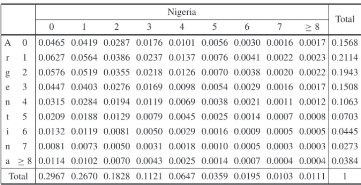
We illustrate the predictions for the match Argentina versus Nigeria in Group B which occurred in the first round. The mean experts’ expected final score for this match was 2−0.75 for Argentina against Nigeria. We observe a very large difference in skill between the two teams expressed by their different FIFA ranking positions, 7-th and 18-th (please see Table 10 in appendix). Table 2 presents the calculated score probabilities for this match. The observed result was 1-0 for Ar-gentina, which is one of the most plausible results according to Table 2 (6.27%). The winning probabilities for Argentina is 55.47%, for Nigeria is 17.62% and a draw has probability 26.91%.
Table 2– Score chances for the match Argentina versus Nigeria.
Nigeria
Total
0 1 2 3 4 5 6 7 ≥8
A 0 0.0465 0.0419 0.0287 0.0176 0.0101 0.0056 0.0030 0.0016 0.0017 0.1568
r 1 0.0627 0.0564 0.0386 0.0237 0.0137 0.0076 0.0041 0.0022 0.0023 0.2114
g 2 0.0576 0.0519 0.0355 0.0218 0.0126 0.0070 0.0038 0.0020 0.0022 0.1943 e 3 0.0447 0.0403 0.0276 0.0169 0.0098 0.0054 0.0029 0.0016 0.0017 0.1508
n 4 0.0315 0.0284 0.0194 0.0119 0.0069 0.0038 0.0021 0.0011 0.0012 0.1063
t 5 0.0209 0.0188 0.0129 0.0079 0.0045 0.0025 0.0014 0.0007 0.0008 0.0703
i 6 0.0132 0.0119 0.0081 0.0050 0.0029 0.0016 0.0009 0.0005 0.0005 0.0445
n 7 0.0081 0.0073 0.0050 0.0031 0.0018 0.0010 0.0005 0.0003 0.0003 0.0273 a ≥8 0.0114 0.0102 0.0070 0.0043 0.0025 0.0014 0.0007 0.0004 0.0004 0.0384
Total 0.2967 0.2670 0.1828 0.1121 0.0647 0.0359 0.0195 0.0103 0.0111 1
are 0.4423, 0.4445 and 0.53, while the proportion of correct prediction are 66.67%, 75% and 50%, respectively. All the outcome predictions change slightly with the incorporation of ob-served data, except from the prediction for the match Portugal versus Korea DPR in the second round. Portugal win probability has decreased from 77.5% to 55% and the Korea win raise from 11.3% to 23.8% with the observation of outcomes of the first round.
Table 3– Predictions for the matches of Group G.
Round Team Observed Team W D L De Correct
score Finetti
1 Cˆote d’Ivoire (0-0) Portugal 0.340 0.159 0.501 1.074 N
1 Brazil (2-1) Korea DPR 0.775 0.127 0.099 0.076 Y
Before 2 Brazil (3-1) Cˆote d’Ivoire 0.527 0.175 0.298 0.343 Y
1st round 2 Portugal (7-0) Korea DPR 0.771 0.116 0.113 0.079 Y
3 Portugal (0-0) Brazil 0.362 0.198 0.439 0.967 N
3 Korea DPR (0-3) Cˆote d’Ivoire 0.153 0.123 0.723 0.115 Y 2 Brazil (3-1) Cˆote d’Ivoire 0.556 0.227 0.217 0.296 Y
Before 2 Portugal (7-0) Korea DPR 0.550 0.212 0.238 0.304 Y
2nd round 3 Portugal (0-0) Brazil 0.247 0.268 0.485 0.832 N
3 Korea DPR (0-3) Cˆote d’Ivoire 0.282 0.196 0.522 0.346 Y
Before 3 Portugal (0-0) Brazil 0.300 0.230 0.470 0.903 N
3rd round 3 Korea DPR (0-3) Cˆote d’Ivoire 0.152 0.171 0.677 0.157 Y
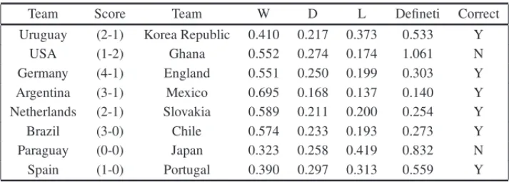
Table 4 shows the probabilities attached to the outcomes (results in 90 minutes, in other words, in regulation time), the De Finetti measures and correct prediction indicator for matches of Round of 16 phase. The DeFineti measure for this round is 0.4944 and the correct prediction proportion 75%.
Table 4– Predictions for the round of 16.
Team Score Team W D L Defineti Correct
Uruguay (2-1) Korea Republic 0.410 0.217 0.373 0.533 Y
USA (1-2) Ghana 0.552 0.274 0.174 1.061 N
Germany (4-1) England 0.551 0.250 0.199 0.303 Y
Argentina (3-1) Mexico 0.695 0.168 0.137 0.140 Y
Netherlands (2-1) Slovakia 0.589 0.211 0.200 0.254 Y
Brazil (3-0) Chile 0.574 0.233 0.193 0.273 Y
Paraguay (0-0) Japan 0.323 0.258 0.419 0.832 N
Spain (1-0) Portugal 0.390 0.297 0.313 0.559 Y
For the final matches (first and third place matches), the chances for each finalist are presented in Table 5. Despite the optimism of experts in favor of Spain (mean expected score 1.25−0.75) and the best FIFA ranking (2nd against 4th), the lower number of goals scored in the tournament in comparison with Netherlands (7 versus 12) resulted in a slight favoritism to the Netherlands (56.79% Netherlands victory against 43.21% for Spain victory).
For the third place match, Germany versus Uruguay, we observe a widespread predicted fa-voritism of Germany (72.32% Germany win against 27.68% Uruguay win), which can be ex-plained by its best performance in previous matches (13 goals scored against 9), its highest ranking position (6th against 13th) and the significant wins against strong and traditional teams such as England (Germany 4-1 England) and Argentina (Germany 4-0 Argentina), which also affected the experts’ opinions in favor of Germany (the mean expected score was 1.75 against 1.25).
Table 5– Prediction for the final and third place match.
Team Champion 2nd Place 3rd Place 4th Place
Spain 0.4321 0.5679 0.0000 0.0000
Netherlands 0.5679 0.4321 0.0000 0.0000
Germany 0.0000 0.0000 0.7232 0.2768
Uruguay 0.0000 0.0000 0.2768 0.7232
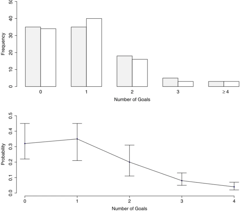
procedure, following Bittner et al. (2009) and Janke et al. (2009), we plot in the lower panel of Figure 1 the relative observed frequency of the number of goals, superimposed by the lower and upper quantiles (0.025 and 0.975) of the predictive density over 1,000 replications of the whole tournament. There is no important deviations, indicating the data fit well the assumed model.
For sake of comparison we also considered a model where a discrete uniform distribution in the interval 0 to 4 is assumed for the number of goals of any team in any match in the competition, thea0is assumed to be equal to 0 and the FIFA rank is assumed to be equal to all teams. Such
model can be regarded as a sort of random guessing model. In this case, the usual chi-square test for adherence comparing the observed and expected number of goals produced a p-value smaller than 0.00001, indicating that the deviations of the random guessing model from the truth are substantially bigger than what would be expected if it is the true model.
0 1 2 3 ≥4
Number of Goals
Frequency
0
1
02
03
04
05
0
●
●
●
●
●
0 1 2 3 4
0.0
0.1
0.2
0.3
0.4
0.5
Number of Goals
Probability
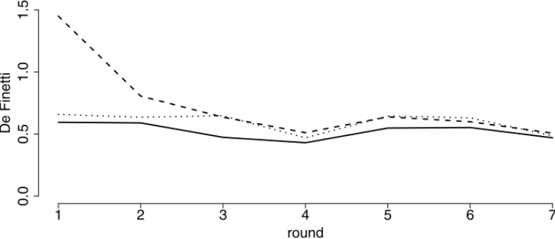
In order to assess the impact of the experts’ information on the quality of the predictions, Figure 2 displays the DeFinetti measure for our pool of experts fixinga0at 0 and 0.25, denoting
respec-tively the total absence of experts’ opinion and the amount of experts’ information as considered to account for the mean of their opinion in our method. Moreover, for sake of comparison with the best possibility, we replaced our experts’ information by a fictitious pool of “perfect” experts, who always forecast the exact score for each one of the matches, witha0fixed 0.25.
At the initial rounds, the use of experts’ information greatly improves prediction, with the De-Finetti measure witha0 = 0.25 always closer to the results of the “perfect” experts’ opinion.
However, as observed data enters the model, with the progress of the competition, the gain of using expert information is decreasing. This feature is in fully agreement with our initial motiva-tion to consider experts’ informamotiva-tion in our modeling: filling the lack of informamotiva-tion when there is shortage of objective information (data) available. For the knockout stage matches, experts’ information did not improve prediction, which can be explained in part by the small difference of skill level between teams and by the lack of confidence on Spain and Netherlands teams who defeated the traditional teams of Germany and Brazil, respectively.
1 2 3 4 5 6 7
0.0
0.5
1.0
1.5
round
De Finetti
Figure 2– De Finetti measure considering our pool of experts witha0 =0 (dashed line) anda0= 0.25 (dotted line). The solid line represents the case of a fictitious pool of “perfect” experts witha0=0.25.
4.2 2010 WCT – Classification Predictions at Group Stage
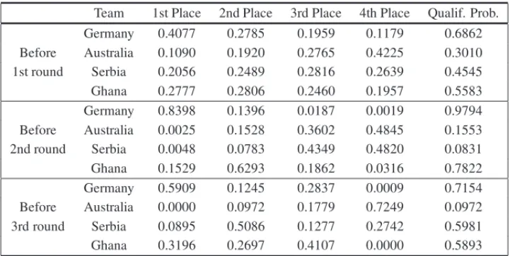
In this section, we illustrate how the simulation procedure is applied to calculate the qualifying probabilities for Group D, compose by the teams: Autralia, Germany, Ghana and Serbia.
After 1st round, we can see that the Germany team confirmed the favoritism and thrashed Aus-tralia (4-0), increasing its qualifying chance and more than doubling the chance of finishing in the first place. At the 1st round, Serbia was defeated by Ghana and its qualifying chances has decreased from 45.45% to 8.31%. On the other hand, Ghana increased its qualifying chances from 55.83% to 78.22%.
Table 6– Classification forecasts for group D.
Team 1st Place 2nd Place 3rd Place 4th Place Qualif. Prob.
Germany 0.4077 0.2785 0.1959 0.1179 0.6862
Before Australia 0.1090 0.1920 0.2765 0.4225 0.3010
1st round Serbia 0.2056 0.2489 0.2816 0.2639 0.4545
Ghana 0.2777 0.2806 0.2460 0.1957 0.5583
Germany 0.8398 0.1396 0.0187 0.0019 0.9794
Before Australia 0.0025 0.1528 0.3602 0.4845 0.1553
2nd round Serbia 0.0048 0.0783 0.4349 0.4820 0.0831
Ghana 0.1529 0.6293 0.1862 0.0316 0.7822
Germany 0.5909 0.1245 0.2837 0.0009 0.7154
Before Australia 0.0000 0.0972 0.1779 0.7249 0.0972
3rd round Serbia 0.0895 0.5086 0.1277 0.2742 0.5981
Ghana 0.3196 0.2697 0.4107 0.0000 0.5893
After the second round, the “unexpected” (1-0) Serbia win against Germany, increased consid-erably Serbia’s qualifying chances (from 8.31% to 59.81%) and decreased Germany’s chances from 97.94% to 71.54%. The great increase in Serbia’s qualifying chances can be explained by the fact that, besides of winning three points, Serbia beat the very strong German team and will play at the final round against the weak Australia team. The (1-1) draw in the match Australia versus Ghana let all teams with chances of qualifying for the next stage, with Serbia and Ghana having very similar qualifying chances.
After the third round, Germany confirmed the predictions and defeated Ghana (1-0). On the other hand, Serbia lost its match against Australia and finished in the fourth place. Despite its defeat, Ghana classified in the second place.
4.3 2010 WCT – Tournament Prediction
In this section, we present the results of the simulation study performed to estimate probabilities of events related to the tournament. A quantity of 10,000 tournament replicas has been carried out in each simulation.
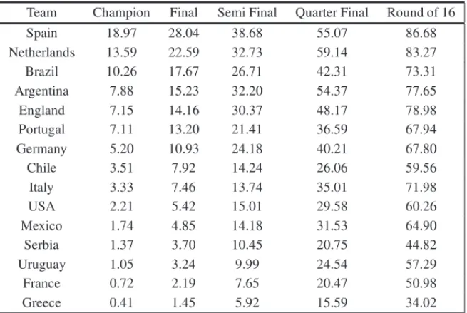
also an equilibrium among Argentina, England and Portugal. Surprisingly, the traditional teams of France and Italy (who joined the 2006 WCT final match) have less chances than Chile and Portugal. Actually, France and Italy did not qualified for the knockout stage.
Table 7– Probabilities of the 16 top teams for the next phases.
Team Champion Final Semi Final Quarter Final Round of 16
Spain 18.97 28.04 38.68 55.07 86.68
Netherlands 13.59 22.59 32.73 59.14 83.27
Brazil 10.26 17.67 26.71 42.31 73.31
Argentina 7.88 15.23 32.20 54.37 77.65
England 7.15 14.16 30.37 48.17 78.98
Portugal 7.11 13.20 21.41 36.59 67.94
Germany 5.20 10.93 24.18 40.21 67.80
Chile 3.51 7.92 14.24 26.06 59.56
Italy 3.33 7.46 13.74 35.01 71.98
USA 2.21 5.42 15.01 29.58 60.26
Mexico 1.74 4.85 14.18 31.53 64.90
Serbia 1.37 3.70 10.45 20.75 44.82
Uruguay 1.05 3.24 9.99 24.54 57.29
France 0.72 2.19 7.65 20.47 50.98
Greece 0.41 1.45 5.92 15.59 34.02
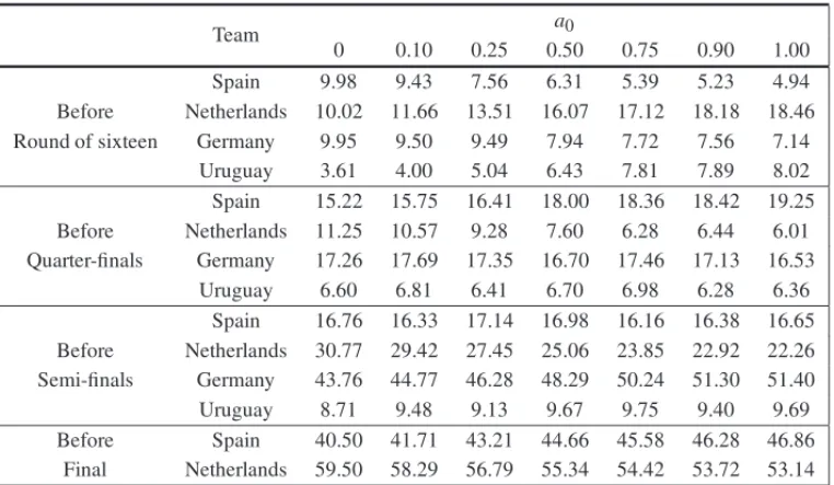
Considering only the four finalists (Spain, Netherlands, Germany and Uruguay) we obtained, just before each round of the knockout stage, the winning tournament probabilities assuming different values for thea0weight attached to the experts’ information. Table 9 presents the obtained results
for this simulation study. In all situations, varying thea0value we obtain different predictions
for the probability of tournament win for the teams, which means that predictions are sensible to different degrees of confidence on experts’ information.
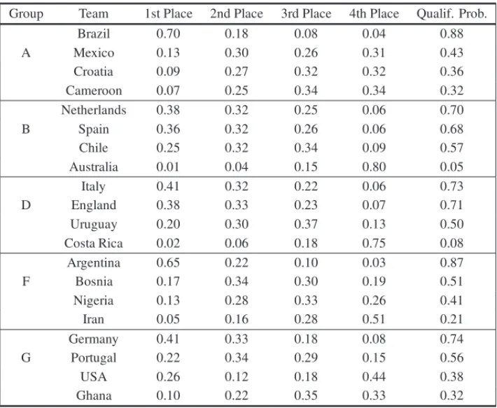
4.4 2014 WCT – Group Stage Classification Probalities
From now on we focus on the 2014 WCT. In this section, we illustrate how the simulation procedure is applied to calculate the qualifying probabilities for Groups A (Brazil Group), B (Spain Group, the champion of the 2010 WCT), D (Group of Death with the 3 ex-champions: Italy, England and Uruguay), F (Argentina Group, in the actual 2nd place) and G (German Group, actual champion).
Table 8– Classification forecasts for Groups A, B, D, F and G of the 2014 WCT.
Group Team 1st Place 2nd Place 3rd Place 4th Place Qualif. Prob.
Brazil 0.70 0.18 0.08 0.04 0.88
A Mexico 0.13 0.30 0.26 0.31 0.43
Croatia 0.09 0.27 0.32 0.32 0.36
Cameroon 0.07 0.25 0.34 0.34 0.32
Netherlands 0.38 0.32 0.25 0.06 0.70
B Spain 0.36 0.32 0.26 0.06 0.68
Chile 0.25 0.32 0.34 0.09 0.57
Australia 0.01 0.04 0.15 0.80 0.05
Italy 0.41 0.32 0.22 0.06 0.73
D England 0.38 0.33 0.23 0.07 0.71
Uruguay 0.20 0.30 0.37 0.13 0.50
Costa Rica 0.02 0.06 0.18 0.75 0.08
Argentina 0.65 0.22 0.10 0.03 0.87
F Bosnia 0.17 0.34 0.30 0.19 0.51
Nigeria 0.13 0.28 0.33 0.26 0.41
Iran 0.05 0.16 0.28 0.51 0.21
Germany 0.41 0.33 0.18 0.08 0.74
G Portugal 0.22 0.34 0.29 0.15 0.56
USA 0.26 0.12 0.18 0.44 0.38
Ghana 0.10 0.22 0.35 0.33 0.32
4.5 2014 WCT – Tournament Prediction
In this section, we present the results of the simulation study performed to estimate probabilities of events related to the 2014 tournament. A quantity of 10,000 tournament replicas has been carried out in each simulation.
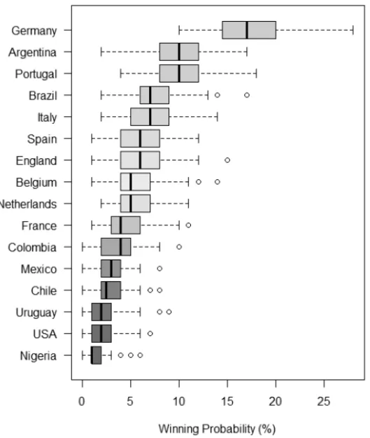
Before the beginning of tournament, a simulation was performed to calculate the chances of win-ning the championship. Figure 3 displays the Box-plot for the chances of winwin-ning the 2010 WCT for the top 16 teams. Based on this results, we observe a large favouritism of Germany, following by an equilibrium between Argentina and Portugal and sequencially Brazil. Netherlands appears more ahead but still with a good chance. Indeed, the four finalists were Germany, Argentina, Netherlands and Brazil.
5 FINAL REMARKS
Figure 3– Box-plot for the chances of winning the 2014 WCT before the tournament starts.
further and compared with the FIFA ratings. Moreover, the development of two ratings for teams, possibly via experts’ information or even FIFA documentation, one for attack and another for defense, could improve prediction since there are teams which have strong defense but weak attack and vice-versa. A simple possibility to incorporate those abilities would be to add one parameter for each team directly on the Poisson model, as it was made for instance in Volf (2009). This major embedding can be seen as a direct generalization of our modeling and should be considered in future research in the field.
The prior distributions are updated every round, providing flexibility to the modeling, once the experts’ opinion are influenced by all previous events to the match. The use of expert’s opinions may compensate, at least in part, for the lack of information of the factors which can influence a football match during a competition, such as tactic disciplines, team psychological conditions, referee, player injured or suspended, amongst others.
Moreover, the method presents a high performance within a simulation structure since known predictive distributions are obtained. This enables a rapid generation of predictive distribution values and consequently the probabilities of interest are obtained quickly.
For sake of comparison of our approach with other methodologies applied for predicting match outcomes of WCTs, we consider the methodology proposed by Bastos & da Rosa (2013). While the overall DeFinetti measure for their best predictive model for the 2010 WCT are 0.626 and 0.611, respectively for group stage and overall, our modeling performance is better with 0.568 and 0.570, respectively for the group stage and overall. Besides, our modeling joined a predic-tion model competipredic-tion for the matches of the group stage of the 2010 WCT organized by the Brazilian Society of Operational Research, the World Cup 2010 Football Forecast Competition, reaching the first place. We believe the inclusion of subjective information into our modeling through expert’s opinions was crucial for such achievements.
For the 2010 WCT, the forecasts presented in this paper as well as others results were avail-able and updated before each round on the website www.copa2010.ufscar.br. The internet users could also provide their guess on the match scores, interacting with our model through a chances simulator. The simulator uses an unique and innovative technology which makes an interac-tion between the programming languages such as PHP, HTML, CSS, JavaScript, SQL and R, to provide real time answers. In this context, the internet users were provided with all the teams’ chances of winning in each stage of the knockout stage as well as the chance of each team to be the champion. At that time, according to our counter, we had over 53,000 site visits with over 11,000 simulations made. Thus, a large number of internet users and viewers had been exposed to our methodology.
For the 2014 WCT, the forecasts presented in this paper as well as others results were available and updated before each round on the website www.previsaoesportiva.com.br/ copa. At that time, according to our counter, we had almost 50,000 site visits.
In our analysis the weights of the experts’ opinion are fixed and known. As further work it may be considered one distinct value ofa0for each expert and round allowing changes of the values over the rounds. One interpretation that can be made is that, for a particular expert, ifa0increases over
the rounds, the confidence of the information given by this expert increases as well. Alternatively, ifa0decreases, that means the information provided by this expert in previous rounds were not
reliable. Furthermore, we can assume thata0 is a random variable and use a full hierarchical
structure specifying a parametric distribution for the parameter a0, like a beta distribution, as suggested in Chen & Ibrahim (2000).
we considered here noninformative Jeffreys’ prior distributions for the Poisson parameters λA andλB. However, other prior distributions could be work well such as a bounded gamma one. Moreover, here the predictive distributions were computed separately, since our model and prior distribution are factorable in terms of function ofλAandλB. However, another approach would be the consideration of bivariate models as discussed in Karlis & Ntzoufras (2009), which allows for dependence between the number of goals of teams.
In our modeling we assume the presence of independence between the expert’s opinions, which simplifies the obtained mathematical expressions. However, a more realistic approach would assume an exchangeable distribution or a multivariate distribution with dependence structure modeled via copulas or other means. Future developments of the model should also consider such model enlargement.
Table 9– Percentage of tournament wins.
Team a0
0 0.10 0.25 0.50 0.75 0.90 1.00
Spain 9.98 9.43 7.56 6.31 5.39 5.23 4.94
Before Netherlands 10.02 11.66 13.51 16.07 17.12 18.18 18.46 Round of sixteen Germany 9.95 9.50 9.49 7.94 7.72 7.56 7.14
Uruguay 3.61 4.00 5.04 6.43 7.81 7.89 8.02
Spain 15.22 15.75 16.41 18.00 18.36 18.42 19.25 Before Netherlands 11.25 10.57 9.28 7.60 6.28 6.44 6.01 Quarter-finals Germany 17.26 17.69 17.35 16.70 17.46 17.13 16.53
Uruguay 6.60 6.81 6.41 6.70 6.98 6.28 6.36
Spain 16.76 16.33 17.14 16.98 16.16 16.38 16.65 Before Netherlands 30.77 29.42 27.45 25.06 23.85 22.92 22.26 Semi-finals Germany 43.76 44.77 46.28 48.29 50.24 51.30 51.40
Uruguay 8.71 9.48 9.13 9.67 9.75 9.40 9.69
Before Spain 40.50 41.71 43.21 44.66 45.58 46.28 46.86
Final Netherlands 59.50 58.29 56.79 55.34 54.42 53.72 53.14
That is, the changes in the result of Spain and Paraguay match leads to changes, but does not drastic, in the final results, yet pointing to a balanced match. Indeed, the last match was very hard to Spain, which scored a goal only in the extra time. There is now a number of methods on how to predict the outcomes of football matches or even matches of other kind of sport, some of then cited in the references. A large sample comparison of their accuracy could be an important future research theme in the light of our modeling.
Finally, at least in principle, the proposed methodology can be used for prediction of match out-comes of other sports, for instance, indoor soccer, basketball, water polo, handball and hockey, but taking into account the differences of tournament structure of each one.
ACKNOWLEDGMENTS
The authors thanks the Editorial Boarding and the anonymous referees for their criticisms, com-ments and suggestions on an early version of the manuscript. The research is partially supported by CNPq, CAPES and FAPESP.
REFERENCES
[1] ALVES AM, DE MELLO JCCBS, RAMOSTG & SANT’ANNAAP. 2011. Logit models for the probability of winning football games.Pesquisa Operacional,31(3): 459–465.
[2] BAIO G & BLANGIARDO M. 2010. Bayesian hierarchical model for the prediction of football results.Journal of Applied Statistics,37(2): 253–264.
[3] BASTOSLS & DAROSAJMC. 2013. Predicting probabilities for the 2010 fifa world cup games using a poisson-gamma model.Journal of Applied Statistics,40(7): 1553–1544.
[4] BITTNERE, NUSSBAUMERA, JANKEW & WEIGELM. 2009. Football fever: Goal distributions and non-gaussian statistics.European Physical Journal B,67(3): 459–471.
[5] CALOBAˆ GM & LINSMPE. 2006. Performance assessment of the soccer teams in brazil using dea.
Pesquisa Operacional,26(3): 521–536.
[6] CLEMENRT & WINKLERRL. 1999. Combining probability distributions from experts in risk anal-ysis.Risk Analysis,19(2): 187–103.
[7] DOBSONS & GODDARDJ. 2003. Persistence in sequences of football match results: A monte carlo analysis.European Journal of Operational Research,148(2): 247–256.
[8] GENEST C & ZIDEKJV. 1986. Combining probability distributions: a critique and an annotated bibliography.Statistical Science,1(1): 114–148.
[9] JANKE W, BITTNER E, NUSSBAUMERA & WEIGEL M. 2009. Football fever: self-affirmation model for goal distributions.Condensed Matter Physics,12(4): 739–752.
[10] KARLISD & NTZOUFRASI. 2009. Bayesian modelling of football outcomes: Using the Skellam’s distribution for the goal difference.IMA J. Manag. Math.,20: 133–145.
[12] KOOPMANSJ & LIT R. 2015. A dynamic bivariate poisson model for analysing and forecasting match results in the english premier league.Journal of the Royal Statistical Society Series A,178(1): 167–186.
[13] LOUZADA F, SUZUKIAK & SALASARLEB. 2014. Predicting match outcomes in the english premier league: Which will be the final rank?Journal of Data Science,12: 235–254.
[14] O’HAGAN A, BUCK CE, DANESHKHAH A, EISER JR, GARTHWAITE PH, JENKINSON DJ, OAKLEYJE & RAKOWT. 2006.Uncertain judgements: eliciting experts’ probabilities. John Wiley, London.
[15] SANT’ANNAAP. 2008. Rough sets analysis with antisymmetric and intransitive attributes: Classifi-cation of brazilian soccer clubs.Pesquisa Operacional,28(2): 217–230.
[16] SCARFFPA & SHIX. 2008. The importance of a match in a tournament.Computers & Operations Research,35(7): 2406–2418.
[17] SUZUKIAK, SALASARLEB, LOUZADA-NETOF & LEITE JG. 2009. A bayesian approach for predicting match outcomes: The 2006 (association) football world cup.Journal of the Operational Research Society,61: 1530–1539 (October 2010).
[18] VOLFP. 2009. A random point process model for the score in sport matches.IMA J. Manag. Math., 20: 121–131.
APPENDICE A: FIFA RATINGS
Table 10– FIFA ratings prior to 2010 WCT.
Team Group FIFA ratings Team Group FIFA ratings
Brazil G 1611 Australia D 886
Spain H 1565 Nigeria B 883
Portugal G 1249 Switzerland H 866
Netherlands E 1231 Slovenia C 860
Italy F 1184 Cˆote d’Ivoire G 856
Germany D 1082 Algeria C 821
Argentina B 1076 Paraguay F 820
England C 1068 Ghana D 800
France A 1044 Slovakia F 777
Greece B 964 Denmark E 767
USA C 957 Honduras H 734
Serbia D 947 Japan E 682
Uruguay A 899 Korea Republic B 632
Mexico A 895 New Zealand F 410
Chile H 888 South Africa A 392