www.biogeosciences.net/8/2009/2011/ doi:10.5194/bg-8-2009-2011
© Author(s) 2011. CC Attribution 3.0 License.
Biogeosciences
Controls on winter ecosystem respiration in temperate
and boreal ecosystems
T. Wang1, P. Ciais1, S. L. Piao2, C. Ottl´e1, P. Brender1, F. Maignan1, A. Arain3, A. Cescatti4, D. Gianelle5, C. Gough6, L. Gu7, P. Lafleur8, T. Laurila9, B. Marcolla10, H. Margolis11, L. Montagnani12,13, E. Moors14, N. Saigusa15,
T. Vesala16, G. Wohlfahrt17, C. Koven18, A. Black19, E. Dellwik20, A. Don21, D. Hollinger22, A. Knohl23, R. Monson24, J. Munger25, A. Suyker26, A. Varlagin27, and S. Verma26
1LSCE/IPSL, UMR8212, CEA-CNRS-UVSQ – Unit´e Mixte de Recherche, CE L’Orme des Merisiers, Gif-sur-Yvette 91191, France
2Department of Ecology, College of Urban and Environmental Science, and Key Laboratory for Earth Surface Processes of the Ministry of Education, Peking University, Beijing 100871, China
3School of Geography and Earth Sciences, McMaster University, Hamilton, ON, L8S 4K1, Canada
4Climate Change Unit, Inst. for Environment and Sustainability, European Commission, DG joint Research Centre, Ispra, Italy
5IASMA, Research and Innovation Centre, Fondazione Edmund Mach, Viote del Monte Bondone, Trento, 38040, Italy 6Deparment of Biology, Virginia Commonwealth University, P.O. Box 842012, 1000 West Cary St. Richmond, VA 23284-2012, USA
7Environmental Sciences Division, Oak Ridge National Laboratory, Oak Ridge, TN 37831, USA 8Department of Geography, Trent University, Peterborough, Ontario K9J 7B8, Canada
9Finnish Meteorological Institute, P.O. Box 503, 00101 Helsinki, Finland
10Edmund Mach Foundation, Research and Innovation Center, 38010 S. Michele all’ Adige, Trento, Italy 11Centre d’ ´Etude de la Foret, Facult´e de Foresterie, de G´eographie et de G´eomatique, Universit´e Laval, Qu´ebec, QC, G1V 0A6, Canada
12Autonomous Province of Bolzano, Forest Services and Agency for the Environment, Bolzano, Italy 13Free University of Bolzano, Faculty of Science and Technology, Bolzano, Italy
14Alterra Wageningen UR, Wageningen, 6700 AA, The Netherlands
15Center for Global Environmental Research, National Institute for Environmental Studies, 16-2 Onogawa, Tsukuba 305-8506, Japan
16Department of Physics, University of Helsinki, P.O. Box 48, 00014, Finland
17University of Innsbruck, Institute of Ecology Sternwartestrasse 15, Innsbruck 6020, Austria 18Lawrence Berkeley National Lab, Berkeley 94720, CA, USA
19Faculty of Land and Food systems, University of British Columbia, Vancouver, British Columbia, V6T 1Z4, Canada 20Wind Energy Division, Risoe National Laboratory for Sustainable Energy, Technical University of Denmark, P.O. Box 49, 4000 Roskilde, Denmark
21Johann Heinrich von Th¨unen Inst., Inst. of Agricultural Climate Research, Bundesallee 50, 38116 Braunschweig, Germany 22Northern Research Station, USDA Forest Service, 271 Mast Rd, Durham, NH 03824, USA
23Chair of Bioclimatology, B¨usgen Institute, Georg-August University of G¨ottingen, Germany
24Department of Ecology and Evolutionary Biology, University of Colorado, Boulder, CO 80309, USA
25Division of Engineering and Applied Science, Deptment of Earth and Planetary Science, Harvard University, Cambridge, MA 02138, USA
26School of Natural Resources, University of Nebraska-Lincoln, Lincoln, NE 68583, USA
27A. N. Severtsov Institute of Ecology and Evolution, Russia Academy of Sciences, Leninsky Prospect 33, Moscow, 117071, Russia
Received: 5 August 2010 – Published in Biogeosciences Discuss.: 15 September 2010 Revised: 20 June 2011 – Accepted: 29 June 2011 – Published: 25 July 2011
Abstract. Winter CO2 fluxes represent an important com-ponent of the annual carbon budget in northern ecosys-tems. Understanding winter respiration processes and their responses to climate change is also central to our abil-ity to assess terrestrial carbon cycle and climate feedbacks in the future. However, the factors influencing the spa-tial and temporal patterns of winter ecosystem respiration (Reco) of northern ecosystems are poorly understood. For this reason, we analyzed eddy covariance flux data from 57 ecosystem sites ranging from ∼35◦N to ∼70◦N. Decidu-ous forests were characterized by the highest winter Reco rates (0.90±0.39 g C m−2d−1), when winter is defined as the period during which daily air temperature remains below 0◦C. By contrast, arctic wetlands had the lowest winterR
eco rates (0.02±0.02 g C m−2d−1). Mixed forests, evergreen needle-leaved forests, grasslands, croplands and boreal wet-lands were characterized by intermediate winter Reco rates (g C m−2d−1) of 0.70(±0.33), 0.60(±0.38), 0.62(±0.43), 0.49(±0.22) and 0.27(±0.08), respectively. Our cross site analysis showed that winter air (Tair) and soil (Tsoil) temper-ature played a dominating role in determining the spatial pat-terns of winterRecoin both forest and managed ecosystems (grasslands and croplands). Besides temperature, the sea-sonal amplitude of the leaf area index (LAI), inferred from satellite observation, or growing season gross primary pro-ductivity, which we use here as a proxy for the amount of recent carbon available for Reco in the subsequent winter, played a marginal role in winter CO2emissions from forest ecosystems. We found that winterReco sensitivity to tem-perature variation across space (QS) was higher than the one
over time (interannual,QT). This can be expected because
QS not only accounts for climate gradients across sites but
also for (positively correlated) the spatial variability of sub-strate quantity. Thus, if the models estimate future warming impacts onRecobased onQSrather thanQT, this could
over-estimate the impact of temperature changes.
1 Introduction
The processes controlling the winter carbon cycle of northern ecosystems, which is mainly ecosystem respiration (Reco), have received much less attention than processes active dur-ing the growdur-ing season. The longstanddur-ing view of marginal wintertime biological activity (e.g. Coyne and Kelley, 1971; Steudler et al., 1989) proposes that winter respiration is very small compared to growing season respiration. Recent field studies suggest a different picture by demonstrating the larger than expected wintertime respiration rates in Arctic tundra, bog, and mountain ecosystems (e.g. Oechel et al., 1997; Fahnestock et al., 1998; Grogan and Chapin, 1999; Panikov and Dedysh, 2000; Aurela et al., 2002; Monson et al., 2006; Bergeron et al., 2007). These studies suggest that winterReco should not be ignored when attempting to
quantify and understand the annual carbon balance of terres-trial ecosystems (Hobbie et al., 2000; Grogan and Jonasson, 2005; Johansson et al., 2006). However, due to the large car-bon storage and heterogeneity of northern ecosystems, win-terRecoremains incompletely understood given the limited spatial representativeness of individual-site studies.
In general, mid and high-latitude ecosystems contain large amounts of soil carbon (Post et al., 1982; Tarnocai et al., 2009), which implies that these ecosystems could provide a significant positive feedback to climate change if warming stimulates soil carbon decomposition and CO2release to the atmosphere (Friedlingstein et al., 2006). The increased high-latitude warming projected by climate models includes win-ter warming (Serreze et al., 2000; Giorgi et al., 2001) and has already been observed over the past 30 yr (IPCC, 2007). The response of the soil organic carbon (SOC) balance to warming differs widely among coupled climate-carbon mod-els (Friedlingstein et al., 2006). This is because the net bal-ance in these models depends on two fluxes of opposite di-rections: the litter input that may increase under warming if vegetation net primary productivity increases, and the soil carbon microbial decomposition rate that also responds posi-tively to warming (e.g. Jones et al., 2005). Therefore, it is im-portant to disentangle how temperature and vegetation pro-ductivity separately affect winter respiration. Previous stud-ies (e.g. Clein and Schimel, 1995; Hobbie, 1996; Mikan et al., 2002; Grogan et al., 2001; Grogan and Jonasson, 2005) were concentrated on the site-level or landscape-level. For example, Grogan and Jonasson (2005) found that both the amount of substrate available for respiration and soil tem-perature (Tsoil)determine landscape-level variation of winter Recoof birch forest and heath tundra. These studies are valu-able for understanding site-specific or landscape-level pro-cesses, but their results cannot be readily extrapolated across sites and climate gradients to infer regional sensitivities.
the latter not only accounts for direct climate effects, but also site productivity (Mahecha et al., 2010; Wang et al., 2010). Finally, in an attempt to improve our understanding of spa-tial controls on winterReco, we examine the relationships be-tween winterReco, climate variables and productivity-related variables across sites.
2 Materials and methods
2.1 Data sources
2.1.1 Eddy covariance flux data
The eddy covariance data used in this study are extracted from the La Thuile FLUXNET synthesis database which contains 965 site years processed according to standardized protocols (Papale et al., 2006) (http://www.fluxdata.org). The processing of this dataset is based on friction veloc-ity (u∗) filter and despiking of half hourly flux data, which would be expected to reduce the bias of flux measurements during the calm night and winter stable stratification period. Daily cumulative values of Net Ecosystem Exchange (NEE, g C m−2day−1)are retrieved from the half hourly values in-cluded in the database, where a positive NEE represents a carbon release and a negative NEE a carbon uptake. The NEE time series can be partitioned into gross primary pro-ductivity (GPP) and ecosystem respiration (Reco). The flux-partitioning algorithm, which is implemented in La Thuile FLUXNET database, uses short-term temperature sensitiv-ities to extrapolate night-time respiration to daytime. This approach avoids significantly biased estimates ofReco that can be obtained using long-term temperature sensitivities af-fected by confounding factors such as growth dynamics (Re-ichstein et al., 2005). Tair,Tsoil and soil moisture in upper layer (between 2 and 10 cm depth), precipitation, GPP and ancillary observations of maximum LAI from site measure-ments were also used in this study.
Of the 200 sites located north of 35◦N, we identified a subset of sites meeting the following criteria:
– having at least two years ofTair, upperTsoil, precipita-tion, NEE, GPP andRecodata;
– having a winter duration (according to definition D AT0:Tairbelow 0◦C, Sect. 2.2) longer than 15 days;
– having more than 70 % of data coverage, both at the annual scale and during the winter period defined by D AT0.
This resulted in a total of 57 sites, and 218 site years of data being selected, covering evergreen needleleaf forests (ENF), deciduous broadleaf forests (DBF), mixed forests (MF), bo-real wetlands (BWET), arctic wetlands (AWET), croplands (CRO) and grasslands (GRA) (the number of site years are 78, 54, 17, 11, 5, 20 and 33, respectively) (Table 1).
Nearly one third (20) of the selected 57 sites employed open-path infrared gas analyzers (IRGA) for measuring CO2 concentrations (Table 1), which are known to underestimate CO2emissions in cold conditions due to self-heating of the open-path IRGAs (Burba et al., 2006; Hirata et al., 2007; Lafleur and Humphreys, 2007). The effects of self-heating can be corrected for in post-processing (Burba et al., 2008), however while some studies found these corrections to im-prove the correspondence with concurrent closed-path CO2 flux measurements (Burba et al., 2006, 2008; Grelle and Burba, 2007; J¨arvi et al., 2009), others did not (Wohlfahrt et al., 2008a; Haslwanter et al., 2009). The reasons for these mixed results are unclear at present; they may be partly attributed to differences in environmental conditions (Haslwanter et al., 2009), partly to the deployment of the open-path analyser. For example, the correction after Burba et al. (2008) applies to a vertical setup only, while many researchers prefer to tilt their open-path IRGAs in order to speed up drying of the lower window after wetting. Given these uncertainties, we decided not to correct open-path CO2 flux measurements for the effect of self-heating in the present study. In an attempt to quantify how much this may bias our results we compared the parameters of Eq. (1) opti-mised for sites with open- and closed-path IRGAs separately. Both parameters (E0,Recoref)were found to be not statisti-cally significantly different (e.g.E0: open- vs. closed-path: 85.6 vs. 83.0 kJ mol−1; R
ecoref: open- vs. closed-path: 0.9 vs. 1.1 g C m−2d−1when investigatingT
air-Recorelationship based on winter definition D AT0), suggesting that any bias due to the IRGA design is small in the present study.
2.1.2 LAI dataset
Table 1.General characterization of study sites used in this study.
Site Type Lat. Lon. Index Ann. Ann. WLEN 1LAI Reco Reco Available Reference Precip. Temp. (D AT0) (SD) (D AT0) (D TM) years
(SD) (SD) (SD)
(mm) (◦C) (d) (m2m−2) (g C m−2d−1) (g C m−2d−1)
AT-Neu∗ GRA 47.1 11.3 1 852 6.5 116(16) 5.8(0.4) 1.24(0.12) 1.06(0.24) 2002–2005 Wohlfahrt et al. (2008b)
BE-Vie MF 50.3 6.0 2 1065 7.4 71(35) 5.4(0.2) 1.02(0.16) 1.10(0.16) 1996–2002 Aubinet et al. (2001) CA-Ca1 ENF 49.9 −125.3 3 1369 9.9 54 5.6 1.33 1.48 2001 Humphreys et al. (2006) CA-Ca2∗ ENF 49.9 −125.3 4 1474 9.9 39(31) 4.4(0.7) 0.82(0.13) 1.24(0.22) 2001, 2004 Humphreys et al. (2006)
CA-Let GRA 49.7 −112.9 5 398 5.4 138(13) 1.1(0.5) 0.22(0.08) 0.17(0.06) 1998–2004 Flanagan et al. (2002); Flanagan and Johnson (2005) CA-Mer BWET 45.4 −75.5 6 891 6.1 128(22) 5.5(0.3) 0.32(0.03) 0.29(0.04) 1998–2004 Lafleur et al. (2003) CA-Oas DBF 53.6 −106.2 7 429 0.3 169(17) 6.0(0.2) 0.50(0.06) 0.33(0.07) 1997–2003 Black et al. (2000) CA-Obs ENF 54.0 −105.1 8 406 0.8 185(15) 3.9(0.2) 0.47(0.04) 0.27(0.04) 1999–2004 –
CA-Ojp ENF 53.9 −104.7 9 431 0.1 176(13) 3.0(0.4) 0.24(0.02) 0.12(0.03) 1999–2004 Kljun et al. (2006) CA-Qcu∗ ENF 49.3 −74.0 10 950 0.1 175(15) 2.2(0.2) 0.22(0.06) 0.13(0.01) 2001–2005 Giasson et al. (2006)
CA-Qfo ENF 49.7 −74.3 11 962 −0.4 172(19) 4.0(0.2) 0.44(0.07) 0.28(0.06) 2003–2005 Bergeron et al. (2007) CA-SJ1∗ ENF 53.9 −104.7 12 430 0.1 181(15) 2.3(0.2) 0.14(0.05) 0.08(0.04) 2001–2004 –
CA-SJ2 ENF 53.9 −104.6 13 430 0.1 197 1.3(0.5) 0.09(0.00) 0.02(0.01) 2003–2004 –
CA-TP4∗ ENF 42.7 −80.4 14 936 8.7 107(8) 5.8(0.1) 0.66(0.06) 0.67(0.02) 2003–2004 Arain and Restrepo-Coupe (2005)
CA-WP1∗ MF 55.0 −112.5 15 461 1.1 159(7) 3.9(0.3) 0.22(0.02) 0.12(0.00) 2003–2004 Syed et al. (2006);
Flanagan and Syed (2011) CH-Oe1∗ GRA 47.3 7.7 16 945 9.1 85(28) 2.4(0.4) 0.83(0.24) 0.87(0.24) 2002–2005 Ammann et al. (2007)
CN-HaM∗ GRA 37.4 101.2 17 577 −0.8 182 4.7 0.08 0.02 2002 Kato et al. (2006)
CZ-BK1 ENF 49.5 18.5 18 1026 4.7 112(19) 5.8(0.6) 0.54(0.07) 0.57(0.06) 2004–2005 – DE-Bay ENF 50.1 11.9 19 1159 5.2 127(32) 1.22(0.21) 1.20(0.13) 1997–1998 –
DE-Geb∗ CRO 51.1 10.9 20 444 8.7 87(7) 5.7(0.6) 0.57(0.27) 0.59(0.28) 2004–2005 Kutsch et al. (2010b)
DE-Hai DBF 51.1 10.5 21 780 7.2 74(22) 6.2(0.3) 1.01(0.12) 1.06(0.15) 2001–2004 Knohl et al. (2003); Kutsch et al. (2010a) DE-Meh GRA 51.3 10.7 22 695 7.8 96(20) 5.1(0.7) 0.54(0.06) 0.57(0.09) 2003–2005 –
DE-Tha ENF 51.0 13.6 23 643 8.1 85(21) 5.7(0.5) 0.94(0.18) 1.00(0.10) 1996–2002 Grunwald and Bernhofer (2007) DK-Sor DBF 55.5 11.6 24 573 8.0 71(35) 5.8(0.2) 1.44(0.25) 1.62(0.22) 1996–1998
2000–2001
Pilegaard et al. (2003)
FI-Hyy ENF 61.8 24.3 25 620 2.2 153(21) 5.9(0.6) 0.55(0.11) 0.47(0.14) 1996–1998, 2000–2002,
Suni et al. (2003b)
FI-Kaa BWET 69.1 27.3 26 454 −1.4 191(13) 1.5(0.1) 0.18(0.06) 0.15(0.06) 2000, 2003–2005
Aurela et al. (2002)
FI-Sod ENF 67.4 26.6 27 525 −1.1 183(14) 2.2(0.2) 0.42(0.09) 0.32(0.18) 2000–2001, 2003–2005
Suni et al. (2003a)
within the footprint. Besides this, the satellite product might give large errors for evergreen needleleaf forests during the winter season, for example, the in-situ LAI at RU-Fyo site (spruce evergreen forest) was around 3.0 (m2m−2)but the MODIS-derived LAI value is almost near zero. When com-paring maximum LAI, we found that the coefficient of de-termination (r2)between satellite and in-situ measurements was 0.48 (root mean square=1.67,n=52, data not shown). Given the uncertainties in satellite-derived1LAI, mean daily gross primary productivity during the growing season (May– October) (GPP gs) at site level was also used as a proxy for recent carbon inputs to the soil.
2.2 Winter season definition
In this study, we focus on carbon cycling during the freezing period of the year, which has been rarely explored in previ-ous meta-data analyses (e.g. Yuan et al., 2009; Migliavacca et al., 2011). The winter seasons defined below are thus ref-erenced to the freezing period of the year. Four winter season definitions were tested to estimate the effect of this arbitrary choice: D AT0, D AT-2, D AT-5 and D AT-10 are defined as the period during which the 10-day smoothed dailyTair
remained below 0◦C,−2◦C,−5◦C and−10◦C for at least five consecutive days, which allowed for year-to-year vari-ability in winter length since these definitions are based on each site year. We also include the established climatologi-cal winter (D TM), which is defined as the three cold months December, January and February, hence implying the same winter onset and duration at each site.
2.3 Definitions of winterRecoratios and winterReco temperature dependency
2.3.1 WinterRecoratios definition
We investigated two types of winter Reco ratios, one (RWCR) is defined as the ratio of winter cumulativeReco (g C m−2)to annual cumulativeR
eco(g C m−2)and the other (RWRR) is calculated as the ratio of mean winter Reco rates (g C m−2d−1)to mean annualR
Table 1.Continued.
Site Type Lat. Lon. Index Ann. Ann. WLEN 1LAI Reco Reco Available Reference Precip. Temp. (D AT0) (SD) (D AT0) (D TM) years
(SD) (SD) (SD)
(mm) (◦C) (d) (m2m−2) (g C m−2d−1) (g C m−2d−1)
FR-Hes DBF 48.7 7.1 28 793 9.2 57(31) 5.8(0.5) 1.00(0.22) 1.17(0.24) 1997–1998, 2001–2003
Granier et al. (2000)
HU-Bug∗ GRA 46.7 19.6 29 555 10.5 92(3) 1.5(0.1) 0.42(0.14) 0.45(0.14) 2002–2005 –
IT-Amp∗ GRA 41.9 13.6 30 945 10.6 93(23) 2.0(0.2) 1.10(0.64) 0.97(0.24) 2002–2004 Gilmanov et al. (2007)
IT-Col DBF 41.8 13.6 31 971 7.3 83(53) 6.3(0.4) 0.72(0.00) 0.75(0.15) 1996, 2000 –
IT-MBo∗ GRA 46.0 11.0 32 1185 5.4 141(29) 5.8(0.4) 0.91(0.12) 0.84(0.20) 2003–2005 Marcolla and Cescatti (2005);
Gianelle et al. (2009) IT-Ren ENF 46.6 11.4 33 965 6.2 150(19) 5.4(0.2) 0.38(0.07) 0.31(0.13) 2001–2005 Montagnani et al. (2009) JP-Tak DBF 36.1 137.4 34 1024 6.5 123(16) 6.2(0.1) 0.58(0.17) 0.53(0.17) 2000–2003 –
JP-Tom∗ MF 42.7 141.5 35 1156 6.7 114(14) 6.0(0.3) 0.51(0.02) 0.46(0.05) 2001–2002 –
NL-Loo ENF 52.2 5.7 36 786 9.4 63(34) 5.7(0.5) 1.54(0.74) 2.06(0.43) 1996, 1998, 2002
Dolman et al. (2002)
RU-Fyo ENF 56.5 32.9 37 671 4.4 143(19) 5.9(0.4) 0.91(0.19) 0.78(0.27) 1998–2004 Milyukova et al. (2002) US-Atq∗ AWET 70.5 −157.4 38 93 −12.3 254(14) 0.9(0.1) 0.02(0.01) 0.00(0.00) 2003–2005 –
US-Bkg∗ GRA 44.3 −96.8 39 586 6.0 124(5) 1.8(0.1) 0.15(0.07) 0.13(0.09) 2004–2005 Gilmanov et al. (2005)
US-Bo1∗ CRO 40.0 −88.3 40 991 11.0 96(18) 4.5(0.4) 0.22(0.07) 0.40(0.26) 1996–1998,
2001–2002
Meyers and Hollinger (2004)
US-Bo2∗ CRO 40.0 −88.3 41 991 11.0 84(14) 4.5(0.4) 0.50(0.50) 0.53(0.49) 2004–2005 Meyers and Hollinger (2004)
US-Ha1 DBF 42.5 −72.2 42 1071 6.6 110(16) – 1.43(0.44) 1.34(0.43) 1991–1992, 1994–1997
Urbanski et al. (2007)
US-Ho1 ENF 45.2 −68.7 43 1070 5.3 130(16) 5.5(0.2) 0.62(0.13) 0.52(0.13) 1996–2002 Hollinger et al. (2004) US-IB2∗ GRA 41.8 −88.2 44 930 9.0 103(15) 1.7(0.3) 0.38(0.04) 0.37(0.13) 2004–2005 –
US-Ivo AWET 68.5 −155.8 45 304 −8.3 239(26) 2.0(0.1) 0.03(0.03) 0.03(0.02) 2003–2004 –
US-LPH DBF 42.5 −72.2 46 1071 6.7 119(11) 6.1(0.2) 0.81(0.19) 0.75(0.21) 2002–2004 Borken et al. (2006) US-MMS∗ DBF 39.3 −86.4 47 1032 10.9 77(12) 5.9(0.1) 0.87(0.12) 0.91(0.18) 2000–2004 Schmid et al. (2000)
US-MOz∗ DBF 38.7 −92.2 48 878 13.5 64(26) 6.4(0.2) 0.76(0.38) 0.91(0.21) 2004–2005 Gu et al. (2006)
US-NR1 ENF 40.0 −105.5 49 595 0.4 169(41) 4.3(0.2) 0.77(0.19) 0.64(0.27) 1999, 2002 Monson et al. (2002) US-Ne1 CRO 41.2 −96.5 50 790 10.1 92(10) 2.3(0.3) 0.61(0.03) 0.62(0.03) 2001–2004 Verma et al. (2005) US-Ne2 CRO 41.2 −96.5 51 789 10.1 95(9) 2.1(0.2) 0.58(0.11) 0.59(0.12) 2002–2004 Verma et al. (2005) US-Ne3 CRO 41.2 −96.4 52 784 10.1 94(8) 2.2(0.4) 0.59(0.10) 0.55(0.06) 2001–2004 Verma et al. (2005) US-PFa MF 45.9 −90.3 53 823 4.3 141(1) 0.55(0.08) 0.53(0.12) 1996–1998 Ricciuto et al. (2008) US-Syv MF 46.2 −89.3 54 826 3.8 148(20) 6.3(0.2) 0.52(0.32) 0.42(0.36) 2002,
2004–2005
Desai et al. (2005)
US-UMB DBF 45.6 −84.7 55 803 5.8 121(21) 6.4(0.2) 0.77(0.09) 0.77(0.05) 1999–2002 Gough et al. (2008) US-WCr DBF 45.8 −90.1 56 787 4.0 140(17) 6.0(0.2) 0.58(0.19) 0.45(0.17) 1999–2002,
2004–2005
Cook et al. (2004)
US-Wrc ENF 45.8 −122.0 57 2452 9.5 70 5.7 1.08 0.82 2000 –
Type: DBF: deciduous broadleaf forests; ENF: evergreen needleleaf forests; GRA: grasslands; CRO: croplands; BWET and AWET are boreal and arctic wetlands, respectively; MF (mixed forests).
∗denotes the sites that use open-path gas analyzer.
Lat. and Lon. are latitude and longitude, respectively.
Annual precip. and Annual temp. represent annual total precipitation and mean annual temperature, respectively. WLEN is the winter length (unit: day).
1LAI: the average difference between maximum and minimum of MODIS LAI (m2m−2)from corresponding available years, and the MODIS LAI data is only available after
year 2000.
Recois mean winterRecorates (g C m−2d−1)for D AT0 (air temperature<0◦C) and D TM (December–February) over available years, respectively.
SD is standard deviation.
carbon budget. One-way variance analysis (ANOVA) was employed to examine whether winter Reco ratios (or win-ter Reco) were different among ecosystem types. Before ANOVA, the data sets were tested for normality using one-sample Kolmogorov-Smirnov test (K-S test). Both of the sta-tistical analyses were performed using SPSS stasta-tistical pack-age (SPSS windows, version 17.0, SPSS Inc.).
2.3.2 WinterRecosensitivity to temperature variation over time
Owing to the short length ofReco and temperature records, temporal correlations between winter Reco and predictor temperature are not applicable for studying the interannual (temporal) sensitivity of Reco to temperature in detail at
each site. Instead, we calculated mean winter Reco rates (g C m−2d−1) and mean winter temperature anomalies at each site year, which was achieved by removing the multi-year mean winter Reco rates and mean winter temperature from their respective mean annual values. A least squares regression was then performed between all site-year anoma-lies of mean winterRecorates and mean winter temperature in order to quantify the response of winterRecoto interan-nual variations in temperature (orQT, winterRecosensitivity to temperature variation over time; g C m−2d−1◦C−1). For each winter season definition and each vegetation type us-ing winter definition D AT0,QT is calculated and its
2.3.3 Arrhenius equation to describe the temperature dependency ofReco
The temperature dependency of winter Reco within- and across-sites was analyzed using an Arrhenius type equation (Lloyd and Taylor, 1994):
Reco=Recoref exp( E0
R ( 1 Tref
−1
T)) (1)
whereRecoref (g C m−2d−1)represents a reference respira-tion rate at the reference temperature (Tref, 273.15 K) related both to the amount of substrate available for decomposers, and its quality (Lloyd and Taylor, 1994). E0(kJ mol−1)is the activation energy parameter and represents theReco sen-sitivity to temperature, R the universal gas constant andT is temperature (K). Model parameters (E0,Recoref)were esti-mated using the Levenberg-Marquardt method, implemented in the IDL library (Interactive Data Language 8.0), a non-linear regression analysis that optimizes model parameters finding the minimum of a defined cost function. The cost function used here is the sum of squared residuals. The stan-dard errors of model parameters (E0,Recoref)were estimated using a bootstrapping algorithm (random resampling with re-placement) with 500 draws.
In order to obtain site-year-specific parameters (E0, Recoref), half-hourly nighttime NEE over the defined winter season (Sect. 2.2) was regressed against the corresponding nighttimeTairandTsoilbased on Eq. (1). This is done given that daytimeRecois derived from NEE based on the temper-ature sensitivity of nighttime NEE in the La Thuile dataset (Reichstein et al., 2005). It should be noted that other anal-yses in this study are based on dailyReco values. The pa-rameters (E0,Recoref)from the site years were then averaged to get site-specific values based on the criterion that both the relative error of site-year-specificE0andRecoref is less than 50 % andE0estimates were within an acceptable range (0– 450 kJ mol−1).
Across sites, we investigate two different temperature de-pendencies of winterRecoacross space using Eq. (1). The first one uses a fixed value ofRecorefacross sites in Eq. (1). The second one allowsRecoref to vary across sites, relying on the assumption that Recoref might have different values for different substrates ( ˚Agren, 2000). To achieve this, mean winter temperature was regressed against mean winterReco rates divided by site-specificRecoref, which is provided by above-mentioned within-site analysis. This analysis is con-ducted towards all winter definitions and all vegetation types using winter definition D AT0.
Across sites, Eq. (1) was also reformulated by adding the dependency of Recoref on 1LAI (m2m−2) or GPP gs (g C m−2d−1) in forest ecosystems. Winter R
eco rates (g C m−2d−1)can thus be expressed by:
Reco=(AairS+Bair)exp E
0 air R
1 Tref
− 1
(Tair+Tref)
(2)
Reco=(AsoilS+Bsoil)exp E
0 soil R
1 Tref
− 1
(Tsoil+Tref)
(3) where S stands for substrate and represents either 1LAI (m2m−2) or GPP gs (g C m−2d−1). E
0 air, E0 soil, Aair, Asoil,Bair andBsoil are fitted parameters. To test the effect of soil carbon stock, besides1LAI (or GPP gs), soil carbon stock is also linearly added in the same way as1LAI (or GPP gs) into Eqs. (2) and (3). The model accuracy was then assessed by a cross-validation technique: one site at a time was excluded using the remaining subset for training and the excluded for validation and the model was fitted against the training set and then applied to calculate the modeled value for the validation set.
3 Results and discussion
3.1 WinterRecoand its ratio to annualReco among ecosystem types
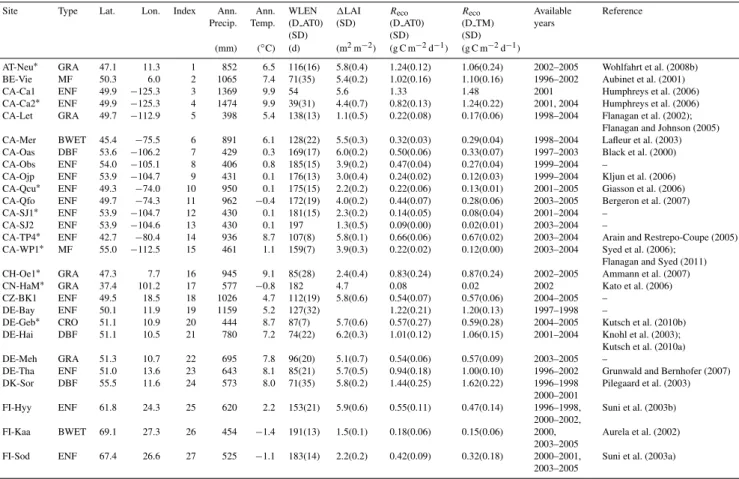
Figure 1 shows the frequency distribution of winter cumu-lativeReco and RWCR based on the two winter definitions D AT0 and D TM. These histograms contain data from all site-years. The winter cumulativeReco(g C m−2)for D TM and D AT0 ranges from 0.5 to 201.5 (median, 25th and 75th percentiles: 51.2, 24.1 and 78.0) and from 2.3 to 229.2 (64.8, 37.8 and 90.9), respectively. The RWCR (%) varies from 0.01 to 18.2 (5.3, 3.8 and 7.7) and from 0.7 to 22.5 (8.4, 5.9 and 10.4) for D TM and D AT0, respectively.
Winter Reco (g C m-2)
0 50 100 150 200 250
n
0 10 20 30 40 50
60 Mean: 54.8
Median: 51.2
n: 218 (a) D_TM
Winter Reco (g C m-2)
0 50 100 150 200 250
n
0 10 20 30 40 50
60 Mean: 71.2
Median: 64.8
n: 218 (b) D_AT0
RWCR (%)
0 5 10 15 20 25
n
0 10 20 30 40 50 60
70 Mean: 5.8
Median: 5.3 n: 218 (c) D_TM
RWCR (%)
0 5 10 15 20 25
n
0 10 20 30 40 50 60
70 Mean: 8.7
Median: 8.4
n: 218
(d) D_AT0 GRA
CRO ENF DBF MF BWET AWET
Fig. 1. Frequency histograms of winter cumulativeRecoand the ratio of winter cumulativeRecoto annual cumulativeReco(RWCR) (%) according to winter definition D TM (December–February) and D AT0 (air temperature<0◦C) across all of the site-years.nis the number of site years.
The RWCR (%) varies among ecosystem types (Table 2). Using definition D AT0, the highest RWCR values are found in both arctic and boreal wetlands and the lowest values in grasslands and croplands (Table 2). In contrast, when us-ing the D TM definition with a much shorter winter dura-tion in high latitudes, both arctic and boreal wetlands have a lower RWCR (Table 2). Compared to the RWCR, the RWRR (%) is less varied among different ecosystem types but shows a higher relative value for ecosystems with large permanent biomass such as forests, indicating the contribu-tion of autotrophic respiracontribu-tion. Arctic wetlands have much lower RWRR in D TM than D AT0, which can be related to the possibility that the microbial activity is much more con-strained by very low temperatures in D TM (Tsoil:−15.9◦C) than D AT0 (Tsoil: −11.3◦C). Similar to the RWCR, both croplands and grasslands have the relatively lower RWRR values (Table 2), which may be related to management prac-tices that remove the plant residuals fuelling winter respira-tion.
Except winter definition D TM, the RWCR increases with latitude (e.g. D AT0:r=0.33,p <0.05,n=57) since win-ter is often longer at higher-latitude sites (e.g. D AT0: r= 0.51,p <0.01). This pattern can be also found if grasslands and croplands are separated from forests (data not shown). The increase of the RWCR with latitude is not found in D TM due to its constant winter duration. These results
im-ply that winterReco in colder regions carries a higher rela-tive contribution to annual cumularela-tiveReco, due to its longer duration, than at warmer sites and thus further stresses the importance of winterRecofor the carbon balance of alpine, arctic and boreal ecosystems (e.g. Oechel et al., 1997; Fahne-stock et al., 1998; Bergeron et al., 2007; Wohlfahrt et al., 2008b). In this respect, we suggest that the established clima-tological winter season (December through February) should not be chosen to represent the role of winter time for an-nual carbon balances of seasonally cold sites. Due to sparse data for cold regions in global FLUXNET, the RWCR (4.9– 13.2 %) using D AT0 is on average lower in this study than in previous works (15–50 %) by Zimov et al. (1996) and Fahne-stock et al. (1998), focused on arctic ecosystems.
3.2 Temperature sensitivity of winterReco
3.2.1 Temperature sensitivity of winterRecoat the site level
Table 2.Summary statistics of mean winterRecorates (g C m−2d−1), winter cumulativeReco(g C m−2). RWRR values (%) and RWCR values (%) with winter definitions D AT0 (air temperature<0◦C) and D TM (December–February) across ecosystem types.
Vegetation type D AT0 D TM
Num Winter Length Winter cumulative Reco RWCR Mean Winter Reco rates
RWRR Num Winter
cumulative Reco RWCR Mean Winter Reco rates RWRR Mean (SD) Mean (SD) Mean (SD) Mean (SD) Mean (SD) Mean (SD) Mean (SD) Mean (SD) Mean (SD)
d (g C m−2) (%) (g C m−2d−1) (%) (g C m−2) (%) (g C m−2d−1) (%)
DBF 54 106ab(42) 89.0b(44.7) 8.9abc(4.0) 0.90c(0.39) 31.7b(11.6) 54 85.1c(42.7) 7.8b(3.1) 0.95c(0.47) 31.6b(12.7)
ENF 78 144ab(45) 76.3b(40.4) 9.9bc(3.9) 0.60bc(0.38) 26.0ab(8.4) 78 65.4bc(53.6) 6.2b(3.4) 0.73bc(0.60) 25.0b(13.9)
MF 17 113ab(44) 68.4b(33.4) 7.3ab(3.1) 0.70bc(0.33) 26.0ab(10.4) 17 67.5bc(35.8) 6.7b(3.3) 0.75bc(0.41) 27.1b(13.5)
GRA 33 114ab(29) 67.6b(50.1) 6.8ab(3.4) 0.62ab(0.43) 22.4ab(9.3) 33 50.0abc(34.7) 4.9ab(2.1) 0.56abc(0.39) 20.5b(8.5) CRO 20 93a(12) 45.3ab(20.8) 4.9a(1.9) 0.49abc(0.22) 19.4ab(7.5) 20 46.1abc(19.7) 5.0ab(1.9) 0.51abc(0.22) 20.3ab(7.9)
BWET 11 151b(37) 38.6ab(11.5) 10.8bc(3.7) 0.27ab(0.08) 25.8a(4.3) 11 21.6ab(7.6) 5.7b(1.1) 0.24ab(0.08) 23.1b(4.7)
AWET 5 248c(18) 6.0a(4.4) 13.2c(6.4) 0.02a(0.02) 19.5a(9.4) 5 1.1a(1.6) 1.7a(1.7) 0.01a(0.02) 6.8a(7.1)
ENF, DBF, MF, GRA, CRO, BWET and AWET represent evergreen needle leaf forests, deciduous broadleaf forests, mixed forests, grasslands, croplands, boreal wetlands and arctic wetlands, respectively.
RWCR and RWRR is the ratio of winter cumulativeReco(g C m−2)to annual cumulativeReco(g C m−2)and the ratio of mean winterRecorates (g C m−2d−1)to mean annual Recorates (g C m−2d−1), respectively.
SD is standard deviation. Mean (±1 SD) within a column followed by different letters (a, b and c) were significantly different (p <0.05).
Data normality was tested using one-sample Kolmogorov-Smirnov (K-S test) without the Dallal-Wilkinson-Lilliefor correction and the distribution of the data pooled from all of the site years is not significant from the normal distribution except winterRecorates in D TM (p=0.013,n=218). However, if K-S test with correction is used, the data in all of the cases did not conform to the normal distribution. We should thus take cautions about the existence of the risk of violation of assumptions of ANOVA.
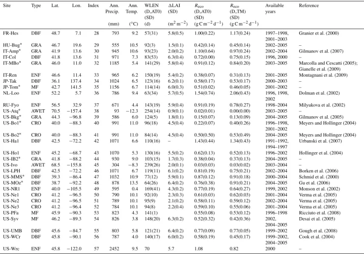
LAI (m2 m-2)
0 2 4 6
Reco
ref
(g C m
-2 d -1) 0.0 .5 1.0 1.5 2.0 2.5 2 3 4 7 8 9 10 11 12 13 14 15 21 23 24 25 27 33 28 31
34 35 36 37 4346 47 49 54 55 56 57 1 5 16 17 20 22 29 30 32 39 40 41 44 50 5152
Forest: r = 0.47, p < 0.01, n = 32
GRA+CRO: r = 0.37, p = 0.08, n = 16
(a) 0
∆
938
∆
Soil C density (kg C m-2)
0 5 10 15
Reco
ref
(g
C m
-2 d -1 ) .2 .4 .6 .8 1.0 1.2 1.4 1.6 2 7 8 9 11 19 21 25 27 33 42 43 47 55 56 r = 0.44, p = 0.097, n = 15
(b) 0
0 0 0
Soil C stock (kg C m
Soil C density (kg C m-2)
-2)0 5 10 15
Reco
ref
(g
C m
-2 d -1 ) .2 .4 .6 .8 1.0 1.2 1.4 1.6 2 7 8 9 11 19 21 25 27 33 42 43 47 55 56 r = 0.44, p = 0.097, n = 15
(b) 0
0 0 0
Soil C stock (kg C m
-2)
Fig. 2.The relationship between reference winter respiration (Recoref)calculated from the Arrhenius function and1LAI (m2m−2)(a)and total soil carbon stock (kg C m−2)(b)across sites. The site-specificR
ecorefis averaged from its site years, and its error bar is the standard deviation ofRecorefover the site-years. All values are calculated according to winter definition D AT0.
(Fig. 2a) (or GPP gs, data not shown) both in the forests and in grasslands and croplands. These results indicate that sub-strate availability, for which1LAI and GPP gs are taken as proxies, exerts a significant positive control onRecorefacross sites, and thus supports the conclusions of Grogan and Jonas-son (2005) who found thatRecorefwas significantly reduced after removing plant and litter in a birch and heath tundra. We also found thatRecorefis marginally correlated with total soil carbon stock in forest ecosystems (Fig. 2b). We did not perform the same analysis for grasslands and croplands due to their limited number of samples (n=5). Based on the for-est ecosystems our results support previous studies (Grogan et al., 2001; Nobrega and Grogan, 2007), which suggested that winter soil respiration is more derived from easier de-composable carbon (e.g. litter) than bulk soil organic matter
(SOC). This can be expected due to the fact that total soil carbon stock reflects the fraction of slow and passive com-pounds, which do not contribute much to Reco. However, SOC, which is buried beneath the active layer in frozen soils, has found to be labile and could be respired in case of per-mafrost thawing (Dutta et al., 2006; Nowinski et al., 2010). The decomposition of this old but labile SOC is of concern for future warming (on decadal scale), although this process is masked by the faster C cycling of fresh litter (on seasonal to interannual scale).
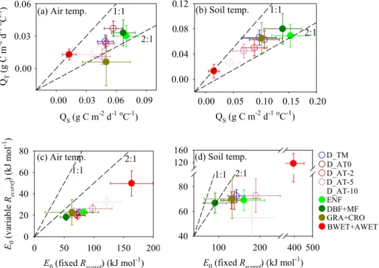
D_AT-10D_AT-5 D_AT0
ENF GRA D_TM D_AT-2
QS (g C m-2 d-1oC-1)
QT
(g C
m
-2 d
-1
o C
-1 ) (a) Air temp. 1:1
2:1
0.00 0.03 0.06 0.09 0.00
0.03 0.06
WET D_AT-10D_AT-5
D_AT0
DBF ENF GRA D_TM D_AT-2
QS (g C m -2
d-1oC-1) 0.00
.04 .08 .12
(b) Soil temp. 1:1
2:1
0 0 0
0.00 0.05 0.10 0.15 0.20
WET D_AT-10D_AT-5
D_AT0
DBF ENF GRA D_TM D_AT-2
E0 (fixed Recoref) (kJ mol-1)
0 50 100 150 200
E0
(v
ariab
le
Rec
o
re
f
) (kJ m
o
l
-1 )
0 20 40 60 80
(c) Air temp. 1:1
2:1
WET D_AT-10D_AT-5
D_AT0
DBF ENF GRA D_TM D_AT-2
E0(fixed Recoref) (kJ mol-1)
100 200 400 500
40 60 80 120 160
(d) Soil temp.
1:1 2:1
D_TM D_AT0 D_AT-2 D_AT-5 D_AT-10 ENF DBF+MF GRA+CRO BWET+AWET
Fig. 3.The winterRecosensitivity to temperature variation across space and the one over time is compared across different winter definitions and vegetation types, using both air(a)and soil(b)temperature, and two different types of winterRecosensitivity to temperature variation across space calculated from the Arrhenius function are also compared using both air(c)and soil(d)temperature. The values from vegetation type are calculated according to winter definition D AT0.
reduced if the soil reaches a critical freezing temperature (e.g. D AT0: US-Atq: −11.3◦C) in which microorganisms can be in a state of anabiosis (e.g.−10◦C in Vorobyova et al., 1997). In contrast, another arctic permafrost site (US-Ivo) had a comparably high activation energy (e.g. D AT0: 66.3 kJ mol−1)presumably due to higherTsoil (e.g. D AT0: −4.9◦C). Our understanding of winterR
ecocontrols in arc-tic permafrost regions is still very poor since only two per-mafrost sites are included in this study. This calls for further studies of different permafrost (e.g. continuous, discontinu-ous, and sporadic etc., Jorgenson et al., 2001; Zhang, 2005), vegetation types (e.g. Eugster et al., 2005) and in particular the different responses to freezing of oxic and anoxic systems underlain by permafrost.
3.2.2 WinterRecosensitivity to temperature variation over time
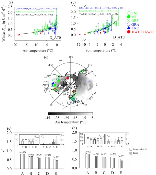
Our analysis shows that winterRecoanomalies positively cor-related with winter Tsoil anomalies, which explained more variability (e.g. D AT0:r=0.40,p <0.01,n=218; D TM: r=0.37, p <0.01, n=218, data not shown) than Tair (e.g. D AT0: r=0.30,p <0.01,n=218; D TM:r=0.22, p <0.01,n=218, data not shown). This is also found when using other winter definitions (data not shown). The ex-plained variance by the temperature is very low, but this
Air temperature (oC)
-20 -15 -10 -5 0
Wi
n
te
r
Rec
o
(g
C m
-2 d -1 )
0.0 .5 1.0 1.5 2.0 2.5
Forest (E0=75.5, Recoref=1.12, r=0.82, n=32)
Total (E0=74.8, Recoref=0.93, r=0.71, n=52)
GRA+CRO (E0=67.7, Recoref=0.67, r=0.41, n=16)
D_AT0 0
(a)
` 957
958 959 960 961 962 963 964 965 966 967 968 969 970 971 972 973 974 975 976
A
B
C
D
E
0.0
r
2
0.0
.5
1.0
1.5
2.0
A B C D E 0
100 200
A B C D E 0.3 0.6
0
E 0_air Aair
(n=32)
(n=32) (n=29) (n=25) (n=17)
(c)
** ** ** ** *
.
∆
A
B
C
D
E
0.0
0.0
.5
1.0
1.5
2.0
A B C D E 0
100 200 300
A B C D E 0.1 0.2
0
E 0_soil Asoil
(n=32)
(n=32) (n=29) (n=25) (n=17)
(d)
** ** ** ** **
.
Temp and LAI
Temp *
∆ Soil temperature (oC)
-12 -10 -4 -2 0 2 4
0.0 .5 1.0 1.5 2.0 2.5
Forest (E0=143.3, Recoref=0.61, r=0.79, n=32)
Total (E0=164.5, Recoref=0.56, r=0.71, n=52)
GRA+CRO (E0=185.3, Recoref=0.48, r=0.55, n=16)
D_AT0
ENF MF DBF GRA CRO
BWET+AWET
(b)
0
-45 -35 -25 -15 -5 5
-45 -35 -25 -15 -5 5
180
135 -135
-90
-45 30
60 90
(e)
Air temperature (oC)
Fig. 4. Relationships between winter air temperature(a), soil temperature(b)andRecousing winter definition D AT0. The coefficient of determination (r2)between the Arrhenius models with and without1LAI is compared using air temperature(c)and soil temperature(d)
respectively in the forest ecosystems. A, B, C, D, and E in both(c)and(d)denote winter definitions D TM, D AT0, D AT-2, D AT-5 and D AT-10, respectively. The spatial distribution of eddy covariance sites is displayed in(e). Winter air temperature from 1 December to 28 February is used as the background in(e). Significance levels are indicated as **, * and•representingp <0.01, 0.05 and 0.1, respectively.
3.2.3 The comparison between winterRecosensitivity to temperature variation across space and over time
Our analysis shows that the winterRecosensitivity to vari-ation ofTair orTsoil across space (QS; g C m−2d−1◦C−1),
defined as the slope of a linear regression between mean
all ecosystem types except boreal and arctic wetlands (Fig. 3a and b). No difference for the wetland (boreal and arctic wet-lands) category may be due to the low number of the samples in wetland (n=4). The same differences between the two temperature sensitivities can also be obtained if sites are cat-egorized by vegetation types according to other winter defi-nitions (data not shown).
The differences between these two winterReco tempera-ture sensitivities are due to the fact thatQT is mainly driven
by direct climate effects, butQS not only accounts for
gra-dients of climate affecting decomposition, but also reflects gradients in ecosystem state (e.g. soil C pools) in space (Hibbard et al., 2005) or the degree of adaptation of mi-croorganisms to low temperatures. To test this hypothesis, we regressed mean winterRecorates (g C m−2d−1)divided by site-specificRecoref provided by the within-site analysis (Sect. 3.2.1) against mean winterTairor Tsoil using the Ar-rhenius function. As shown in Fig. 3c and d, activation en-ergies (E0, kJ mol−1)were much smaller when using site-specific Recoref in all winter definitions and all vegetation types based on winter definition D AT0. This is consistent with the findings of recent studies (Mahecha et al., 2010; Wang et al., 2010), which showed that the temperature sen-sitivity (Q10)became much smaller after removing the in-fluence of confounding effects imposed by substrate avail-ability. Furthermore, from a multiple regression analysis conducted between mean winterReco rates and both mean winter temperature and1LAI (or GPP gs) across sites, we found thatQSbecame smaller if1LAI (or GPP gs) was
in-cluded (data not shown). For example, for winter defined as D AT0,QS (SD) calculated as a function of Tsoil changed from 0.11(0.03) to 0.08(0.03) after1LAI was included as an additional predictor. However, theQS after including1LAI
(D AT0: 0.08±0.03) remains larger than its corresponding QT (D AT0: 0.05±0.01), which can be expected due to the
possibility that1LAI only partly accounts for inter-site vari-ation in substrate availability (Sect. 3.2.1). This might imply thatQScan become closer toQT if spatial gradients in
sub-strates can be mostly taken into account.
The temperature sensitivity of respiration is a key param-eter controlling carbon-climate feedbacks in coupled mod-els (Friedlingstein et al., 2006). A fixed value of tempera-ture sensitivity, obtained from meta-analysis of spatial data (Raich and Schlesinger, 1992; Lloyd and Taylor, 1994) is often incorporated in these models (e.g. Cox et al., 2000; Friedlingstein et al., 2006). IfQS rather than QT is used
for winterReco, then, the current generation of models will likely overestimate the effect of future warming on soil C pools. However, great care should be taken into this extrap-olation when usingQT obtained from soil temperature. On
the one hand, in La Thuile dataset, the soil temperature mea-surement depth is not uniform across sites (the range is from 2 to 10 cm). On the other hand, the active layer where winter Recooccurs might be shallow and its depth might not neces-sarily coincide with the one for which soil temperature was
provided in the dataset. These two factors might contribute to the biased estimate of actual temperature response of win-terReco (e.g. Reichstein and Beer, 2008; Subke and Bahn, 2010).
3.3 Environmental and biotical controls on winterReco across sites
Since grasslands and croplands are heavily affected by hu-man hu-management on a short-term (e.g. seasonal and annual) basis, we conducted two separate cross site analyses, one for forests and the other for both grasslands and croplands. Wet-land sites were not included in the analysis since the number of the samples suited for our winterRecostudy in La Thuile dataset is too small (n=4).
Under all winter definitions, winter Reco is found to in-crease exponentially with increasing Tair andTsoil (Fig. 4a and b) across sites. On the basis of the aforementioned re-sults (Sect. 3.2.1), a linear dependence of the reference res-piration on1LAI or GPP gs was included (Eqs. 2 and 3). We only explored1LAI or GPP gs effects in the forest ecosys-tems since1LAI or GPP gs may be weak indicators of re-cent carbon inputs to the soil in grasslands and croplands (Fig. 2a), where much of the produced carbon is exported from the sites.
day 108 of year 2003, which is within the range of winter definition D AT0. In this respect, the role of winter precip-itation in regulatingRecois not as evident as in the growing season (e.g. Migliavacca et al., 2011). Second, winter snow-fall (solid precipitation) is one of many variables controlling snow depth, which was found to regulate Tsoil and micro-bial respiration under the snow pack when using Tair as a predictor of winterReco(e.g. Groffman et al., 2001, Grogan and Jonasson, 2006; Monson et al., 2006; Nobrega and Gro-gan, 2007). Snow depth is not simply related to winter snow-fall since it is influenced by local factors such as topography (e.g. Liston, 2004), wind speed (e.g. Li and Pomeroy, 1997), vegetation structure (e.g. Li and Pomeroy, 1997; Rutter et al., 2009), sublimation and melting. This justifies neglect-ing precipitation in our temperature response model (Eqs. 2 and 3).
Our results also showed that the inclusion of1LAI can only make a marginal improvement in winterRecoprediction of forest ecosystems (Fig. 4c and d), which was also observed if both total soil carbon stock and1LAI or GPP gs was in-cluded (data not shown). This may be related to the fact that aboveground respiration from tree biomass can still accounts for a significant fraction of winterReco(e.g. the reported val-ues are below 10 % or even higher than 50 %, Monson et al., 2005; Davidson and Janssens, 2006), thus reducing the fraction of heterotrophic respiration on winterRecousing the substrates such as litter. It would also suggest that both re-cent aboveground carbon inputs (approximated by1LAI or GPP gs) and soil carbon stock can not fully account for sub-strate availability (Fig. 2a and b), and belowground carbon inputs such as the senescence of fine roots and the supply of dissolved organic carbon or nitrogen (e.g. Edwards et al., 2006; Larsen et al., 2007) might play a role. Most notably, the substrates for winter soil respiration can be provided by the dead biomass of mycorrhizal fungi and other rhizospheric microbial cells that die at the autumn-winter transition period following the nighttime soil freezing.
4 Conclusions
The availability of meteorological and eddy covariance flux data across different ecosystems opens a new opportunity to quantify winter Reco and its spatial and temporal controls across North Hemisphere ecosystems. Given four different winter definitions, based on temperature below the freezing point, we found an increase in the ratio of winter to annual cumulative respiration towards higher latitude, due to the longer winters that occur at high latitudes. Therefore, due to the importance of winter processes in the carbon balance, it is important to better represent winterRecoin current ter-restrial carbon cycle models. The large number of sites now available provides an important source of information to im-prove winter carbon cycle. Our empirical characterization of temperature controls on winter Reco implies that winter
Recotemperature sensitivity obtained on spatial and temporal scales should be treated differently. The winterReco sensi-tivity to temperature variation across space (QS)was always
found to be higher than the one over time (QT)among
differ-ent winter definitions and among differdiffer-ent vegetation types except for the wetlands which had a limited sample size. Our result also imply thatQScan become closer to itsQT if
spa-tial gradients in inter-site substrates can be more and more taken into account. Thus, if extrapolated to future warming, the winterRecotemperature sensitivity to warming obtained from spatial gradients will be exaggerated without fully con-sidering the spatial difference in substrate availability.
Temperature is an overwhelming factor in determining the spatial variation of winterRecoin forests and grasslands and croplands. Although recent carbon inputs from aboveground marginally account for winterReco spatial variation, inter-site substrate availability (or biotic factors) does seem to be important since1LAI or GPP gs do partly account for the difference in reference respiration across sites. Indeed, the biotic controls of winterRecowere not fully explored in this study, which needs further investigation by considering be-lowground carbon inputs such as recently-killed rhizospheric microbial biomass and the senescence of fine roots. It should be noted that our results are mainly based on forest ecosys-tems and that winter carbon cycling in arctic ecosysecosys-tems with limited sample size in La Thuile dataset characterized by long winters and large soil carbon pools are still not well un-derstood. Furthermore, snow cover effects on winterReco were only explored using satellite-derived snow products, and these should be further investigated in future studies in which more in-situ snow data are available.
Acknowledgements. The authors would like to thank all the PIs of eddy covariance sites, technicians, postdoctoral fellows, research associates and site collaborators involved in FLUXNET who are not included as co-authors of the paper, without whose work this meta-analysis would not have been possible. This work is the outcome of the La Thuile FLUXNET workshop 2007, which would not have been possible without the financial support provided by CarboEurope-IP, FAO-GTOS-TCO, iLEAPS, Max Planck Institute for Biogeochemistry, National Science Foundation, University of Tuscia and the US Department of Energy. The Berkeley Water Cen-ter, Lawrence Berkeley National Laboratory, Microsoft Research eScience, Oak Ridge National Laboratory provided databasing and technical support. The AmeriFlux, AfriFlux, AsiaFlux, Car-boAfrica, CarboEuropeIP, ChinaFlux, Fluxnet-Canada, KoFlux, LBA, NECC, OzFlux, TCOS-Siberia, and USCCC networks provided data. We would also like to acknowledge the contribution of Larry Flanagan, who provides eddy covariance data of two sites (CA-WP1 and CA-Let) in Canada. We also acknowledge the Ph.D. funding by Commissariat `a l’´energie atomique (CEA) in France. Finally, we greatly thank the reviewers Werner Eugster, Thomas Friborg and other two anonymous reviewers for their constructive comments on the manuscript.
Appendix A
Table A1.WinterRecorates (g C m−2d−1)comparison among different winter definitions.
Site Type Lat. Lon. D TM D AT0 D AT-2 D AT-5 D AT-10
Reco WLEN Reco WLEN Reco WLEN Reco WLEN Reco
(SD) (SD) (SD) (SD) (SD) (SD) (SD) (SD) (SD)
(g C m−2d−1) (d) (g C m−2d−1) (d) (g C m−2d−1) (d) (g C m−2d−1) (d) (g C m−2d−1)
AT-Neu GRA 47.1 11.3 1.06(0.24) 116(16) 1.24(0.12) 92(32) 1.04(0.34) 62(22) 1.04(0.43) – – BE-Vie MF 50.3 6.0 1.10(0.16) 71(35) 1.02(0.16) 57(28) 0.89(0.15) 17 0.43 – –
CA-Ca1 ENF 49.9 –125.3 1.48 54 1.33 – – – – – –
CA-Ca2 ENF 49.9 –125.3 1.24(0.22) 39(31) 0.82(0.13) – – – – – – CA-Let GRA 49.7 –112.9 0.17(0.06) 138(13) 0.22(0.08) 120(21) 0.21(0.07) 100(32) 0.19(0.10) 61(37) 0.14(0.07) CA-Mer BWET 45.4 –75.5 0.29(0.04) 128(22) 0.32(0.03) 112(22) 0.30(0.04) 93(14) 0.28(0.04) 57(22) 0.24(0.03) CA-Oas DBF 53.6 –106.2 0.33(0.07) 169(17) 0.50(0.06) 157(21) 0.46(0.08) 141(13) 0.40(0.10) 101(18) 0.34(0.07) CA-Obs ENF 54.0 –105.1 0.27(0.04) 185(15) 0.47(0.04) 168(18) 0.42(0.04) 145(15) 0.35(0.06) 114(13) 0.30(0.03) CA-Ojp ENF 53.9 –104.7 0.12(0.03) 176(13) 0.24(0.02) 164(18) 0.21(0.04) 145(14) 0.17(0.05) 116(13) 0.14(0.03) CA-Qcu ENF 49.3 –74.0 0.13(0.01) 175(15) 0.22(0.06) 154(14) 0.19(0.04) 137(21) 0.17(0.05) 104(16) 0.12(0.01) CA-Qfo ENF 49.7 –74.3 0.28(0.06) 172(19) 0.44(0.07) 149(14) 0.39(0.07) 139(13) 0.37(0.05) 102(10) 0.30(0.04) CA-SJ1 ENF 53.9 –104.7 0.08(0.04) 181(15) 0.14(0.05) 172(19) 0.13(0.04) 146(20) 0.09(0.04) 121(8) 0.08(0.04) CA-SJ2 ENF 53.9 –104.6 0.02(0.01) 197 0.09(0.00) 167(4) 0.06(0.01) 137(17) 0.03(0.02) 123(7) 0.03(0.01) CA-TP4 ENF 42.7 –80.4 0.67(0.02) 107(8) 0.66(0.06) 99(8) 0.65(0.04) 61(30) 0.52(0.14) 19 0.43 CA-WP1 MF 55.0 –112.5 0.12(0.00) 159(7) 0.22(0.02) 155(6) 0.21(0.02) 143(16) 0.19(0.05) 103(28) 0.14(0.02) CH-Oe1 GRA 47.3 7.7 0.87(0.24) 85(28) 0.83(0.24) 58(13) 0.84(0.24) 43 0.73 – – CN-HaM GRA 37.4 101.2 0.02 182 0.08 159 0.06 148 0.06 98(12) 0.03(0.01) CZ-BK1 ENF 49.5 18.5 0.57(0.06) 112(19) 0.54(0.07) 105(22) 0.53(0.08) 47(1) 0.56(0.03) – – DE-Bay ENF 50.1 11.9 1.20(0.13) 127(32) 1.22(0.21) 77(30) 1.18(0.15) 91 1.11 – – DE-Geb CRO 51.1 10.9 0.59(0.28) 87(7) 0.57(0.27) 34(26) 0.45(0.12) – – – – DE-Hai DBF 51.1 10.5 1.06(0.15) 74(22) 1.01(0.12) 68(21) 1.01(0.14) 76 0.92 – – DE-Meh GRA 51.3 10.7 0.57(0.09) 96(20) 0.54(0.06) 81(4) 0.47(0.12) – – – – DE-Tha ENF 51.0 13.6 1.00(0.10) 85(21) 0.94(0.18) 53(29) 0.87(0.12) 48(38) 0.85(0.06) – – DK-Sor DBF 55.5 11.6 1.62(0.22) 71(35) 1.44(0.25) 63(33) 1.39(0.32) – – – – FI-Hyy ENF 61.8 24.3 0.47(0.14) 153(21) 0.55(0.11) 132(25) 0.50(0.13) 99(26) 0.44(0.13) 48(14) 0.42(0.13) FI-Kaa BWET 69.1 27.3 0.15(0.06) 191(13) 0.18(0.06) 182(9) 0.17(0.06) 147(16) 0.15(0.05) 100(19) 0.13(0.04) FI-Sod ENF 67.4 26.6 0.32(0.18) 183(14) 0.42(0.10) 166(9) 0.40(0.10) 146(15) 0.35(0.15) 113(11) 0.30(0.19) FR-Hes DBF 48.7 7.1 1.17(0.24) 57(31) 1.00(0.22) 55(28) 1.04(0.18) – – – – HU-Bug GRA 46.7 19.6 0.45(0.14) 92(3) 0.42(0.14) 67(25) 0.42(0.13) 33(26) 0.41(0.19) – – IT-Amp GRA 41.9 13.6 0.97(0.24) 93(23) 1.10(0.64) 43(32) 0.43(0.08) 24 0.23 – – IT-Col DBF 41.8 13.6 0.75(0.15) 83(53) 0.72(0.00) 101 0.67 – – – – IT-Mbo GRA 46.0 11.0 0.84(0.20) 141(29) 0.91(0.12) 98(19) 0.78(0.23) 68(37) 0.77(0.18) – – IT-Ren ENF 46.6 11.4 0.31(0.13) 150(19) 0.38(0.07) 118(21) 0.32(0.15) 58(35) 0.29(0.18) – – JP-Tak DBF 36.1 137.4 0.53(0.17) 123(16) 0.58(0.17) 94(11) 0.52(0.17) 77(7) 0.50(0.16) – – JP-Tom MF 42.7 141.5 0.46(0.05) 114(14) 0.51(0.02) 93(14) 0.47(0.03) 55(36) 0.46(0.06) – – NL-Loo ENF 52.2 5.7 2.06(0.43) 63(34) 1.54(0.74) 46(36) 1.41(1.02) 16 0.69 – – RU-Fyo ENF 56.5 32.9 0.78(0.27) 143(19) 0.91(0.19) 130(10) 0.86(0.21) 101(29) 0.81(0.25) 62(30) 0.62(0.15) US-Atq AWET 70.5 –157.4 0.00(0.00) 254(14) 0.02(0.01) 231(10) 0.01(0.00) 219(3) 0.01(0.00) 185(5) 0.01(0.00) US-Bkg GRA 44.3 –96.8 0.13(0.10) 124(5) 0.15(0.07) 117(0) 0.14(0.08) 104(14) 0.12(0.05) 59(35) 0.11(0.05) US-Bo1 CRO 40.0 –88.3 0.40(0.26) 96(18) 0.22(0.07) 69(28) 0.20(0.11) 31(10) 0.15(0.18) – – US-Bo2 CRO 40.0 –88.3 0.53(0.49) 84(14) 0.50(0.50) 68(29) 0.53(0.47) – – – – US-Ha1 DBF 42.5 –72.2 1.34(0.43) 110(16) 1.43(0.44) 88(3) 1.35(0.54) 59(13) 1.23(0.38) 32 1.19 US-Ho1 ENF 45.2 –68.7 0.52(0.13) 130(16) 0.62(0.13) 109(16) 0.53(0.10) 80(20) 0.46(0.11) 38(20) 0.29(0.05) US-IB2 GRA 41.8 –88.2 0.37(0.13) 103(15) 0.38(0.04) 67(28) 0.34(0.09) 60(29) 0.34(0.07) – – US-Ivo AWET 68.5 –155.8 0.03(0.02) 239(26) 0.03(0.03) 233(25) 0.03(0.02) 223(21) 0.02(0.02) 186(7) 0.02(0.01) US-LPH DBF 42.5 –72.2 0.75(0.21) 119(11) 0.81(0.19) 113(15) 0.79(0.20) 87(10) 0.74(0.19) 26(6) 0.62(0.28) US-MMS DBF 39.3 –86.4 0.91(0.18) 77(12) 0.87(0.12) 60(21) 0.84(0.12) 25(9) 0.75(0.21) – – US-Moz DBF 38.7 –92.2 0.91(0.21) 64(26) 0.76(0.38) 37 0.50 – – – – US-NR1 ENF 40.0 –105.5 0.64(0.27) 169(41) 0.77(0.19) 150(19) 0.73(0.24) 131(38) 0.70(0.22) 72 0.44 US-Ne1 CRO 41.2 –96.5 0.62(0.03) 92(10) 0.61(0.03) 73(25) 0.58(0.05) 57(17) 0.59(0.08) – – US-Ne2 CRO 41.2 –96.5 0.59(0.12) 95(9) 0.58(0.11) 79(22) 0.55(0.10) 52(17) 0.51(0.12) – – US-Ne3 CRO 41.2 –96.4 0.55(0.06) 94(8) 0.59(0.10) 79(17) 0.55(0.10) 58(17) 0.54(0.14) 18 0.32 US-PFa MF 45.9 –90.3 0.53(0.12) 141(1) 0.55(0.08) 137(1) 0.54(0.09) 112(24) 0.51(0.07) 44(17) 0.44(0.15) US-Syv MF 46.2 –89.3 0.42(0.36) 148(20) 0.52(0.32) 131(12) 0.43(0.36) 110(29) 0.40(0.33) 87(21) 0.32(0.44) US-UMB DBF 45.6 –84.7 0.77(0.05) 121(21) 0.77(0.09) 110(17) 0.76(0.09) 82(17) 0.71(0.08) 53 0.73 US-WCr DBF 45.8 –90.1 0.45(0.17) 140(17) 0.58(0.19) 118(23) 0.50(0.17) 101(17) 0.44(0.16) 73(11) 0.40(0.17)
US-Wrc ENF 45.8 –122.0 0.84 70 1.08 – – – – – –
Type: DBF: deciduous broadleaf forests; ENF: evergreen needleleaf forests; GRA: grasslands; CRO: croplands; BWET and AWET are boreal and arctic wetlands respectively; MF (mixed forests).
Lat. and Lon. are latitude and longitude, respectively. WLEN is the winter length (unit: day).
Recois mean winterRecorates (g C m−2d−1).
D AT0, D AT-2, D AT-5 and D AT-10 are defined as the period during which the 10 day smoothed air temperature remained below 0◦C,−2◦C,−5◦C and−10◦C for at least five
The publication of this article is financed by CNRS-INSU.
References
˚
Agren, G. I.: Temperature dependence of old soil organic matter, Ambio, 29, 55–55, 2000.
Ammann, C., Flechard, C. R., Leifeld, J., Neftel, A., and Fuhrer, J.: The carbon budget of newly established temperate grassland depends on management intensity, Agr. Ecosyst. Environ., 121, 5–20, doi:10.1016/j.agee.2006.12.002, 2007.
Arain, A. A. and Restrepo-Coupe, N.: Net ecosystem production in a temperate pine plantation in southeastern Canada, Agr. Forest Meteorol., 128, 223–241, doi:10.1016/j.agrformet.2004.10.003, 2005.
Aubinet, M., Chermanne, B., Vandenhaute, M., Longdoz, B., Yer-naux, M., and Laitat, E.: Long term carbon dioxide exchange above a mixed forest in the Belgian Ardennes, Agr. Forest Mete-orol., 108, 293–315, 2001.
Aurela, M., Laurila, T., and Tuovinen, J. P.: Annual CO2 bal-ance of a subarctic fen in northern Europe: Importbal-ance of the wintertime efflux, J. Geophys. Res.-Atmos., 107(D21), 4607, doi:10.1029/2002jd002055, 2002.
Baldocchi, D.: Breathing of the terrestrial biosphere: lessons learned from a global network of carbon dioxide flux measure-ment systems, Aust. J. Bot., 56, 1–26, 2008.
Baldocchi, D., Falge, E., Gu, L. H., Olson, R., Hollinger, D., Running, S., Anthoni, P., Bernhofer, C., Davis, K., Evans, R., Fuentes, J., Goldstein, A., Katul, G., Law, B., Lee, X. H., Malhi, Y., Meyers, T., Munger, W., Oechel, W., Paw U, K. T., Pilegaard, K., Schmid, H. P., Valentini, R., Verma, S., Vesala, T., Wilson, K., and Wofsy, S.: FLUXNET: A new tool to study the tem-poral and spatial variability of ecosystem-scale carbon dioxide, water vapor, and energy flux densities, B. Am. Meteorol. Soc., 82, 2415–2434, 2001.
Bergeron, O., Margolis, H. A., Black, T. A., Coursolle, C., Dunn, A. L., Barr, A. G., and Wofsy, S. C.: Comparison of carbon dioxide fluxes over three boreal black spruce forests in Canada, Glob. Change Biol., 13, 89–107, 2007.
Black, T. A., Chen, W. J., Barr, A. G., Arain, M. A., Chen, Z., Nesic, Z., Hogg, E. H., Neumann, H. H., and Yang, P. C.: Increased carbon sequestration by a boreal deciduous forest in years with a warm spring, Geophys. Res. Lett., 27, 1271–1274, 2000. Borken, W., Savage, K., Davidson, E. A., and Trumbore, S. E.:
Ef-fects of experimental drought on soil respiration and radiocarbon efflux from a temperate forest soil, Glob. Change Biol., 12, 177– 193, 2006.
Burba, G. G., Anderson, D. J., Xu, L., and McDermitt, D. K.: Addi-tional term in the Webb-Pearman-Leuning correction due to sur-face heating from an open-path gas analyzer, Eos Transactions AGU, 87(52), Fall Meeting Supplement, C12A-03, 2006. Burba, G. G., McDermitt, D. K., Grelle, A., Anderson, D. J., and
Xu, L. K.: Addressing the influence of instrument surface heat exchange on the measurements of CO2flux from open-path gas analyzers, Glob. Change Biol., 14, 1854–1876, 2008.
Clein, J. S. and Schimel, J. P.: Microbial Activity of Tundra and Taiga Soils at Subzero Temperatures, Soil Biol. Biochem., 27, 1231–1234, 1995.
Cook, B. D., Davis, K. J., Wang, W. G., Desai, A., Berger, B. W., Teclaw, R. M., Martin, J. G., Bolstad, P. V., Bakwin, P. S., Yi, C. X., and Heilman, W.: Carbon exchange and venting anomalies in an upland deciduous forest in northern Wisconsin, USA, Agr. Forest Meteorol., 126, 271–295, 2004.
Cox, P. M., Betts, R. A., Jones, C. D., Spall, S. A., and Totterdell, I. J.: Acceleration of global warming due to carbon-cycle feed-backs in a coupled climate model, Nature, 408, 184–187, 2000. Coyne, P. I. and Kelley, J. J.: Release of Carbon Dioxide from
Frozen Soil to Arctic Atmosphere, Nature, 234, 407–408, 1971. Davidson, E. A. and Janssens, I. A.: Temperature sensitivity of soil
carbon decomposition and feedbacks to climate change, Nature, 440, 165–173, 2006.
Desai, A. R., Bolstad, P. V., Cook, B. D., Davis, K. J., and Carey, E. V.: Comparing net ecosystem exchange of carbon dioxide be-tween an old-growth and mature forest in the upper Midwest, USA, Agr. Forest Meteorol., 128, 33–55, 2005.
Dolman, A. J., Moors, E. J., and Elbers, J. A.: The carbon uptake of a mid latitude pine forest growing on sandy soil, Agr. Forest Meteorol., 111, 157–170, 2002.
Dutta, K., Schuur, E. A. G., Neff, J. C., and Zimov, S. A.: Poten-tial carbon release from permafrost soils of Northeastern Siberia, Glob. Change Biol., 12, 2336–2351, 2006.
Edwards, K. A., McCulloch, J., Kershaw, G. P., and Jefferies, R. L.: Soil microbial and nutrient dynamics in a wet Arctic sedge meadow in late winter and early spring, Soil Biol. Biochem., 38, 2843–2851, 2006.
Eugster, W., McFadden, J. P., and Chapin, F. S.: Differences in sur-face roughness, energy, and CO2fluxes in two moist tundra veg-etation types, Kuparuk watershed, Alaska, USA, Arct. Antarct. Alp. Res., 37, 61–67, 2005.
Fahnestock, J. T., Jones, M. H., Brooks, P. D., Walker, D. A., and Welker, J. M.: Winter and early spring CO2efflux from tundra communities of northern Alaska, J. Geophys. Res.-Atmos., 103, 29023–29027, 1998.
Flanagan, L. B. and Johnson, B. G.: Interacting effects of temper-ature, soil moisture and plant biomass production on ecosystem respiration in a northern temperate grassland, Agr. Forest Mete-orol., 130, 237–253, 2005.
Flanagan, L. B. and Syed, K. H.: Stimulation of both photosynthesis and respiration in response to warmer and drier conditions in a boreal peatland ecosystem, Glob. Change Biol., 17, 2271–2287, 2011.
Flanagan, L. B., Wever, L. A., and Carlson, P. J.: Seasonal and inter-annual variation in carbon dioxide exchange and carbon balance in a northern temperate grassland, Glob. Change Biol., 8, 599– 615, 2002.
Friedlingstein, P., Cox, P., Betts, R., Bopp, L., Von Bloh, W., Brovkin, V., Cadule, P., Doney, S., Eby, M., Fung, I., Bala, G., John, J., Jones, C., Joos, F., Kato, T., Kawamiya, M., Knorr, W., Lindsay, K., Matthews, H. D., Raddatz, T., Rayner, P., Re-ick, C., Roeckner, E., Schnitzler, K. G., Schnur, R., Strassmann, K., Weaver, A. J., Yoshikawa, C., and Zeng, N.: Climate-carbon cycle feedback analysis: Results from the (CMIP)-M-4 model intercomparison, J. Climate, 19, 3337–3353, 2006.