Wind Turbine Micrositing: Comparison of Finite Difference
Method and Computational Fluid Dynamics
Samina Rajper1and Imran J. Amin2 1
Department of Computing, SZABIST Karachi, Sindh, Pakistan
2
Department of Computing, SZABIST Karachi, Sindh, Pakistan
Abstract
For smooth and optimal operation of wind turbines the location of wind turbines in wind farm is critical. Parameters that need to be considered for micrositing of wind turbines are topographic effect and wind effect. The location under consideration for wind farm is Gharo, Sindh, Pakistan. Several techniques are being researched for finding the most optimal location for wind turbines. These techniques are based on linear and nonlinear mathematical models. In this paper wind pressure distribution and its effect on wind turbine on the wind farm are considered. This study is conducted to compare the mathematical model; Finite Difference Method with a computational fluid dynamics software results. Finally the results of two techniques are compared for micrositing of wind turbines and found that finite difference method is not applicable for wind turbine micrositing.
Keywords: Wind farm, Finite Difference Method, Wind turbine micrositing, wind pressure, computational fluid dynamics.
1. Introduction
Arrhenius gave an idea about a century ago that emission of carbon dioxide from the fossil fuels will be the reason of Earth warming [1]. At present, the globe is looking for the alternate solutions instead of expensive and polluted fossil fuel or any other medium that discharge CO2. Unfortunately, Pakistan depends upon fossil fuels for producing electricity, which is costly and polluted source of energy. However, fossil fuel is one of the major imports of Pakistan to meet the energy requirements of country, as 64.12% of country’s total electricity production is obtained using fossil fuels [2]. Wind energy is used as the main source of producing electricity in many countries, such as Germany, Spain, United States, China, India [3].
At present, Wind turbine technology is the most mature and pollution free renewable technology available [4, 5]; because wind exists everywhere on the earth and it has been used as a source of mechanical energy for many
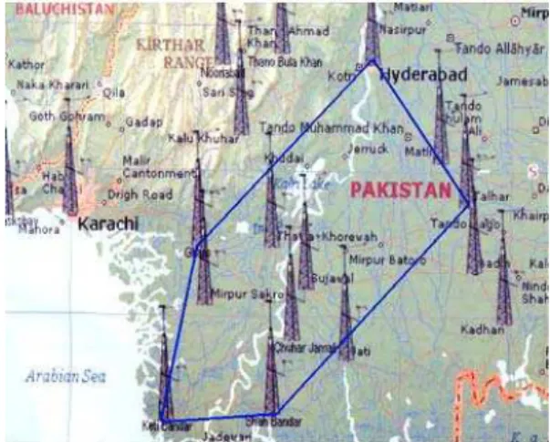
decades, furthermore there is a technological capacity also [5] .This study is conducted to optimize wind turbine micrositing. For this purpose, a research is being conducted to study wind pressure distribution and its effect on wind turbines, comparison between two techniques, i.e. computational fluid dynamics software VIZIFLOW 2.0 and discretized form of Laplace equation is made. The main objective of wind turbine micrositing is to gain the maximum result (net revenue) and to minimize the overall cost for energy. Systematical approach to wind turbine placement is a technical issue and was first been proposed by Moseti et al. and gradually worked and been improved by Grady et al.; genetic algorithm was used to find the optimal solution of the problem [6, 7]. Whereas, Computational fluid Dynamics techniques based on linear and nonlinear equations were used for the optimal placement of wind turbines in complex terrain [8]. The present study deals with the analysis of Gharo wind corridor which is the main site for installation of wind farm to meet the requirements of energy in Pakistan. Gharo, is a small town near the coast of Sindh, Pakistan. It is 1,046 Km long coastline, average wind speed is more than 7.4 m/s in Gharo and the estimated wind potential from this site is 50,000 MW [9, 10]. The site is shown in figure 1.
2. Methodology
divided into possible locations. To examine the concept only two Wind Turbines are supposed to be placed. The Diameter of wind turbine is supposed as 200 m. Therefore, the total area can be subdivided into 2kmx2km as shown in figure 3.
As the width supposed for each square grid/cell is good enough, the wake of a column of wind turbine should not affect another. As done in [11]. It is observed that 5D square grid size satisfies the Rule of Thumb spacing requirements for all vertical and horizontal directions [11]. Only one case is considered if the wind speed is constant at 10m/s and the direction of wind is from left to right, for the examining of Laplace equation. Same case is also examined using computational fluid dynamics software VIZIFLOW 2.0.
Fig. 1 Depicts the under consideration site Gharo, Thatta, Sindh.
Fig. 2 Represent the Methodology to compare two Techniques.
Fig. 3 200 m each cell for a square grid of 2kmx2km
3. Discretized form of Laplace Equation
The Laplace Equation is a second order partial differential equation (PDE). It is used in different areas of science and engineering for example in electricity, fluid mechanics etc. which is
+ =0 (1)
When the selection of a mathematical model is made, the next step is to select a suitable discretization method, i.e., a method of approximating the differential equations by a system of algebraic equations for the variables at some set of discrete locations in space and time. In a finite difference method, approximations for the derivatives at the grid points must be selected. Taylor series expansion is used to obtain approximations to the first and second derivatives of the variables with respect to the coordinates. When necessary, these methods are also used to obtain variable values at locations other than grid points. Here the Laplace equation is derived until and unless to the set of Linear i-e simultaneous equations [12]. A formal basis for developing finite difference approximation to derivative is by the use of Taylor series expansion. Because Taylor series expansion of a function f(x) is about a point x in the forward (positive x) and backward(negative x) directions given, similarly, for a point y upward (positive) and downward (negative) directions.
Assume that there are three points on the X-axis separated by a distance let h. Consider that I, i-1 and i+1 are center, left and right sides of the distance h. Similarly, for Y-axis j, j-1 and j+1 are center, downward and upward points. By applying Taylor expansions [12].
2 2 3 3 4 4
5
| | | | ( )
( 1) 2 2! 3 3! 4 4!
h h h
ih i i O h
i i x x x x
2 2 3 3 4 4 5
| | | | ( )
( 1) 2 2! 3 3! 4 4!
h h h
ih i i O h
i i x x x x
(3)
|i shows that the derivative is computed at the point i.
2
2 4 4 5
| | ( )
( 1) ( 1) 2 2 4 12
h
ih i O h
i i i x x
(4) 2 2 | 2 2 2
( 1) ( 1)
( )
i x
i i i
O h
h
(5)Subtracting equation (1) from equation (2), the resultant equation will be:
3 3
5
1 1
2
|
3|
3
(
)
i i
h
ih
i
o h
x
x
(6)Or
( 1) ( 1)
| ( 2)
2
i i
ih O h
x
h
(7)Applying same procedure to Y-axis, finally another equation will be:
2 2
|
2 2
2
( 1) ( 1)
( ) j y j O j j h
h
(8)( 1) ( 1)
| ( 2)
2
j j
jh O h
y
h
(9)By combining equations (7) and (9) the resultant equation for x and y will be:
2 2
) | ,
2 2
2 2
2 2
( 1), , ( 1), ,( 1) , ,( 1)
i j
x y
i j i j i j i j i j i j
h
h
(10)After substitution of equation (9) in Laplace equation the resultant equation will be:
1
, ( 1), ( 1), ,( 1) ,( 1)
4
i j i j i j i j i j
(11)
Or
( 1), ( 1), ,( 1) ,( 1)
4 ,
i j i j i
U U U j Ui j U i j
(12)
Assume that the x-axis and y-axis points i-e (i, j) are superposed then the resultant will be a 5- point pattern shown in figure 4.
Fig. 4 shows the position of points at x-axis and y-axis
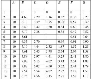
The Discretized form of Laplace equation is used to study the wind pressure distribution and its effect on the wind turbine on the wind farm . Here, the equation (12) shows that there are four variables represent the wind pressure on wind turbine and at different points as well to study the effects of wind pressure distribution. Based on equation 12 [12], air pressure distribution and its effects on wind turbine on the wind farm are considered. Initially, the effects are proven on MS Excel using Laplace equation then the Laplace equation’s discretized form is used for finite solution. The computed results based on discretized form of Laplace equation using MS Excel are depicted in table 1 and table 2. The air flow rate is constantly assumed as 10 m/s and using the discretized form of Laplace equation, the results are studied.
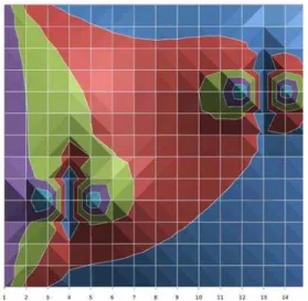
It is represented in table 1 and table 2 that cells D5, C6,D6,E6,D7 and M10,L11,M11,N11,M12 are supposed as 0 because the concept is to be examined that if the wind flows at constant speed and in the same direction on the wind turbine, what are wind pressure distribution effects. The mentioned cells of Excel sheet are the representation of wind turbine virtual existence. Suppose that cells D5,C6,D6,E6,D7 are wind turbine called “a” and cells M10,L11,M11,N11,M12 are named as “b”.It is depicted that results are satisfactory at wind turbine a but the results are not satisfactory when the same wind speed is applied to wind turbine b. As the wind pressure is gradually distributed and be slowed down if a wind turbine is there. The wind pressure at cells O11, N12 and N10 cannot be raised after it gets down to 0. Figure 7 is the MS-Excel Sheet results which are depicted by Table 1 and 2.
Figure 5 is the graphical representation of the results depicted earlier and represented by table 1 and table 2. There are two wind turbines are represented in figure 5. The wind pressure is assumed to be from left to right as shown in figure 5. It is shown in the figure 5 that the peaks are the high pressure points in the wind turbine. Table 3 depicts the computed results of wind turbine a and b. Later the effect of air pressure in mathematical model using finite difference method is compared with computational fluid dynamics software discussed in section 5.
4. Computational fluid Dynamics
A computational fluid dynamics software is used to compare the results of mathematical model with the results of computational fluid dynamics. The gauge theory of this software functions on the principles of two basic equations of fluid flow.
a) The continuity equation
A1v1=A2v2 (13)
Which means that the volume flow rate is constant, so that a smaller area for the fluid to flow will result in a higher velocity.
b) Bernoulli’s equation
This equation relates the pressure, flow velocity, fluid density and fluid height.
P1 + ρgy1 + ½ρv12 = P2 + ρgy2 + ½ρv22 (14)
The second term on each side of the equation represents the potential energy due to the height of the fluid, but since the height is constant in this cfd, these terms cancel and the equation reduces to:
P1 + ½ ρv12 = P2 + ½ρv22 (15)
P is the pressure, v the velocity and ρ the density of the fluid. To find the pressure P2 the equation is rearranged:
P2=½ρ(v22–v12)-P1 (16)
The wind flow is supposed as from left to right again. Table 4 is depicting the tested values for different attributes used for computational fluid dynamics software. Table 5 depicts wind pressure distribution effect is satisfactory at wind turbine a if the reading is taken at all points i.e. up, down, left and right of the turbine and the same procedure of taking readings is applied at wind turbine b. The computed results are not much different from wind turbine a and wind turbine b. The graphical representation of computed results using computational fluid dynamics software based on the discussed equation above as equation (13) and (16) is depicted using figure 6. The figure 6 also represents the same scenario with two wind turbines a and b, the blue color around the circles (virtual representation of wind turbines a and b) shows the high wind pressure.
Table 1: Results of wind speed pressure using Discretized form of Laplace equation on MS Excel.
A B C D E F G
1 0 0 0 0 0 0
2 10 4.60 2.29 1.16 0.62 0.35 0.23 3 10 6.10 3.39 1.75 0.95 0.57 0.39 4 10 6.40 3.42 1.50 0.84 0.60 0.48
5 10 6.10 2.38 - 0.33 0.49 0.52
6 10 5.61 - - - 0.51 0.64
7 10 6.35 2.70 - 0.69 0.91 0.90
8 10 7.10 4.44 2.52 1.87 1.52 1.25 9 10 7.61 5.45 3.78 2.74 2.07 1.58 10 10 7.89 5.97 4.41 3.25 2.41 1.80 11 10 7.98 6.15 4.62 3.43 2.54 1.87 12 10 7.88 6.02 4.50 3.32 2.44 1.79 13 10 7.54 5.54 4.02 2.92 2.12 1.53 14 10 6.75 4.56 3.15 2.21 1.58 1.13
A-Initial Wind Speed 10m/sec
Table 2: Depicts the continued results of wind speed pressure using Discretized form of Laplace Equation on MS Excel.
H I J K L M N O
1 0 0 0 0 0 0 0 0
2 0.23 0.16 0.12 0.10 0.08 0.06 0.04 0.03
3 0.39 0.30 0.24 0.19 0.15 0.11 0.08 0.05
4 0.48 0.40 0.33 0.27 0.22 0.16 0.12 0.07
5 0.52 0.49 0.43 0.35 0.28 0.21 0.15 0.09
6 0.64 0.61 0.54 0.44 0.34 0.25 0.17 0.11
7 0.90 0.80 0.66 0.52 0.39 0.27 0.18 0.11
8 1.25 1.01 0.80 0.60 0.42 0.28 0.17 0.10
9 1.58 1.21 0.91 0.65 0.43 0.25 0.12 0.07
10 1.80 1.34 0.97 0.67 0.41 0.16 - 0.02
11 1.87 1.37 0.98 0.65 0.35 - - -
Fig. 5 Wind turbines effect on Air pressure using Finite Difference Method
Fig. 6 Wind turbines effect on Air pressure using Computational fluid dynamics model (Two wind Turbines- a, b, Blue color shows high wind
pressure)
Table 3.Shows the Computed Results using Discretized form of Laplace Equation.
Wind-Turbine Position Flow Rate
a UP 1.5
Down 2.51
Left 5.61
Right 0.49
b UP 0.11
Down 0.06
Left 0.34
Right 0.00
Table 4 . Data for computational fluid Dynamics Test WT Flow
Rate
Pressur e
Densit y
Diameter Dist b/w WT 2 10
m/s
1 1 kg/
m3
20,20m,m 10 m
WT- Wind turbines
Table 5.Shows the Computed Results using computational fluid Dynamics.
Wind-Turbine Position Flow Rate
a UP 8.44
Down 6.42
Left 4.13
Right 4.91
b UP 6.79
Down 6.04
Left 2.65
Fig. 7 resulted Values on MS-EXCEL SHEET after using Laplace equation (Data is already given in Tables 1 and 2)
5. Discussion
In this paper, the study of wind turbine micro-siting using Finite Difference Method is represented. In this study wind pressure distribution and its effect on wind turbine on the wind farm are considered. Initially Laplace equation’s discretized form is used for finite solution. First the concept is proven on MS. Excel. Later the effect of air pressure in mathematical model using finite difference method is compared with computational fluid dynamics software. The computational fluid Dynamics software is based on another equation. The purpose was to study the wind air pressure distribution effects using two techniques. While using Technique 1; the result is depicted that if the wind speed is constant at 10m/s and direction is from left to right, the wind pressure distribution effect is computed at wind turbine a and wind turbine b are totally different from the results computed using the Technique 2.
The concept that the wind pressure will be less or even zero at the wind turbines and it gradually be raised to high pressure as it goes farther from wind turbines. This concept is proven positively at computational fluid dynamics however, this concept cannot be proved at Laplace equation. Using the Laplace equation, it is observed that when the wind pressure goes to zero it cannot be raised at the points where the wind pressure raised using computational fluid dynamics. Therefore, it is concluded that this model is not successful in comparison of computational fluid dynamics software (VIZIFLOW 2.0)based on the continuity equation and Bernoullis equation
Furthermore, Wind turbine placement is a discrete problem, therefore, classical methods are more complicated for optimization of this problem [13]. This study depicts that Mathematical model based on Laplace
equation in this study was initially tested using Excel sheet so it is suggested that it should be tested using Genetic algorithm to see the results. Because the Genetic algorithm technique operate on the coding of the parameter set rather than the parameter itself.
References
[1] I. Martin, et al , ‘Advanced Technology Paths to Global Climate Stability: Energy for a Greenhouse Planet’ a review in SCIENCE 298, 1, 2002
[2] Electrical Energy Sector Overview, Alternate Energy Development Board, Government of Pakistan, 2010 http://www.aedb.org/re_sector.php
[3] M. A. Ahmed, F. Ahmed and M. W. Akhtar, ‘wind characteristics and wind power potential for southern coasts of sindh, pakistan’, Journal of Basic and Applied Sciences, 6 (2), 163-168, 2010
[4] A. Houri, ‘Effects of Funds Diversion from Fuel Purchasing to Wind Energy Installations: A Case Study’ [5] J. F. Manwell, et al., ‘Wind Energy Explained : Theory ,
design and Application’ Second edition , Willey, published in 2009
[6] C. Wan, et al., ‘Optimal Micro-Siting of Wind Turbines by Genetic Algorithms Based on Improved Wind and Turbine Models’, Joint 48th IEEE Conference on Decision and Control
[7] S.A. Grady et al., “Placement of wind turbines using genetic algorithms”, Renewable Energy 30 (2005) 259–270 [8] J.M.L.M. Palma, ‘Linear and nonlinear models in wind
resource assessment and wind turbine micro-siting in complex terrain’, Journal of Wind Engineering and Industrial Aerodynamics, Volume 96, Issue 12, December 2008, Pages 2308-2326
[9] Saifullah, and A. Allauddin, ‘ Opportunities & Challenges toScaling up wind power in Pakistan’, Presentation in Quantum Leap in Wind Power in Asia Structured Consultation , June 21,22 2010
[10] Ch. Qamar-uz-Zaman et al., ‘Establishment of commercial wind power plant of 18 MW at Gharo’, Technical Report No. PMD-11/2004, pakistan meteorological department sector h-8/2, p. O. Box 1214, Islamabad
[11] G. Marmidis, et al., ‘Optimal placement of wind turbines in a wind park usingMonte Carlo simulation’, Renewable Energy 33 (2008) 1455–1460
[12] K. Ambar, ‘Finite Difference Method for the Solution of Laplace Equation’, Department of Aerospace Engineering Iowa State University