www.biogeosciences.net/13/1553/2016/ doi:10.5194/bg-13-1553-2016
© Author(s) 2016. CC Attribution 3.0 License.
Predicting biomass of hyperdiverse and structurally complex central
Amazonian forests – a virtual approach using extensive field data
Daniel Magnabosco Marra1,2,3, Niro Higuchi3, Susan E. Trumbore2, Gabriel H. P. M. Ribeiro3, Joaquim dos Santos3, Vilany M. C. Carneiro3, Adriano J. N. Lima3, Jeffrey Q. Chambers4, Robinson I. Negrón-Juárez5,
Frederic Holzwarth1, Björn Reu1,6, and Christian Wirth1,7,8
1AG Spezielle Botanik und Funktionelle Biodiversität, Universität Leipzig, Germany
2Biogeochemical Processes Department, Max Planck Institute for Biogeochemistry, Jena, Germany 3Laboratório de Manejo Florestal, Instituto Nacional de Pesquisas da Amazônia, Manaus, Brazil 4Geography Department, University of California, Berkeley, USA
5Climate Sciences Department, Lawrence Berkeley National Laboratory, Berkeley, USA 6Escuela de Biología, Universidad Industrial de Santander, Bucaramanga, Colombia
7German Centre for Integrative Biodiversity Research (iDiv) Halle-Jena-Leipzig, Leipzig, Germany 8Functional Biogeography Fellow Group, Max Planck Institute for Biogeochemistry, Jena, Germany Correspondence to:D. Magnabosco Marra ([email protected])
Received: 4 August 2015 – Published in Biogeosciences Discuss.: 18 September 2015 Revised: 23 February 2016 – Accepted: 26 February 2016 – Published: 11 March 2016
Abstract. Old-growth forests are subject to substantial changes in structure and species composition due to the in-tensification of human activities, gradual climate change and extreme weather events. Trees store ca. 90 % of the total aboveground biomass (AGB) in tropical forests and precise tree biomass estimation models are crucial for management and conservation. In the central Amazon, predicting AGB at large spatial scales is a challenging task due to the het-erogeneity of successional stages, high tree species diver-sity and inherent variations in tree allometry and architec-ture. We parameterized generic AGB estimation models ap-plicable across species and a wide range of structural and compositional variation related to species sorting into height layers as well as frequent natural disturbances. We used 727 trees (diameter at breast height ≥5 cm) from 101 genera and at least 135 species harvested in a contiguous forest near Manaus, Brazil. Sampling from this data set we as-sembled six scenarios designed to span existing gradients in floristic composition and size distribution in order to se-lect models that best predict AGB at the landscape level across successional gradients. We found that good individ-ual tree model fits do not necessarily translate into reliable predictions of AGB at the landscape level. When predict-ing AGB (dry mass) over scenarios uspredict-ing our different
1 Introduction
Allometries describe how relationships between different di-mensions (e.g., length, surface area and weight) of organ-isms change non-proportionally as they grow (Huxley and Teissier, 1936). The lack of proportionality arises from the fact that organisms change their shape while they grow (i.e., the dimensions differ in their relative growth rates). As one important application, allometric relationships can be used to relate simple dimensions of trees (e.g., diameter at breast height, DBH, or tree total height,H) to dimensions more rel-evant for forest managers and basic ecological research, such as wood volume or whole tree biomass (Brown et al., 1989; Higuchi et al., 1998; Saldarriaga et al., 1998).
Allometric relationships and biomass estimation models can differ substantially between different tree species, espe-cially in species-rich regions with a high variation in tree sizes and architectures such as in the tropical rainforests (Banin et al., 2012; Nelson et al., 1999; Poorter et al., 2003). This variation reflects differences in growth strategy and life history, such as tree species occupying different strata when mature (e.g., understory, canopy or emergent species), successional groups (SGs) (e.g., pioneer or light-demanding species, such as Cecropiaspp. andPouroumaspp., in con-trast to late-successional or shade-tolerant species, such as Cariniana spp. and Dipteryx spp.) or environmental mi-crosites (Clark and Clark, 1992; King, 1996; Swaine and Whitmore, 1988).
Important and highly variable architectural attributes of tropical tree species include stem shape (e.g., slender to stout form), branch form and branching intensity (e.g., pla-giotropic, orthotropic and unbranched), crown contour (e.g., round, elongated and irregular), crown position (e.g., under-story, canopy and emergent), maximum DBH andH (Hallé, 1974; Hallé et al., 1978). In addition, there is large varia-tion in growth rate (the speed at which a certain tree volume is filled) and consequently in wood anatomy among species (Bowman et al., 2013; da Silva et al., 2002; Worbes et al., 2003). Wood density (WD), which is particularly important for biomass estimation, varies significantly across regions (Muller-Landau, 2004) and can differ between species by more than an order of magnitude (Chave et al., 2006). Given these sources of variation, it is not surprising that different allometries were reported when comparing species (Nelson et al., 1999), successional stages (Ribeiro et al., 2014), on-togenies (Sterck and Bongers, 1998) and regions (Lima et al., 2012). Unfortunately, transferring such estimation mod-els to other contexts – other species, size ranges, life stages, sites or successional stages – typically leads to predictions that deviate strongly from observations, especially when the sampling design does not allow the selection of relevant data for proper estimation of the parameters of interest (Gregoire et al., 2016) or when predictor ranges are limited or neglected (Clark and Kellner, 2012; Sileshi, 2014).
In temperate and boreal forests, the size, ontogeny and site variations have been captured by the development of generic species-specific biomass estimation models (Wirth et al., 2004; Wutzler et al., 2008) based on data from hundreds of individuals from a single tree species. However, this ap-proach is prohibitive in the tropics where thousands of tree species coexist (Slik et al., 2015; ter Steege et al., 2013). In-stead, the challenge is to develop generic local or regional formulations that also generalize across species (Higuchi et al., 1998; Lima et al., 2012; Nelson et al., 1999; Saldarriaga et al., 1998). Ideally, they contain predictor variables that (1) jointly capture a large fraction of the variation induced by the underlying morphological and anatomical gradients and (2) are still easy enough to obtain or measure.
The development and application of such generic models pose a number of challenges. Finding the appropriate model structure and estimating the model parameters requires a data set with a large number of individual measurements contain-ing the variable of interest (here aboveground biomass, or AGB) and the predictor variables (i.e., DBH, H, species’ SGs and WD). Importantly, the data set should ideally cover all possible real-world combinations of predictor values in order to avoid error-prone extrapolations and unreliable dictions. However, in multiple regression models, this pre-condition is rarely met, not even by large design matrices.
The ultimate prediction is typically at the landscape level, which requires summing up individual predictions for several thousands of trees varying in size and species assignment. The larger the variation of predictor values within a stand, the higher is the likelihood that extrapolation errors occur. This calls for a validation at the landscape level, which requires a plot-based harvest method. For obvious reasons, this has rarely been attempted (Carvalho Jr. et al., 1995; Chambers et al., 2001; Higuchi et al., 1998; Lima et al., 2012).
Notable effort has already been made to parameterize global/pantropical AGB estimation models (Brown et al., 1989; Chave et al., 2005, 2014). Commonly, these mod-els are derived using several different data sets, each of which is comprised of relatively few trees and species. Al-though few opportunities exist to evaluate theses models at the landscape level, they are used worldwide in different con-texts, sites and across successional stages. For instance, the pantropical model from Chave et al. (2005) (DBH+WD as predictors) overestimated biomass when tested against trees in Gabon (Ngomanda et al., 2014), Peru (Goodman et al., 2014), Colombia (Alvarez et al., 2012) and Brazil (Lima et al., 2012), but it also underestimated the AGB in mixed-species Atlantic Forest stands in Brazil (Nogueira Jr. et al., 2014).
of old-growth forest can hold more than 280 tree species (DBH≥10 cm) (de Oliveira and Mori, 1999) with a wide range of architectures and anatomies (Braga, 1979; Muller-Landau, 2004; Ribeiro et al., 1999). At the landscape scale, this region encompasses a mosaic of successional stages promoted by windthrows (Asner, 2013; Chambers et al., 2013; Negrón-Juárez et al., 2010; Nelson et al., 1994). Dis-turbed areas include a diverse set of species representing the range from new regrowth to adult survivors, thereby in-cluding different SGs (pioneers, mid- and late-successional species), tree sizes and with a broader range of architec-tures than old-growth forests (Chambers et al., 2009; Marra et al., 2014; Ribeiro et al., 2014). Once floristic composi-tion changes and structural gradients increase to this extent, allometry becomes more complex and reliable landscape-level biomass estimates rely on designed and well-tested generic biomass models.
We report here a novel data set of 727 trees harvested in a contiguous terra firme forest near Manaus, Brazil. This data set includes biomass measurements from 101 genera and at least 135 tree species that vary in architecture and are from different SGs (pioneers, mid- and late successional). These trees span a wide range of DBH (from 5 to 85 cm),H (from 3.9 to 34.5 m) and WD (from 0.348 to 1.000 g cm−3). We used this data set to parameterize generic AGB estimation models for central Amazonian terra firme forests applicable across species and a wide range of structural and composi-tional variation (i.e., secondary forests), using various sub-sets of the available predictors; i.e., size (DBH andH ), SGs and WD.
We next evaluated our models, as well as the pantropical model from Chave et al. (2014) at the landscape level using a virtual approach. We created scenarios of simulated 100 1 ha forest plots by assembling subsets of the 727 known-biomass trees in our data set. These scenarios were designed to span gradients in (1) floristic composition, by assembling stands with specific proportions of pioneer, mid- and late-successional species, and (2) size distributions of trees. We compared the known biomass of these forest assemblage sce-narios to predictions based on the generic models, with the goal of answering the following questions.
1. Which variance modeling approach and combinations of predictors produced the best individual tree biomass estimation model?
2. Which model most reliably predicted AGB at landscape level, i.e., across successional gradients?
We expected that the best model, the one reducing both mean deviation and error of single and landscape-level biomass prediction, would require species-specific variables as well as an additional parameter allowing the modeling of het-eroscedastic variance. Our approach and the independence of our data set allowed us to evaluate whether it is still im-portant to build local/regional models or whether available
pantropical/global models are suitable for landscape biomass assessments – under the assumption that they predict biomass satisfactorily over all sorts of tropical forest types and succes-sional stages.
2 Material and methods 2.1 Study site
Our study site is located at the Estação Experimental de Silvi-cultura Tropical (EEST), a 21 000 ha research reserve (Fig. 1) managed by the Laboratório de Manejo Florestal (LMF) of the Brazilian Institute for Amazon Research (INPA), Man-aus, Amazonas, Brazil (2◦56′S, 60◦26′W). Averaged annual temperature in Manaus was 26.7◦C for the 1910–1983 pe-riod (Chambers et al., 2004). Averaged annual precipitation ca. 50 km east of our study site was 2610 mm for the 1980– 2000 period (da Silva et al., 2003) with annual peaks of up to 3450 mm (da Silva et al., 2002). From July to September there is a distinct dry season with usually less than 100 mm of rain per month. Topography is undulating with elevation ranging from ca. 50 to 140 m a.s.l. Soils on upland plateaus and the upper portions of slopes have high clay content (Ox-isols), while soils on slope bottoms and valleys have high sand content (Spodosols) and are subject to seasonal flood-ing (Telles et al., 2003). In contrast to floodplains (i.e., igapó and várzea) associated with large Amazonian rivers (e.g., Rio Negro and Rio Amazonas), valleys associated with streams and low-order rivers can be affected by local rain events and thus have a polymodal and unpredictable flood-pulse pattern with many short and sporadic inundations mainly during the rainy season (Junk et al., 2011).
The EEST is mainly covered by a contiguous closed canopy old-growth terra firme forest with high tree species diversity and dense understory (Braga, 1979; Marra et al., 2014). The terra firme forests are among the predominant forest types in the Brazilian Amazon (Braga, 1979; Higuchi et al., 2004) and ca. 93 % of the total plant biomass is stored in trees with DBH≥5 cm (Lima et al., 2012; da Silva, 2007). The tree density (DBH≥10 cm) in the EEST is 593± 28 trees ha−1 (mean±99 % confidence interval) (Marra et al., 2014). Trees larger than 100 cm in DBH are rare (< 1 in-dividual ha−1) and those with DBH > 60 cm accounted for only 16.7 % of the AGB (Vieira et al., 2004). In the study region, tree mortality rates can be influenced by variations in topography (Marra et al., 2014; Toledo et al., 2012). Floristic composition and species demography can also vary with the vertical distance from drainage (Schietti et al., 2013). 2.2 Allometric data
Figure 1.Study site of terra firme forest near Manaus, Amazonas, Brazil.
are given in Table S1 in the Supplement). The trees were harvested through the plot-based harvest method in an old-growth forest and in two contiguous secondary forests (14-year-old regrowth following slash and burn and 23-(14-year-old regrowth following a clear cut) (Fig. 1). Rather than an indi-vidual selection, our plot-based method relies on the harvest-ing of all trees found in selected plots. This method allows for a valid/faithful representation of the DBH distribution of the target forests and a landscape validation of the fitted models (Higuchi et al., 1998; Lima et al., 2012).
Before selecting plots, we surveyed both the old-growth and secondary forests to assure that no strong differences in structure and floristic composition existed and that the se-lected patches were representative of our different succes-sional stages. In the old-growth forest the trees were har-vested in eight plateau and three valley plots (10 m×10 m) randomly selected within an area of 3.6 ha (da Silva, 2007). In each of the secondary forests the trees were harvested in five plots (20 m×20 m), each randomly selected within a 1 ha plateau area (dos Santos, 1996; da Silva, 2007). By in-cluding trees from secondary forests we were able to increase the variation in floristic composition and consequently the range of species-related variation in architecture and allome-try (Table 1 and Table S1). Since our secondary forests were inserted in the contiguous matrix from which old-growth plots were sampled, we also controlled for the effects of im-portant drivers of tree allometry and architecture, such as variations in environmental conditions (e.g., soil, precipita-tion rates and distribuprecipita-tion), forest structure and wood density (Banin et al., 2012); the last is intrinsically related to varia-tion in floristic composivaria-tion.
Table 1.Summary of the data set applied in this study. Trees were harvested in the Estação Experimental de Silvicultura Tropical, a contiguous terra firme forest reserve near Manaus, Amazonas, Brazil.
Variables Old-growth Secondary forest Secondary forest forest (23 years old) (14 years old)
NT 131 346 250
SR 82 63 51
DBH 5.0–85.0 5.0–37.2 5.0–33.1
H 5.9–34.5 3.9–27.0 9.0–15.5
WD 0.348–0.940 0.389–1.000 0.395–1.000 AGB 8.3–7509.1 5.4–1690.2 7.5–1562.8
Variables: number of trees (NT), species richness (SR), diameter at breast height (DBH) (cm), tree total height (H )(m), wood density (WD) (g cm−3)and aboveground biomass (AGB) (dry mass in kilograms).
Trees were harvested at ground level. For each tree, the DBH (cm),H (m) and fresh mass (kg) were recorded in the field by using a diameter tape, a meter tape and a mechani-cal metal smechani-cale (300 kg×200 g), respectively. The DBH was measured before, while H was measured after harvesting. For trees with buttresses or irregular trunk shape, the di-ameter was measured above these parts. Each tree compo-nent (i.e., stem, branches and leaves) was weighted sepa-rately. For large trees, stems were cut into smaller sections before weighing. The mass of sawdust was collected and weighted together with its respective stem section. Leaves and reproductive material, when available, were collected to allow species identification accordingly to the APGIII sys-tem (Stevens, 2012). Botanical samples were incorporated in the EEST collection. The water content for each tree was determined from three discs (2–5 cm in thickness), collected from the top, middle and bottom of the bole, and samples (ca. 2 kg) of small branches and leaves. The samples were oven dried at 65◦C to constant dry mass. The dry mass data were calculated by using the corresponding water content of each component (Lima et al., 2012; da Silva, 2007). Dry mass for each tree was used for subsequent model fits and compar-isons.
2.3 Species’ architecture attributes
et al., 2014) and species descriptions available in the Mis-souri Botanical Garden (http://www.tropicos.org), species-Link (http://www.splink.cria.org.br) and Lista de Espécies da Flora do Brasil (http://www.floradobrasil.jbrj.gov.br/). More importantly, we considered empirical field observations, ar-chitectural information from our data set and data for species presence/absence from a network of permanent plots repre-senting a wide range of successional stages in central Ama-zon (Table S2). This network includes plots in old-growth forests (LMF unpublished data (census from 1996 to 2012); da Silva et al., 2002), secondary forests (Carvalho Jr. et al., 1995; dos Santos, 1996), and small and large canopy gaps (≥ ca. 2000 m2)created by windthrows that are 4, 7, 14, 17, 24 and 27 years old (LMF unpublished data; Marra et al., 2014). Since reported WD values for the same species or gen-era can vary strongly among different studies (Chave et al., 2006) and sites (Muller-Landau, 2004), we compiled WD values mainly from studies carried out in the Brazilian Ama-zon (Chave et al., 2009; Fearnside, 1997; Laurance et al., 2006; Nogueira et al., 2005, 2007). For species where WD data were not available for the Brazilian Amazon, we con-sidered studies from other Amazonian regions (Chave et al., 2009). For species where no published WD was available, or where the identification was carried out to the genus level (63 in total), we used the mean value for all species from the same genus occurring in central Amazon. For trees iden-tified only to the family level (seven in total), we used the mean value of genera from that family excluding those not reported in the study region (Table S1).
2.4 Statistical analyses
2.4.1 Individual tree biomass estimation model fits The AGB estimation models we applied varied in the num-ber and combination of our predictor variables (eight combi-nations/series) as well as the strategy of modeling the vari-ance (three model types – see below), yielding a set of 24 candidate models (Table 2). We used DBH (cm), WD (g cm−3)andH(m) as predictors. Furthermore, we used the species’ SG assignment as a “categorical predictor” (factor 1 is pioneer, 2 is mid-successional and 3 is late-successional species), thereby representing functional diversity along a main axis of tree successional strategies, functional and ar-chitectural variation. Depending on the model-type parame-ters, the continuous variables were allowed to vary for cap-turing the successional aspects of functional diversity. We consider the SG grouping factor as integral part of the model. Fitting all SGs in one model in an Markov chain Monte Carlo context is different than fitting separate models because the joint model also absorbs the covariance structure of the pa-rameters across groups, especially in models where not all parameters are allowed to vary among SGs.
We tested variables for collinearity by calculating the vari-ance inflation factor (VIF). A conservative VIF > 2.0
in-dicates significant collinearity among variables (Graham, 2003; Petraitis et al., 1996). Model series 1–4 had VIF < 1.5 (Table 2), which indicated no significant collinearity among predictors. For model series 5–8, we found VIF > 2.0 for DBH andH, which indicates significant collinearity between these two variables. This pattern was previously reported for other data sets from Amazon and other tropical regions (Lima et al., 2012; Ribeiro et al., 2014; Sileshi, 2014).
We fit models representing the eight different predictor combinations to our entire data set of 727 trees using three variance modeling approaches: nonlinear least square (NLS), ordinary least square with log-linear regression (OLS) and a nonlinear approach in which we modeled the heteroscedastic variance of the data set (MOV). In the MOV approach we modeled the variance as a function of DBH with a normally distributed residual error:
εi =N yˆi, σi
, (1)
whereiis the subscript for individuals (i=1, ...,n) andσiis modeled with a heteroscedastic variance according to
σi=ci·DBHci2. (2)
Model series 1 (M11, M12 and M13) used DBH as the sole predictor (Table 2). For model series 2 (M21, M22 and M23), we allowed thebregression parameters andc heteroscedas-tic variance to vary according to the SG assignment (1, 2 or 3). This approach allowed us to account for differences among the SGs without splitting the data set into three differ-ent groups. This method has increased analytical power and allowed us to assess the relationships between tree allometry and architecture.
For model series 3 (M31, M32 and M33), we ignored the SG assignment but introduced WD (which did not correlate strongly with SG). For model series 4 (M41, M42 and M43) we allowed each SG to have its own wood density effect. For model series 5 and 6, we replaced the WD withH. In model series 5 (M51, M52 and M53), we restricted the SG variation of b and c, while in series 6 (M61, M62 and M63) we allowed these parameters to vary according to SG. For model series 7 (M71, M72 and M73), we combined DBH,H and WD but restricted the SG variation ofbandc. Finally, for model series 8 (M81, M82 and M83), we combined DBH,H and WD and allowedbandcto vary with SG (Table 2).
In contrast to prior approaches, we did not test mod-els based on compound (e.g., log[AGB] ∼ log[b1] +
b2[logDBH2HWD]) or quadratic/cubic derivatives (e.g., log[AGB] ∼ log[b1] + b2[logDBH] + b3[logDBH2] +
b4[logDBH3]) (Brown et al., 1989; Chave et al., 2005, 2014; Ngomanda et al., 2014). These structures would have limited our ability to include biological variation by defining SG-specific parameters for DBH,Hand WD separately.
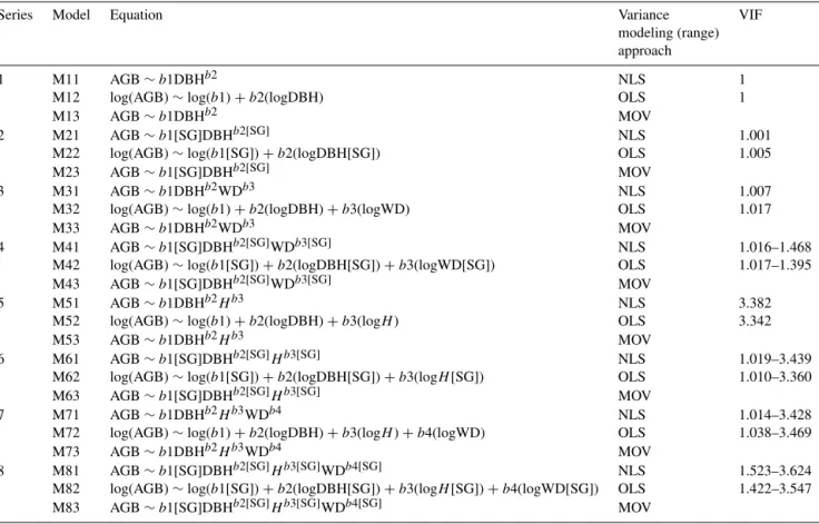
Table 2.Tested equations for estimating aboveground tree biomass (AGB) in a terra firme forest near Manaus, Amazonas, Brazil.
Series Model Equation Variance VIF
modeling (range) approach
1 M11 AGB∼b1DBHb2 NLS 1
M12 log(AGB)∼log(b1)+b2(logDBH) OLS 1
M13 AGB∼b1DBHb2 MOV
2 M21 AGB∼b1[SG]DBHb2[SG] NLS 1.001
M22 log(AGB)∼log(b1[SG])+b2(logDBH[SG]) OLS 1.005
M23 AGB∼b1[SG]DBHb2[SG] MOV
3 M31 AGB∼b1DBHb2WDb3 NLS 1.007
M32 log(AGB)∼log(b1)+b2(logDBH)+b3(logWD) OLS 1.017
M33 AGB∼b1DBHb2WDb3 MOV
4 M41 AGB∼b1[SG]DBHb2[SG]WDb3[SG] NLS 1.016–1.468
M42 log(AGB)∼log(b1[SG])+b2(logDBH[SG])+b3(logWD[SG]) OLS 1.017–1.395
M43 AGB∼b1[SG]DBHb2[SG]WDb3[SG] MOV
5 M51 AGB∼b1DBHb2Hb3 NLS 3.382
M52 log(AGB)∼log(b1)+b2(logDBH)+b3(logH) OLS 3.342
M53 AGB∼b1DBHb2Hb3 MOV
6 M61 AGB∼b1[SG]DBHb2[SG]Hb3[SG] NLS 1.019–3.439
M62 log(AGB)∼log(b1[SG])+b2(logDBH[SG])+b3(logH[SG]) OLS 1.010–3.360
M63 AGB∼b1[SG]DBHb2[SG]Hb3[SG] MOV
7 M71 AGB∼b1DBHb2Hb3WDb4 NLS 1.014–3.428
M72 log(AGB)∼log(b1)+b2(logDBH)+b3(logH)+b4(logWD) OLS 1.038–3.469
M73 AGB∼b1DBHb2Hb3WDb4 MOV
8 M81 AGB∼b1[SG]DBHb2[SG]Hb3[SG]WDb4[SG] NLS 1.523–3.624
M82 log(AGB)∼log(b1[SG])+b2(logDBH[SG])+b3(logH[SG])+b4(logWD[SG]) OLS 1.422–3.547 M83 AGB∼b1[SG]DBHb2[SG]Hb3[SG]WDb4[SG] MOV
Predictors: diameter at breast height (DBH) (cm), species’ successional group (SG) (pioneers, mid- and late successional), tree total height (H )(m) and wood density (WD) (g cm−3). Variance modeling approach: nonlinear least square (NLS), ordinary least square with log-linear regression (OLS) and nonlinear with modeled variance (MOV).
Since NLS and MOV rely on the same equation, they have analogue variation inflation factor values (VIF).
run in parallel, and convergence of the posterior distribution for each parameter was assessed by convergence of the ratio of pooled to mean within-chain central 80 % intervals to 1 or by the stability of both intervals (Brooks and Gelman, 1998; Brooks and Roberts, 1998).
To select the best model we calculated the deviance information criterion (DIC). The DIC is a generalization of Akaike’s information criterion and consists of a cross-validatory term that expresses both the goodness of the fit and the models’ complexity. The lower the value the higher the predictive ability and parsimony (Spiegelhalter et al., 2002). We also checked whether the 95 % credible intervals of the parameter’s posterior distributions excluded 0. However, we did not attempt to test the null hypothesis that a particular parameter is 0 (Bolker et al., 2013; Bolker, 2008). Contrasts were evaluated by monitoring differences between parame-ters or predictions based on their posterior distribution. For communicating the results we consider two parameters sig-nificantly different if the 95 % credible interval of the poste-rior distribution of their difference does not include 0.
To allow for comparisons of different model structures and approaches with the available literature, we calculated the coefficient of determination (R2), the adjusted coefficient of
determination (R2adj) and the relative standard error (Syx%).
TheSyx%was calculated as follows: Syx%=
2s
ˆ
y√N
, (3)
wheres,yˆandNare the standard deviation of the regression, the mean of the focal independent variable and the number of observations, respectively. As in all allometric data sets relating linear to volume-proportional data, there is indeed heteroscedasticity in our data, which restricts the use of the
Syx% for model selection. Nonetheless, this measure is
pre-scribed for assessing models’ uncertainty (IPCC, 2006) and is commonly used (Chave et al., 2014; Lima et al., 2012; Ribeiro et al., 2014; Sileshi, 2014).
For the OLS approach including log-transformed vari-ables, we calculated theSyx% using untransformed data. To
correct for the bias introduced by the log-transformed data, a correction factor (CF) was calculated as follows:
CF=exp SSE
2
2 !
, (4)
Figure 2. Sampling schemes applied to assemble the six forest scenarios designed to reflect changes in floristic composition and size distribution of trees, typical of central Amazonian terra firme forests.
2.5 Landscape-level biomass predictions across scenarios
To evaluate the models outlined in Table 2, we predicted AGB at the landscape level for six forest scenarios assembled by a stratified random selection of individual trees from our data set of 727 trees. Our scenarios were designed to span a successional gradient created by natural disturbances in which the interaction of tree mortality intensity and species vulnerability and resilience produce complex communities varying in species composition and size distribution of trees (Chambers et al., 2009, 2013; Marra et al., 2014). We as-sembled three scenarios to reflect variations in floristic com-position and three scenarios to reflect variations in size dis-tribution. Each scenario was sampled 100 times, resulting in 100 1 ha plots per scenario with different combination of trees randomly (with replacement) assembled according to the scenario-specific design principles.
To address the effect of variations in floristic composition on estimated AGB, we created scenarios where we varied the proportion of pioneer, mid- and late-successional species. The early-successional scenario comprised 50 % from trees sampled randomly from the species classified as pioneer, 40 % from mid- and 10 % from late-successional species (as survivors of disturbances). The mid-successional sce-nario comprised 10 % from trees sampled randomly from the species classified as pioneer, 70 % from mid- and 20 % from late-successional species. The late-successional sce-nario comprised 10 % from trees sampled randomly from the species classified as pioneer, 40 % from mid- and 50 % from late-successional species (Fig. 2a and c). We
con-strained our floristic composition scenarios to a stem density of 1255 trees ha−1(DBH≥5 cm) typical for the old-growth terra firme forests at the EEST (Lima et al., 2007; Marra et al., 2014; Suwa et al., 2012).
To address variations in size distribution, we varied the proportion of small and big trees fixing a threshold value of 21 cm, which represents the mean DBH (trees with DBH≥10 cm) of our studied forest (Marra et al., 2014). Our size-distribution scenarios included a small-sized stand, with 90 % from small (DBH < 21 cm) and 10 % from big trees (DBH≥21 cm); a mid-sized stand with equal numbers of trees smaller and greater than or equal to 21 cm in DBH; and a large-sized stand, with 10 % small and 90 % big trees (Fig. 2b and d). As for our floristic composition scenarios, in order to produce reliable size-distributions, we constrained our sampling effort to a basal area value of 30.3 m2ha−1 also typical of our studied old-growth forest (trees with DBH≥5 cm) (Marra et al., 2014; Suwa et al., 2012). Both our floristic and size-distribution scenarios produced theJ -inverse distribution pattern, typical of tropical forests (Clark and Clark, 1992; Denslow, 1980).
AGB at the landscape level was determined by adding up the measured AGB for “sampled” trees in each scenario. To test how well our biomass estimation models predicted the AGB at the stand level, we related biases and root-mean-square error (RMSE). In order to assess the accuracy of dif-ferent predictions in the context of models’ uncertainty, we additionally reported the overall performance of the tested models along all forest scenarios. When doing so, we present the bias and RMSE in the same unit (Mg), which allow for assessing the magnitudes of deviations in model predictions (Gregoire et al., 2016; McRoberts and Westfall, 2014). Be-cause data on tree height are normally unavailable or esti-mated imprecisely in Amazonian forest inventories, we fo-cused on models including only DBH, WD and SG as pre-dictors (model series 1–4). In addition to the “internal eval-uation” of our models, we tested the pantropical model from Chave et al. (2014):
\
logAGB∼ −1.803−0.976E+0.976 logWD
+2.673
logDBH
−0.0299[logDBH]2, (5) which was parameterized with data from 4004 trees (DBH≥5 cm) harvested in 53 old-growth and five secondary forests. This model has DBH,H(estimated from a DBH :H
relationship), WD and a variableE(environmental stress) as predictors and was suggested for estimating tree AGB in the absence of height measurements.
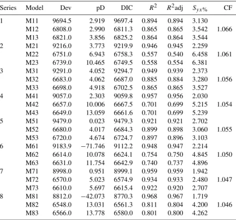
Indus-Table 3.Statistics of aboveground biomass (AGB) estimation models fit in a terra firme forest near Manaus, Amazonas, Brazil. See Table 2 for predictors and applied variance modeling approaches and Table A3 for the models’ parameters.
Series Model Dev pD DIC R2 R2adj Syx% CF
1 M11 9694.5 2.919 9697.4 0.894 0.894 3.130
M12 6808.0 2.990 6811.3 0.865 0.865 3.542 1.066
M13 6821.0 3.856 6825.2 0.864 0.864 3.544
2 M21 9216.0 3.773 9219.9 0.946 0.945 2.259
M22 6751.0 6.943 6758.3 0.557 0.540 6.458 1.061
M23 6739.0 10.465 6749.5 0.558 0.554 6.381
3 M31 9291.0 4.052 9294.7 0.949 0.939 2.373
M32 6683.0 4.062 6687.0 0.885 0.884 3.280 1.056
M33 6698.0 4.918 6702.5 0.865 0.865 3.527
4 M41 9057.0 2.303 9059.8 0.957 0.956 2.030
M42 6657.0 10.006 6667.5 0.701 0.699 5.215 1.054
M43 6649.0 13.059 6661.6 0.701 0.699 5.239
5 M51 9479.0 0.023 9479.3 0.921 0.921 2.702
M52 6680.0 4.017 6684.3 0.899 0.898 3.060 1.055
M53 6720.0 4.674 6724.7 0.897 0.896 3.103
6 M61 9183.9 −71.746 9112.2 0.948 0.947 2.214
M62 6614.0 10.078 6624.1 0.754 0.750 4.845 1.050
M63 6631.0 11.754 6642.9 0.740 0.737 4.896
7 M71 8998.0 0.951 8999.1 0.959 0.959 1.942
M72 6570.0 5.023 6574.9 0.934 0.933 2.480 1.047
M73 6610.0 5.697 6615.4 0.922 0.920 2.707
8 M81 8812.0 −42.073 8770.3 0.968 0.967 1.719
M82 6548.0 13.031 6561.3 0.811 0.804 4.200 1.046
M83 6566.0 13.778 6580.0 0.801 0.800 4.262
Parameters: models’ deviance (Dev), effective number of parameters (pD), deviance information criterion (DIC), coefficient of determination (R2), adjusted coefficient of determination (R2adj), relative standard error (Syx%)
and correction factor (CF) for models fit from ordinary least square with log-linear regressions.
tries, Inc, Boulder CO, USA). All codes used in this study were written by the authors.
3 Results
3.1 Individual tree biomass estimation model fits Although the NLS approach produced models with overall higher values of R2 andR2adj and lower values of Syx%,
the DIC values indicated that the MOV and the OLS ap-proaches produced the best models. The models M33 (DBH and WD as predictors) and M43 (DBH, SG and WD) were the two best fitting models across all tree individuals (high
R2 andR2adj and low Syx% and DIC values compared to
other models). These two models also produced more reli-able landscape predictions (see Sect. 3.2). The statistics for the goodness of fit for the 24 models are given in Table 3. For the models fit with OLS, which rely on log-transformed variables, the addition of other predictors together with DBH systematically decreased the CF values. This pattern suggests a reduction in the biases resulting from back transformation. As expected, the addition of other predictors to a model containing only DBH systematically increased the models’
parsimony, as indicated by the lower DIC values (Table 3). The inclusion of the SG assignment resulted in models with slightly lowerR2adj and higherSyx%compared to the same
model structure without SG.
We observed differences with respect to the parameters b and c among pioneer, mid- and late-successional species in most of the models that included the SG assignment (Ta-ble S3 and Fig. S1). The late-successional species tended to have higher intercepts and steeper slopes. Pioneer and mid-successional species had lower differences in intercepts but still strong differences in the slopes.
Evaluations of AGB predictions for individual trees from our two best models (as described in the Sect. 3.2) as well from the pantropical model (Chave et al., 2014) are presented in the Supplement of this study (Fig. S1). The models M33 and M43 had lower biases (overestimation of 0.6 and 3.5 %, respectively) than the tested pantropical model (underestima-tion of 30 %).
3.2 Landscape-level biomass predictions across scenarios
Figure 3.Predicted vs. observed aboveground biomass (AGB) along six forest scenarios composed of 100 1 ha plots. The line of equality (1:1 line) is shown as a red/straight line. Forest scenarios were designed to reflect landscape-level variations in floristic composition and size distribution of trees, typical of central Amazonian terra firme forests. Floristic composition and size-distribution scenarios followed the sampling scheme described in Sect. 2.4.2 (Fig. 2) of this study. Models’ predictors: diameter at breast height (DBH) (cm), species’ successional group (SG) (pioneers, mid- and late successional) and wood density (WD) (g cm−3). See Table 2 for the variance modeling approach of different equations. Note that models containing tree total height (H )as predictor were excluded here.
a predictor; Table 2) across the 100 1 ha plots assembled for each of our six forest scenarios (Figs. 3–5) as well as jointly for all of them (Fig. 6).
The “true” AGB in our 1 ha plots (from the summed mass of trees used to assemble the forest scenarios) varied from 198.1 to 314.3 (early- to late-successional scenarios) and 101.4 to 391.8 Mg ha−1 (small- to large-sized scenarios). The ability of the various biomass estimation models to pre-dict the “true” virtual biomass values generally reflected the goodness of fit of the models for predicting individual tree data (Table 3 and Figs. 3–6). The same pattern was observed when evaluating the tested pantropical model, which under-estimated both the AGB of individual trees (Fig. S1) and in all of our scenarios (Table S4 and Fig. S2).
While some models produced accurate and satisfactory predictions across all scenarios, others systematically under-or overestimated the observed AGB (Fig. 3 and Fig. S2). The agreement between models and observations was influenced not only by the different combinations of predictors but also by the different methods to model the variance. Interestingly, despite producing the best fits to the individual tree data, models fit with NLS produced the least reliable landscape-level predictions, with model M11 (only DBH as predictor) being the unique exception for the mid- and late-successional scenarios (Fig. 3).
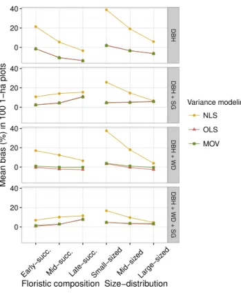
We observed systematic biases ranging from −14 % (underestimation) to 38.8 % (overestimation) in estimated landscape-level AGB (Fig. 4). The models fit with NLS tended to overestimate landscape-level AGB, with biases ranging from−3.6 up to 38.8 %, both extreme values from model series 1 (only DBH as predictor). Overall, the mod-els fit with NLS tended to capture changes in floristic com-position better than in tree size distribution. The tested pantropical model systematically underestimated landscape-level biomass, with a mean bias of−29.7 % (Table S4 and Fig. S2).
The models fit with the OLS and particularly with the MOV approaches were clearly more efficient at capturing the variation in floristic composition and size distribution of trees. Consequently, these models produced the most reliable landscape-level predictions within the scenarios (Fig. 3). As also indicated by the individual tree model fits, the MOV ap-proach produced more reliable AGB predictions, especially with model series 2 and 4.
0 20 40
0 20 40
0 20 40
0 20 40
DBH
DBH + SG
DBH + WD
DBH + WD + SG
Ear ly−succ.
Mid−succ.Late−succ.Small−siz ed
Mid−siz ed
Large−siz ed
Floristic composition Size−distribution
Mean bias (%) in 100 1−ha plots
Variance modeling
NLS
OLS
MOV
Figure 4.Profiles relating the bias of 12 aboveground tree biomass estimation models tested along six forest scenarios composed of 100 1 ha plots. Forest scenarios were designed to reflect landscape-level variations in floristic composition and size distribution of trees, typical of central Amazonian terra firme forests. Models’ predictors: diameter at breast height (DBH) (cm), species’ succes-sional group (SG) (pioneers, mid- and late successucces-sional) and wood density (WD) (g cm−3). Variance modeling approaches: nonlinear least square (NLS), ordinary least square with log-linear regression (OLS) and nonlinear with modeled variance (MOV). Note that mod-els containing tree total height (H) as predictor were excluded here.
with extreme values from model series 1 and 2, respectively (Fig. 4).
The reported systematic biases led to strong differences between the predicted and the observed AGB (Fig. 5). The models fit with NLS resulted in RMSE values ranging from 16.8 up to 125.8 Mg ha−1. For the models fit with OLS, the RMSE values ranged from 5.1 to 57.6 Mg ha−1. The MOV models had RMSE ranging from 5.5 to 58.7 Mg ha−1. The pantropical model’s predictions had a mean RMSE of 102.6 Mg ha−1(Table S4).
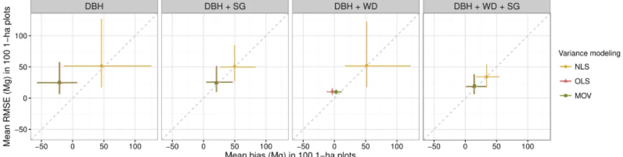
By combining the bias and RMSE values, we could ob-serve the overall models’ performance in predicting AGB across scenarios (Fig. 6). When challenged to predict biomass across all scenarios, the models fit with the MOV approach produced more reliable predictions (smaller range of biases and RMSE), except for model series 1 (only DBH as a predictor), for which the OLS approach performed bet-ter. Independently of applied predictors, the NLS approach had the highest mean and range of values for bias and RMSE.
0 25 50 75 100 125
0 25 50 75 100 125
0 25 50 75 100 125
0 25 50 75 100 125
DBH
DBH + SG
DBH + WD
DBH + WD + SG
Early −suc
c.
Mid−succ.Late−succ.Sm all−
size d
Mid− size
d
Larg e−si
zed
Floristic composition and size distribution
Mean RMSE
(Mg ha
−1
) in 100 1−ha plots
Variance modeling
NLS
OLS
MOV
Figure 5.Profiles relating the root-mean-square error of 12 above-ground tree biomass estimation models tested along six forest sce-narios composed of 100 1 ha plots. Forest scesce-narios were designed to reflect landscape-level variations in floristic composition and size distribution of trees, typical of central Amazonian terra firme forests. Models’ predictors: diameter at breast height (DBH) (cm), species’ successional group (SG) (pioneers, mid- and late succes-sional) and wood density (WD) (g cm−3). Variance modeling ap-proaches: nonlinear least square (NLS), ordinary least square with log-linear regression (OLS) and nonlinear with modeled variance (MOV). Note that models containing tree total height (H) as pre-dictor were excluded here.
As we expected, the addition of SG and WD improved the quality of the joint prediction. This was evidenced by the sys-tematic reduction of models’ bias and RMSE. Notably for the NLS approach, the inclusion of SG led to strong reduction of the bias and RMSE (Fig. 6). Interestingly, for this approach the addition of WD alone did not improve the estimations accuracy.
4 Discussion
DBH DBH + SG DBH + WD DBH + WD + SG
−50 0 50 100
−50 0 50 100 −50 0 50 100 −50 0 50 100 −50 0 50 100
Mean bias (Mg) in 100 1−ha plots
Mean RMSE (Mg) in 100 1−ha plots
Variance modeling NLS OLS MOV
Figure 6.Overall performance of 12 aboveground tree estimation models along six forest scenarios composed of 100 1 ha plots. Forest sce-narios were designed to reflect landscape-level variations in floristic composition and size distribution of trees, typical of central Amazonian terra firme forests. Models are rated by the absolute mean bias and root-mean-square error (RMSE), both in Mg. Solid points and bars rep-resent absolute mean and range values, respectively. Models’ predictors: diameter at breast height (DBH) (cm), species’ successional group (SG) (pioneers, mid- and late successional) and wood density (WD) (g cm−3). Variance modeling approaches: nonlinear least square (NLS), ordinary least square with log-linear regression (OLS) and nonlinear with modeled variance (MOV). Note that models containing tree total height (H) as predictor were excluded here.
of these two predictors to the basic DBH model yielded a more consistent model than addingH (Table S3). This pat-tern was true for all the three variance modeling approaches and supports having the species’ identification (i.e., further assignment into SGs) and/or coherent wood density values, which is crucial when aiming for precise tree AGB predic-tions. Since old-growth forests comprise a mosaic of differ-ent successional stages, with trees of various architectures and sorted into different forest layers/strata, these variables are especially important when aiming for reliable AGB pre-dictions at the landscape level (see Sect. 4.2).
Although the NLS approach fits our data set better (higher
R2adj and lowerSyx%), the assumption of a constant
vari-ance violates the natural heteroscedasticity of allometric data sets. With the log transformation of the OLS approach, ho-moscedasticity is reached but in a way that does not exactly reflect how variance actually changes. As previously reported for Amazon terra firme forests (Chambers et al., 2001; Lima et al., 2012), models fit with the OLS approach tend to over-estimate the biomass of large-sized trees.
Indeed, the best models are obtained using the MOV and OLS approaches, in which we explicitly modeled variance depending on the main predictor (DBH). This explains why the models fit with these approaches produced more reliable (i.e., smaller differences between predictions and observa-tions) AGB estimates as compared to those fit with the NLS approach. The NLS approach is still frequently found in the literature (Sileshi, 2014), despite the fact that assuming con-stant variance is not an appropriate choice for allometric data sets. We included the latter approach mainly for illustrative purposes.
Despite the highly heterogeneous nature of our data set (Table 1 and Table S1), DBH alone still captures a large frac-tion of the variafrac-tion in AGB. This could be confirmed by lower Syx% values within model series 1 in comparison to
the other model series (Table 2). This result illustrates that
ignoring selection criteria that capture a model’s capacity to make predictions for new predictor combinations (e.g., dif-ferent region or successional stage), such as the DIC or our landscape-level evaluation (see Sect. 4.2), can lead to the wrong choice. The basic models containing only DBH had a higher DIC in comparison to other model series and con-sequently did poorly in predicting the AGB of our different landscape scenarios (Fig. 6).
Our data set contains a large number of species, which allowed for the maximum expression of architectural at-tributes. In comparison to species-specific biomass estima-tion models (Nelson et al., 1999) or models fit from data collected in undisturbed and homogenous forests (Higuchi et al., 1998; Lima et al., 2012), we expected the addition of predictors reflecting architectural and anatomical variation to improve model parsimony. This pattern was observed when adding both SG and WD (Fig. 6 and Table S3).
The differences related to the parametersbandcwe found among our successional groups highlighted the importance of using SG as a predictor of the architectural attributes that influence allometry, especially in disturbed or secondary forests where WD is not available (Table S3). In the mod-els containing SG, the significant variation of the parame-tersb and c between pioneers, mid- and late-successional species highlights the importance of architectural attributes on defining allometries (Nelson et al., 1999). Often, these differences were neglected in previous studies that dealt with heterogeneous data sets and aimed at parameterizing global/pantropical biomass estimation models.
we attribute part of this pattern to strong differences in forest structure and tree allometry/architecture between our central Amazon data set and that used to parameterize the pantropi-cal model from Chave et al. (2014). Although the DBH and
H range of the trees used in our study is well represented by the pantropical data set, the two data sets vary strongly with respect to the DBH and H distribution of trees (Fig. S3). Our data set clearly has a much higher density of small-sized trees and a much lower density of large-small-sized trees. The pantropical data set comprises ca. 8 % (n=329) of trees with DBH≥60 cm and meanH of 39.3 m (and even a tree with 212 cm DBH and another one with 70.7 mH ). Interestingly, none of these 329 large-sized trees were found in terra firme forests in the region of Manaus. Note that the largest tree in our data set has 85 cm DBH and 33 mH (Table 1 and Ta-ble S1) and, as previously reported, trees with DBH≥60 cm account for less than 17 % of the total AGB in central Ama-zonian terra firme forests (Vieira et al., 2004). Thus the struc-ture and biomass of these central Amazonian forests is not well predicted from the “improved” pantropical biomass es-timation model from Chave et al., 2014.
Observed differences on the relationship between predic-tor variables (DBH and WD) and AGB of trees from our data set and that used in the pantropical model highlight part of the variation in tree allometry and architecture that was not represented in the pantropical data set (Fig. S4). As for the differences in forest structure, these differences in tree al-lometry and architecture reflect typical differences in species composition among successional stages (Clark and Clark, 1992; Denslow, 1980; Marra et al., 2014). By including our two secondary forests, we added a greater proportion of al-lometric variation in our models compared to the Chave et al. (2014) data set (Fig. S5). Our results indicate that neglect-ing variations in tree allometry and architecture related to floristic composition can lead to strong bias when predicting individual tree AGB, especially when complex old-growth and secondary forests (Asner, 2013; Chambers et al., 2013; Norden et al., 2015) are not accounted for in the model pa-rameterization.
4.2 Landscape-level biomass predictions across scenarios
The different combinations of floristic composition and structure (i.e., tree density and basal area) used in our virtual approach reflected forest changes along succession (Cham-bers et al., 2009; Marra et al., 2014; Norden et al., 2015), in-cluding realistic variations in AGB reported for central Ama-zon stands differing in successional stage (from early succes-sional to old growth) (Carvalho Jr. et al., 1995; Higuchi et al., 2004; Lima et al., 2007). When taking into account the accuracy of landscape-level predictions across scenarios, the best models were those fit by using the MOV and the OLS approaches. From the MOV approach, the models M33, M43
and M23 were the first, second and third best models, respec-tively (Fig. 6).
Modeling the variance properly as in the MOV approach is particularly important when both small and large trees – at the respective endpoints of the size predictors DBH and
H – are to be estimated precisely. Assuming homoscedas-tic variance in allometric data gives a stronger weight to the information of large trees (which have large residuals) and reduces the “strength” of the small trees (with small residu-als) on the estimation of the parameters. This almost invari-ably leads to models that overestimate the biomass of small trees (i.e., large trees pulling the “line” upwards). This effect can be clearly seen in Fig. 4 where the NLS models dramat-ically overestimated the biomass, particularly in the small-sized and the early-successional scenario. The OLS approach tends to produce the opposite effect. The log transformation shrinks the size of the residuals of the large-sized trees and inflates it for the small-sized trees. The influence of positive residuals or large-sized trees that often have a strong lever is reduced, and the lever of very small trees is increased. This may (although not as extremely as in the NLS case) lead to an underestimation of the biomass of big trees. A slight ten-dency of this effect is also visible in Fig. 4 when the OLS and MOV models are compared in the model series 2 and 3. The model evaluation with our virtual forests thus clearly illustrates that a balanced modeling of the variance, i.e., giv-ing the small and large trees equal weight, is very important when (1) the design matrices are very heterogeneous or un-balanced with respect to size and when (2) predictions are made at landscape level across stands that vary in the mean size/shape of trees.
Models containing only size predictors (such as DBH) are particularly sensitive to this problem. Including SG and WD as predictors captured part of the interspecific variation in architecture and anatomy and partly alleviated the above-mentioned problems of the NLS and OLS models. Thus, al-though a simple allometric model (e.g., AGB∼b1DBHb2)
can accurately describe the DBH : AGB relationship at the individual level (Table 3 and Table S3), our results demon-strate that reliable estimates of biomass in heterogeneous landscapes (i.e., mixtures of successional stages and tree sizes) requires correct modeling of the size-related variance (Sileshi, 2014; Todeschini et al., 2004) and including suitable predictors of species-specific attributes reflecting ecological, architectural and anatomical variation.
and possibly be ignored (Gregoire et al., 2016; McRoberts and Westfall, 2014). However, since we constructed the for-est scenarios with trees from our data set, this is an “in-ternal evaluation” and not a test of model behavior in the face of new predictor combinations. Furthermore, we used DIC as parsimony-based model selection criterion, which was designed to exactly approximate this capacity and typ-ically yields similar results as cross-validation (Wirth et al., 2004). The DIC is therefore particularly important for judg-ing the quality of the model, especially for application in other regions or for other species. Unlike the virtual forest approach, where the DBH + WD with modeled variance (M33) appeared to be the best model (lowest bias and RMSE at the same time) (Fig. 6), the DIC invariably requires the full model complexity irrespective of whetherHis considered or not (Table 3).
As reported in other studies (Alvarez et al., 2012; Lima et al., 2012; Ngomanda et al., 2014; Nogueira Jr. et al., 2014), using the pantropical biomass estimation model by Chave et al. (2014) for landscape-level predictions led to strong bi-ases in the case of our central Amazonian forest scenarios. Thus, our recommendation is not to assume that their model is equally applicable across all tropical forests, especially for secondary or hyperdiverse tropical forests. In this context, we alert researches and managers about the importance of applying local or regional generic models when estimating biomass and the importance of species composition informa-tion in plot studies.
4.3 Suitability of the chosen predictors for practical application
As we have seen, predicting biomass correctly at the land-scape level and in particular improving performance at the fringes or outside the predictor space requires the inclusion of predictors related to species architecture (DBH in com-bination withH (when available), WD and/or SG). Knowl-edge of these last two variables depends on the identification of species, further assignment into successional groups and measurement or compilation of species-specific WD values. For the purposes of our study, these variables were success-fully addressed.
However, we understand that reliable biomass estimation models also require variables that can be easily and confi-dently acquired or measured. As we discuss below, this is not the case for the species identification,H and, consequently, in many cases for WD and SG.
The tree species diversity in the Amazon is high (de Oliveira and Mori, 1999; ter Steege et al., 2013). Species identification requires extensive field work (i.e., collection of botanical samples) and joint effort of parabotanists, botanists and taxonomists. In many cases, this task might pose a major problem.
For WD, values can vary widely not only between species (Chave et al., 2006) – which we exploit in our modeling
ap-proach – but also between different sites/regions (Muller-Landau, 2004), within individuals of the same species or even in an individual tree (density varying along the tree bole) (Higuchi et al., 1998; Nogueira et al., 2005). Ide-ally, WD measures should be carried out in situ follow-ing a method that allows for samplfollow-ing both heart- and sap-wood. Measuring WD from nonrepresentative samples and applying measures from studies in which samples were oven dried at different temperatures can produce compli-cation. At temperatures below 100◦C, the wood bound water content cannot be removed (Williamson and Wie-mann, 2010). This requires improvement of available meth-ods and tools (e.g., resistography, X-ray, ultrasonic tomog-raphy, near-infrared spectroscopy, acoustic/ultrasonic wave propagation and high-frequency densitometry) (Isik and Li, 2003; Lin et al., 2008; Schinker et al., 2003) that in the future may allow the measurement of WD in live trees from hyper-diverse tropical forests (thousands of species). However, the acquisition of WD data is still expensive and is not easily conducted simultaneously with forest inventories.
In the Amazon, information on WD is not available at the species level for most regions, and the available WD data have been acquired using a wide range of methods. Thus, the compilation of WD data from different sources without filtering criteria may introduce an unpredictable source of er-ror. As a result, researchers and managers need to establish robust criteria and test whether including WD information compiled from the available literature can really increase the quality of biomass predictions (as shown in our study). These limitations become critical when adjusting biomass estima-tion models both from small or even large/combined data sets collected without a plot-based harvest method that allows for a landscape-level evaluation of models derived using indi-vidual trees (Carvalho Jr. et al., 1995; Higuchi et al., 1998; Lima et al., 2012; da Silva, 2007). One important result of our study is that correct assignment of species into successional groups can satisfactorily replace the use of WD despite the fact that WD and SG were not trivially correlated (Table 2).
Most of the available biomass estimation models include
Has a predictor. Indeed, we expected the inclusion ofHto substantially improve our individual tree fits and landscape-level predictions. Although H is a powerful predictor of AGB, because together with DBH it defines the slender-ness of trees and also indicates the lifetime light availabil-ity (suppressed trees with typically short crowns have a high
our (Table 2) and other data sets (Sileshi, 2014), the high collinearity between DBH andHcan distort coefficient val-ues, inflate standard errors and lead to unreliable estimates. The increased availability of new tools such as Lidar can im-prove the resolution of data on tree height and thus biomass (Marvin et al., 2014; Sawada et al., 2015), but currently the areas where such data are available are limited. The cali-bration of remote-sensing-based biomass models for diverse tropical forest still relies on the degree of uncertainty associ-ated to plot-level AGB estimates (Chen et al., 2015).
Despite uncertainties associated with global estimates of carbon stocks, tropical forests store ca. 25 % of the terrestrial carbon (Bonan, 2008; Saatchi et al., 2011) and provide re-sources (e.g., food, fuel, timber and water) essential for hu-mankind (Trumbore et al., 2015). Nonetheless, old-growth tropical forests are rapidly changing and degrading due to the intensification of human activities, gradual climate change and extreme weather events (FAO, 2010; IPCC, 2014). The Reducing Emissions from Deforestation and Forest Degra-dation (REDD+)program from the United Nations Frame-work Convention on Climate Change (UNFCCC) establishes rewards for actions that mitigate carbon emission through prevention of forest loss and degradation. For countries with large forest cover (e.g., Brazil and other Amazonian coun-tries), such programs emerge as an economical alternative to historically more lucrative land uses resulting in forest degra-dation or suppression. However, we showed that reliable es-timates of forest biomass are complex to obtain and prone to large uncertainty. Reliable predictions of biomass/carbon stocks over large regions of structurally complex and hy-perdiverse tropical forests such as the Amazon still depend on the collection of plot-based allometric data and forest in-ventories including information on species composition, tree height and wood density, which are often unavailable or esti-mated imprecisely in most regions.
Natural and anthropogenic tropical secondary forests are widely distributed and account for ca. 50 % of the global forest cover (FAO, 2010). Although highly productive and resilient (Poorter et al., 2016), Neotropical forests can take unpredictable successional trajectories (Norden et al., 2015). During forest succession, once floristic composition changes and structural gradients increase, allometry becomes more complex and reliable landscape-level biomass esti-mates may require models that include predictors approxi-mating species-specific architecture and anatomy. Extra care should be taken when using biomass estimation models to assess biomass dynamics (e.g., biomass recovery after distur-bances). Earlier stages of recovery can have a higher propor-tion of small trees from pioneers species, which have lower wood density (Chambers et al., 2009; Marra et al., 2014; Sal-darriaga et al., 1998) and a particular type of architecture (Hallé et al., 1978; Swaine and Whitmore, 1988).
We recommend the use of the best models fit in this study when aiming for reliable landscape AGB estimations for cen-tral Amazonian terra firme forests, especially those under
complex disturbance regimes and for which specific/local models are not available. When data on species composition and wood density are available or could be accurately com-piled from the literature, we encourage the use of the model M33 or M23 (MOV approach). In case the MOV approach cannot be applied for model parameterization (i.e. technical or computational restrictions), the OLS is presumably more appropriate and efficient than the NLS.
The Supplement related to this article is available online at doi:10.5194/bg-13-1553-2016-supplement.
Acknowledgements. This study has been possible thanks to the extensive fieldwork carried by members of the Laboratório de Manejo Florestal (LMF) from the Instituto Nacional de Pesquisas da Amazônia (INPA). We gratefully acknowledge: Antônio F. da Silva, Armando N. Colares, Bertrán A. da Silva (in memoriam), Geraldo A. da Mota, Geraldo E. da Silva, Francinil-ton R. de Araújo, Francisco H. M. dos Santos, Francisco Q. Reis, José M. de Souza, José M. B. da Paz, José M. G. Quintanilha Junior, Manoel F. J. de Souza, Manoel N. Taveira, Paulo J. Q. de Lac-erda (in memoriam), Pedro L. de Figueiredo (in memoriam), Romeu D. de Paiva, Sebastião M. do Nascimento, Sérgio L. Leite, Valdecira M. J. Azevedo and Wanderley de L. Reis. This study was financed by the Brazilian Council for Scientific and Techno-logical Development (CNPq) within the projects Piculus, INCT Madeiras da Amazônia and Succession After Windthrows (SAWI) (Chamada Universal MCTI/No 14/2012, Proc. 473357/2012-7), and supported by the Max Planck Institute for Biogeochemistry within the Tree Assimilation and Carbon Allocation Physiology Experiment (TACAPE). Robinson I. Negrón-Juárez was supported by the Office of Science, Office of Biological and Environmental Research, of the US Department of Energy under contract no. DE-AC02-05CH11231 as part of Next-Generation Ecosystems Experiments (NGEE Tropics) and the Regional and Global Climate Modeling (RGCM) Program.
The article processing charges for this open-access publication were covered by the Max Planck Society.
Edited by: J. Schöngart
References
Alvarez, E., Duque, A., Saldarriaga, J., Cabrera, K., de las Salas, G., del Valle, I., Lema, A., Moreno, F., Orrego, S., and Rodríguez, L.: Tree above-ground biomass allometries for carbon stocks es-timation in the natural forests of Colombia, Forest Ecol. Manag., 267, 297–308, 2012.
Asner, G. P.: Geography of forest disturbance, P. Natl. Acad. Sci. USA, 110, 3711–3712, 2013.
Banin, L., Feldpausch, T. R., Phillips, O. L., Baker, T. R., Lloyd, J., Affum-Baffoe, K., Arets, E. J. M. M., Berry, N. J., Bradford, M., Brienen, R. J. W., Davies, S., Drescher, M., Higuchi, N., Hilbert, D. W., Hladik, A., Iida, Y., Salim, K. A., Kassim, A. R., King, D. A., Lopez-Gonzalez, G., Metcalfe, D., Nilus, R., Peh, K. S. H., Reitsma, J. M., Sonké, B., Taedoumg, H., Tan, S., White, L., Wöll, H., and Lewis, S. L.: What controls tropical forest architec-ture? Testing environmental, structural and floristic drivers, Glob. Ecol. Biogeogr., 21, 1179–1190, 2012.
Bolker, B. M.: Ecological Models and Data in R, Princeton Univer-sity Press, New Jersey, 2008.
Bolker, B. M., Gardner, B., Maunder, M., Berg, C. W., Brooks, M., Comita, L., Crone, E., Cubaynes, S., Davies, T., de Valpine, P., Ford, J., Gimenez, O., Kéry, M., Kim, E. J., Lennert-Cody, C., Magnusson, A., Martell, S., Nash, J., Nielsen, A., Regetz, J., Skaug, H., and Zipkin, E.: Strategies for fitting nonlinear eco-logical models in R, AD Model Builder, and BUGS, Methods Ecol. Evol., 4, 501–512, 2013.
Bonan, G. B.: Forests and climate change: forcings, feedbacks, and the climate benefits of forests, Science, 320, 1444–1449, doi:10.1126/science.1155121, 2008.
Bowman, D. M. J. S., Brienen, R. J. W., Gloor, E., Phillips, O. L., and Prior, L. D.: Detecting trends in tree growth: Not so simple, Trends Plant Sci., 18, 11–17, 2013.
Braga, P. I. S.: Subdivisão fitogeográfica, tipos de vegetação, con-servação e inventário florístico da floresta amazônica, Acta Amaz., 9, 53–80, 1979.
Brooks, S. P. and Gelman, A.: General Methods for Monitoring Convergence of Iterative Simulations, J. Comput. Graph. Stat., 7, 434–455, 1998.
Brooks, S. P. and Roberts, G. O.: Convergence assessment tech-niques for Markov chain Monte Carlo, Stat. Comput., 8, 319– 335, 1998.
Brown, S., Gillespie, A. J. R., and Lugo, A. E.: Biomass estimation methods for tropical forests with applications to forest inventory data, Forest Sci., 35, 881–902, 1989.
Carvalho Jr., J. A., Santos, J. M., Santos, J. C., Leitão, M. M., and Higuchi, N.: A tropical rainforest clearing experiment by biomass burning in the Manaus region, Atmos. Environ., 29, 2301–2309, 1995.
Chambers, J., Higuchi, N., Teixeira, L., Santos, J. dos, Laurance, S., and Trumbore, S.: Response of tree biomass and wood litter to disturbance in a Central Amazon forest, Oecologia, 141, 596– 611, 2004.
Chambers, J. Q., dos Santos, J., Ribeiro, R. J., and Higuchi, N.: Tree damage, allometric relationships, and above-ground net primary production in central Amazon forest, Forest Ecol. Manag., 152, 73–84, 2001.
Chambers, J. Q., Robertson, A. L., Carneiro, V. M. C., Lima, A. J. N., Smith, M. L., Plourde, L. C., and Higuchi, N.: Hyperspectral remote detection of niche partitioning among canopy trees driven by blowdown gap disturbances in the Central Amazon, Oecolo-gia, 160, 107–117, 2009.
Chambers, J. Q., Negron-Juarez, R. I., Marra, D. M., Di Vittorio, A., Tews, J., Roberts, D., Ribeiro, G. H. P. M., Trumbore, S. E., and Higuchi, N.: The steady-state mosaic of disturbance and
suc-cession across an old-growth Central Amazon forest landscape, P. Natl. Acad. Sci. USA, 110, 3949–3954, 2013.
Chave, J., Andalo, C., Brown, S., Cairns, M. A., Chambers, J. Q., Eamus, D., Fölster, H., Fromard, F., Higuchi, N., Kira, T., Les-cure, J. P., Nelson, B. W., Ogawa, H., Puig, H., Riéra, B., and Yamakura, T.: Tree allometry and improved estimation of carbon stocks and balance in tropical forests, Oecologia, 145, 87–99, 2005.
Chave, J., Muller-Landau, H. C., Baker, T. R., Easdale, T. A., Hans Steege, T. E. R., and Webb, C. O.: Regional and phylogenetic variation of wood density across 2456 neotropical tree species, Ecol. Appl., 16, 2356–2367, 2006.
Chave, J., Coomes, D., Jansen, S., Lewis, S. L., Swenson, N. G., and Zanne, A. E.: Towards a worldwide wood economics spectrum, Ecol. Lett., 12, 351–366, 2009.
Chave, J., Réjou-Méchain, M., Búrquez, A., Chidumayo, E., Col-gan, M. S., Delitti, W. B. C., Duque, A., Eid, T., Fearnside, P. M., Goodman, R. C., Henry, M., Martínez-Yrízar, A., Mu-gasha, W., Muller-Landau, H. C., Mencuccini, M., Nelson, B. W., Ngomanda, A., Nogueira, E. M., Ortiz-Malavassi, E., Pélissier, R., Ploton, P., Ryan, C. M., Saldarriaga, J. G., and Vieilledent, G.: Improved allometric models to estimate the aboveground biomass of tropical trees, Glob. Chang. Biol., 20, 3177–3190, 2014.
Chen, Q., Vaglio Laurin, G., and Valentini, R.: Uncertainty of re-motely sensed aboveground biomass over an African tropical for-est: Propagating errors from trees to plots to pixels, Remote Sens. Environ., 160, 134–143, doi:10.1016/j.rse.2015.01.009, 2015. Clark, D. A. and Clark, D. B.: Life history diversity of canopy and
emergent trees in a neotropical rain forest, Ecol. Monogr., 62, 315–344, 1992.
Clark, D. B. and Kellner, J. R.: Tropical forest biomass estimation and the fallacy of misplaced concreteness, J. Veg. Sci., 23, 1191– 1196, 2012.
da Silva, R.: Alometria, estoque e dinânica da biomassa de flo-restas primárias e secundárias na região de Manaus (AM), PhD Thesis, Universidade Federal do Amazonas, Brazil, available at: https://www.inpa.gov.br/arquivos/Tese_Biomassa_Roseana_ Silva.pdf (last access: 5 March 2015), 2007.
da Silva, R. P., dos Santos, J., Tribuzy, E. S., Chambers, J. Q., Naka-mura, S., and Higuchi, N.: Diameter increment and growth pat-terns for individual tree growing in Central Amazon, Brazil, For-est Ecol. Manag., 166, 295–301, 2002.
da Silva, R. P., Nakamura, S., Azevedo, C. de, Chambers, J., Rocha, R. de M., Pinto, C., dos Santos, J., and Higuchi, N.: Use of metal-lic dendrometers for individual diameter growth patterns of trees at Cuieiras river basin, Acta Amaz., 33, 67–84, 2003.
Denslow, J. S.: Patterns of plant species diversity during succession under different disturbance regimes, Oecologia, 46, 18–21, 1980. de Oliveira, A. A. and Mori, S. A.: A central Amazonian terra firme forest. I. High tree species richness on poor soils, Biodivers. Con-serv., 8, 1219–1244, 1999.
dos Santos, J.: Análise de modelos de regressão para estimar a fit-omassa da floresta tropical úmida de terra-firme da Amazônia Brasileira, Ph.D. Thesis, Universidade Federal de Viçosa, Minas-Gerais, Brazil, 1996.