ACPD
15, 26997–27039, 2015Sky imager based solar irradiance
analysis and forecasts
T. Schmidt et al.
Title Page
Abstract Introduction
Conclusions References
Tables Figures
◭ ◮
◭ ◮
Back Close
Full Screen / Esc
Printer-friendly Version Interactive Discussion
Discussion
P
a
per
|
Discussion
P
a
per
|
Discussion
P
a
per
|
Discussion
P
a
per
|
Atmos. Chem. Phys. Discuss., 15, 26997–27039, 2015 www.atmos-chem-phys-discuss.net/15/26997/2015/ doi:10.5194/acpd-15-26997-2015
© Author(s) 2015. CC Attribution 3.0 License.
This discussion paper is/has been under review for the journal Atmospheric Chemistry and Physics (ACP). Please refer to the corresponding final paper in ACP if available.
Evaluating the spatio-temporal
performance of sky imager based solar
irradiance analysis and forecasts
T. Schmidt, J. Kalisch, E. Lorenz, and D. Heinemann
Department of Energy and Semiconductor Research, Carl von Ossietzky University Oldenburg, Oldenburg, Germany
Received: 27 August 2015 – Accepted: 4 September 2015 – Published: 7 October 2015 Correspondence to: T. Schmidt (t.schmidt@uni-oldenburg.de)
ACPD
15, 26997–27039, 2015Sky imager based solar irradiance
analysis and forecasts
T. Schmidt et al.
Title Page
Abstract Introduction
Conclusions References
Tables Figures
◭ ◮
◭ ◮
Back Close
Full Screen / Esc
Printer-friendly Version Interactive Discussion
Discussion
P
a
per
|
Discussion
P
a
per
|
Discussion
P
a
per
|
Discussion
P
a
per
|
Abstract
Clouds are the dominant source of variability in surface solar radiation and uncertainty in its prediction. However, the increasing share of solar energy in the world-wide electric power supply increases the need for accurate solar radiation forecasts.
In this work, we present results of a shortest-term global horizontal irradiance (GHI)
5
forecast experiment based on hemispheric sky images. A two month dataset with im-ages from one sky imager and high resolutive GHI measurements from 99 pyranome-ters distributed over 10 km by 12 km is used for validation. We developed a multi-step model and processed GHI forecasts up to 25 min with an update interval of 15 s. A cloud type classification is used to separate the time series in different cloud
scenar-10
ios.
Overall, the sky imager based forecasts do not outperform the reference persis-tence forecasts. Nevertheless, we find that analysis and forecast performance depend strongly on the predominant cloud conditions. Especially convective type clouds lead to high temporal and spatial GHI variability. For cumulus cloud conditions, the analysis
15
error is found to be lower than that introduced by a single pyranometer if it is used representatively for the whole area in distances from the camera larger than 1–2 km. Moreover, forecast skill is much higher for these conditions compared to overcast or clear sky situations causing low GHI variability which is easier to predict by persis-tence. In order to generalize the cloud-induced forecast error, we identify a variability
20
threshold indicating conditions with positive forecast skill.
1 Introduction
As a result of world-wide growing photovoltaic electricity production, the energy sector is facing new challenges. One major issue is solar variability (Sayeef et al., 2012), on short timescales mainly caused by changes in cloud cover. With an increased share
25
ACPD
15, 26997–27039, 2015Sky imager based solar irradiance
analysis and forecasts
T. Schmidt et al.
Title Page
Abstract Introduction
Conclusions References
Tables Figures
◭ ◮
◭ ◮
Back Close
Full Screen / Esc
Printer-friendly Version Interactive Discussion
Discussion
P
a
per
|
Discussion
P
a
per
|
Discussion
P
a
per
|
Discussion
P
a
per
|
getting more and more challenging for power plant and grid operators. Consequently, flexibility options, like demand-side management, backup capacities, inverter control, storages and strengthening of the grid are in the focus of research. In order to control and manage the flexibility options the expected solar power production is an important information. Although the large variety of cloud characteristics (opacity, motion, height,
5
spatial distribution) make these cloud-induced fluctuations difficult to predict, solar ir-radiance forecasting techniques have been successfully developed (a comprehensive overview is given in Inman et al., 2013, and Lorenz and Heinemann, 2012). The spec-trum comprises numerical weather models (NWP) (Perez et al., 2013), satellite-based forecasts using cloud motion vectors (Kühnert et al., 2013; Lorenz et al., 2004;
Ham-10
mer et al., 1999), statistical methods based on machine learning (Wolff et al., 2013) and time series analysis (Reikard, 2009) predominantly developed for intra-day and day ahead forecasts. For very short term forecasts with horizons of up to 30 min, both NWP and satellite image-based models lack spatial and temporal resolution regarding cloud-induced small-scale variability (Inman et al., 2013).
15
Filling this gap of local high resolutive and very short-term forecasts research has been spent recently on the use of ground-based (whole/all/total) sky imagers. Sky im-agers have been used for years for monitoring cloud cover characteristics (Pfister et al., 2003; Long et al., 2006; Cazorla et al., 2008) and aerosol properties (Olmo et al., 2008; Cazorla, 2010).
20
The development of solar radiation forecast methods based on sky images has been intensified in recent years (Chu et al., 2015; West et al., 2014; Quesada-Ruiz et al., 2014; Chu et al., 2013; Fu and Cheng, 2013; Yang et al., 2014; Bernecker et al., 2014; Chow et al., 2011; Marquez and Coimbra, 2013).
By analysing distribution, movement and optical properties of clouds the incoming
25
ACPD
15, 26997–27039, 2015Sky imager based solar irradiance
analysis and forecasts
T. Schmidt et al.
Title Page
Abstract Introduction
Conclusions References
Tables Figures
◭ ◮
◭ ◮
Back Close
Full Screen / Esc
Printer-friendly Version Interactive Discussion
Discussion
P
a
per
|
Discussion
P
a
per
|
Discussion
P
a
per
|
Discussion
P
a
per
|
cloud motion (speed and direction), respectively. Two types of forecast experiments are reported in recent work. Point forecasts only predict the occlusion of the sun with clouds and therefore can only process forecasts for the place of the camera (e.g. West et al., 2014). Area forecasts, on the other hand, incorporate cloud base height in order to calculate the location of clouds and shadows on the ground (e.g. Yang et al., 2014).
5
This work presents results of short-term area forecast experiments. We developed and applied a multi-step model on a large dataset of sky images and processed fore-casts up to 25 min ahead for 99 locations distributed in the surrounding area. GHI measurements at these locations are used for evaluating the forecast performance. This work focuses on the investigation of the performance under different cloud
condi-10
tions. A cloud classification scheme is used to categorize the dataset in seven different cloud conditions. This differentiation is helpful in the comparison with reference models like persistence which are almost perfect for short forecast horizons and low variability in cloud cover. The spatial distribution of pyranometers is used to identify differences in performance for locations distant from the camera. This analysis is helpful for
inves-15
tigating the usefulness of sky imager based irradiance field analysis instead of using several expensive pyranometers. As our cloud detection scheme only provides two bi-nary states (sky/cloud) and no cloud transmissivity information, the irradiance retrieval for GHI has weaknesses in case of deviations from this simplification. Therefore, we also evaluate binary forecasts, in order to identify the contribution to the overall forecast
20
error caused by the irradiance retrieval.
The used dataset is introduced in Sect. 2. Section 3 presents details of the devel-oped sky imager based forecast model and the concept of evaluation. Results and Discussion are given in Sect. 4 and Conclusions in Sect. 5.
2 Experimental setup and database
25
ACPD
15, 26997–27039, 2015Sky imager based solar irradiance
analysis and forecasts
T. Schmidt et al.
Title Page
Abstract Introduction
Conclusions References
Tables Figures
◭ ◮
◭ ◮
Back Close
Full Screen / Esc
Printer-friendly Version Interactive Discussion
Discussion
P
a
per
|
Discussion
P
a
per
|
Discussion
P
a
per
|
Discussion
P
a
per
|
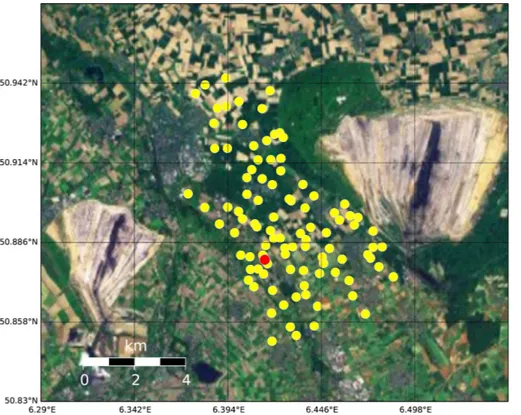
(HD(CP)2) measurement campaign HOPE in 2013. For this work, data from a network of 99 irradiance sensors, one ceilometer and one sky imager were used (Fig. 1). The following subsections give a short description of the used datasets. Here, measure-ments from 1 April to 31 May were used. The measurement site is located in Jülich, Germany. The area is rather flat and surrounded by two large lignite open-cast minings
5
(Fig. 1).
2.1 Sky imager
A sky imager developed at the GEOMAR Helmholtz Centre for Ocean Research (Kalisch and Macke, 2008) was used for continuous sky observations. The imager was part of the LACROS supersite within the HOPE measurement campaign, see
Mad-10
havan et al. (2015) for the location and details. The digital CCD camera by Canon equipped with a fisheye lens by Raynox realized a field of view of 183◦. The hemi-spheric sky images with 2592 pixel×1744 pixel resolution were sampled at a rate of
15 s.
2.2 Irradiance sensor network 15
A irradiance measurement network with 99 pyranometer stations was set up around Jülich, Germany on an area of 10 km×12 km. Each station was equipped with a EKO
ML-020VM photodiode pyranometer. The 10-bit data logging system was synchronized with the GPS time. The irradiance was measured with 10 Hz resolution and was aver-aged to 1 Hz. The maintenance as well as cleanliness and tilt control were performed
20
on a weekly basis.
ACPD
15, 26997–27039, 2015Sky imager based solar irradiance
analysis and forecasts
T. Schmidt et al.
Title Page
Abstract Introduction
Conclusions References
Tables Figures
◭ ◮
◭ ◮
Back Close
Full Screen / Esc
Printer-friendly Version Interactive Discussion
Discussion
P
a
per
|
Discussion
P
a
per
|
Discussion
P
a
per
|
Discussion
P
a
per
|
2.3 Additional data
Processing sky images for solar irradiance area forecasts need further information about cloud base height and sun position for ray tracing and following cloud shadow mapping. Clear sky irradiance information is necessary for reference cloud-free sky conditions and irradiance retrieval.
5
Information about cloud base height is retrieved from a Jenoptik CHM15k-x ceilome-ter, that was located next to the sky imager. Ceilometers are recognized by the WMO as the most accurate, reliable and efficient means of measuring cloud base from the ground when compared with alternative equipment (World Meteorological Organiza-tion, 2008). One measurement was done every 20 s. As a ceilometer provides only
10
point measurements, the median of the last 30 measurements was used in order to smooth the signal. Although multi-layer cloud height information is available, only lower level cloud height was used, because the used sky imager algorithm does not yet sup-port multilayer clouds. Clear sky irradiance is estimated with the clear sky model of Dumortier (Fontoynont et al., 1998) and turbidity values according to Bourges (1992)
15
and Dumortier (1998). The solar zenith and azimuth angle are calculated with the solar geometry2 (SG2) algorithm (Blanc and Wald, 2011).
3 Methods
In order to determine and predict the surface patterns of global horizontal irradiance distribution from sky images, several preprocessing steps on the image have to be
20
ACPD
15, 26997–27039, 2015Sky imager based solar irradiance
analysis and forecasts
T. Schmidt et al.
Title Page
Abstract Introduction
Conclusions References
Tables Figures
◭ ◮
◭ ◮
Back Close
Full Screen / Esc
Printer-friendly Version Interactive Discussion
Discussion
P
a
per
|
Discussion
P
a
per
|
Discussion
P
a
per
|
Discussion
P
a
per
|
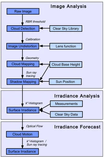
3.1 Image analysis
3.1.1 Cloud detection
To identify clouds, we apply a binary classification (cloud or sky) of each image pixel (Fig. 2). As a consequence, we do not account for varieties in cloud optical thickness (from thin semi-transparent to thick opaque). Here, we use the concept of the Red–
5
Blue-Ratio (RBR), first developed by Scripps Institution of Oceanography (Johnson et al., 1989, 1991; Shields et al., 1999). RBR is the ratio between the red colour channel and the blue colour channel of the image. The RBR indicates, if the scattered light comes from a cloud (value close to 1) or from the blue sky (value≪1). Based on an
empirically determined threshold of RBR=0.82, each pixel is classified as cloudy or
10
non-cloudy.
Cloud detection based on RBR was used in several sky imager based forecast ap-plications (e.g. Chow et al., 2011; Yang et al., 2014; Urquhart et al., 2014). The RBR is not homogeneously distributed over the whole field of view for the same sky conditions. RBR has an angular dependency (Pfister et al., 2003) and the area close to the sun
15
(circumsolar region) is affected by the bright sun (RBR≈1). Consequently, misclassi-fications are likely when one single global threshold is applied to the image. Another source of errors are optically dense clouds which appear quite dark in the center of their base (West et al., 2014). Here, the RBR is very low and clouds can be misclassified as sky.
20
To overcome these disadvantages, we correct the RBR with a set of clear sky images similar to Chow et al. (2011) and Shields et al. (2009). Here, the clear sky library (CSL) contains RBR images from one clear sky day (4 May 2013) of the measurement period. The database serves as a reference for clear sky conditions (see Fig. 3 for an example). The reference image (Fig. 3c) is selected by calculating the angular distance of the
25
ACPD
15, 26997–27039, 2015Sky imager based solar irradiance
analysis and forecasts
T. Schmidt et al.
Title Page
Abstract Introduction
Conclusions References
Tables Figures
◭ ◮
◭ ◮
Back Close
Full Screen / Esc
Printer-friendly Version Interactive Discussion
Discussion
P
a
per
|
Discussion
P
a
per
|
Discussion
P
a
per
|
Discussion
P
a
per
|
A modified RBR (Rmod) is given for each pixel at the image positioni,jby the follow-ing equation:
Rmod,i,j =Rorig,i,j−RCSL,i,j·(a·S−b·(Ii,j−200)). (1)
It first accounts for the difficult circumsolar area. Weighted by the grade of saturation (S∈[0, 1]) in the disc up to an angular distance of 5◦to the center of the sunspot, we
5
subtract the clear sky RbR (RCSL) from the original RbR (Rorig). Moreover, a correction based on the pixel intensityI1and clear sky RbRRCSLis applied, which increases RbR in case of dark clouds and decreases RbR in case of bright clouds (Fig. 3).
The coefficientsa andb as well as the global RbR threshold were determined em-pirically on a test dataset of 40 images with different sky conditions. Note that the used
10
CSL introduces errors on days where solar zenith and azimuth angles deviate from the reference day. Moreover, days with different atmospheric conditions (aerosol load, scattered light) from those of the reference day will lead to erros not quantified in the RbR corrections (Ghonima et al., 2012).
The proposed approach aims to reduce the mentioned misclassifications in the
cir-15
cumsolar area and in case of thick and dark clouds.
3.1.2 Camera calibration and image undistortion
In order to project an image pixel from a fisheye lens image in geometric coordinates, two types of parameters are needed. First, intrinsic parameters describe the geometric distortion introduced by the optics used to project 2-D image pixel points onto a unit
20
sphere. Next, extrinsic parameters describe the transformation from the unit sphere in the real world. This can be expressed with a rotation matrix accounting for orientation errors.
The intrinsic parameters are determined by a calibration of the fisheye lens follow-ing Scaramuzza (2014). The method detects straight known lines on photographs
25
1
ACPD
15, 26997–27039, 2015Sky imager based solar irradiance
analysis and forecasts
T. Schmidt et al.
Title Page
Abstract Introduction
Conclusions References
Tables Figures
◭ ◮
◭ ◮
Back Close
Full Screen / Esc
Printer-friendly Version Interactive Discussion
Discussion
P
a
per
|
Discussion
P
a
per
|
Discussion
P
a
per
|
Discussion
P
a
per
|
of a checkerboard and retrieves the distortion (Scaramuzza et al., 2006). Assuming a radial symmetrical distortion a 5th degree polynomial function with coefficientsk in Eq. (2) is fitted on the detected data points. It assigns each pixel’s distancer from the center of the image to the corresponding incidence angleθ.
θi,j =f(ri,j)
=k0+k1ri,j+k2ri2,j+k3ri3,j+k4ri4,j+k5ri5,j (2)
5
Extrinsic parameters are estimated by a visual comparison of the reprojected sun position (azimuth and zenith angle) to image coordinates and their visual appearance in the image. In this case, we assume a perfect horizontally mounted camera and define a rotation matrix which rotates the top of the image to geographic north. Equation (2) and the rotation matrix are used for undistorting the image.
10
3.1.3 Image masking
Static artificial objects in the field of view are masked out. Furthermore, the field of view had been limited an incidence angle of 80◦ in order to reduce perspective errors at large incidence angles.
3.1.4 Cloud mapping
15
Determination of the 3-dimensional position of a cloudy pixel with incidence angleθi,j
needs the clouds’ base heighthas a further input. The geometric distance of a single pixeldi,j from the position of the camera is calculated with
di,j =h·tan(θi,j) (3)
The clouds’ position is then calculated using the measured cloud base height and
20
ACPD
15, 26997–27039, 2015Sky imager based solar irradiance
analysis and forecasts
T. Schmidt et al.
Title Page
Abstract Introduction
Conclusions References
Tables Figures
◭ ◮
◭ ◮
Back Close
Full Screen / Esc
Printer-friendly Version Interactive Discussion
Discussion
P
a
per
|
Discussion
P
a
per
|
Discussion
P
a
per
|
Discussion
P
a
per
|
3.1.5 Shadow mapping
With the information about current sun position (azimuth angleφsun and zenith angle
θsun) and cloud base height h a sun ray tracing is applied to map the cloud layer as a shadow layer on the ground. Eq. (4) gives the basic formula for calculating the horizontal distanced of a cloud’s shadow on the ground from the camera.
5
d xi,j =h·tan(θi,j)·sin(φi,j)+h·tan(θsun)·sin(φsun)
d yi,j =h·tan(θi,j)·cos(φi,j)+h·tan(θsun)·cos(φsun)
di,j=
q
d xi2,j+d yi2,j
(4)
A topographic flat surface was assumed. The application of a more realistic topogra-phy could lead to better results, but considering the almost flat surface at the measure-ment site, the introduced error will be small related to other error sources.
3.1.6 Gridding
10
In order to analyse the cloud shadow field at the location of the pyranometer stations, image pixels are mapped on a regular grid of 20 km×20 km with a resolution of 20 m. One has to consider that in dependency on cloud base height the raw image pixel res-olution is higher than the final grid resres-olution in the image center and lower in the outer region. In the former case the central pixel is used while nearest-neighbour
interpola-15
tion is used for interpolating in regions where the image resolution is below the grid resolution. Afterwards, a gaussian filter withσ=3 is applied on the gridded binary data to smooth cloud edges.
3.2 Cloud classification
We apply a cloud classification algorithm in order to classify each image instance in
20
fore-ACPD
15, 26997–27039, 2015Sky imager based solar irradiance
analysis and forecasts
T. Schmidt et al.
Title Page
Abstract Introduction
Conclusions References
Tables Figures
◭ ◮
◭ ◮
Back Close
Full Screen / Esc
Printer-friendly Version Interactive Discussion
Discussion
P
a
per
|
Discussion
P
a
per
|
Discussion
P
a
per
|
Discussion
P
a
per
|
cast performance under different cloud conditions. A review of existing cloud detec-tion and classificadetec-tion methodologies is given by Tapakis and Charalambides (2013). Here, we modified the cloud classification scheme introduced by Heinle et al. (2010). The modified classification algorithm uses “Support Vector Classification (sVC)” as it outperforms kNN in our application. We also extended the number of features to 16
5
image-based features and trained on a dataset of 600 images manually classified into seven categories. The seven categories are meteorologically justified according to Heinle et al. (2010):
– Cumulus (Cu)
– stratocumulus (sc)
10
– Cirrocumulus (Cc), Altocumulus (Ac)
– Nimbostratus (Ns), Cumulonimbus (Cb)
– stratus (st), Altostratus (As)
– Cirrostratus (Cs), Cirrus (Ci)
– Clear sky (Clear)
15
Three of the additional features include image texture properties derived from the gray-level co-occurrence matrix (GLCM) and defined by (Haralick et al., 1973). The
angular second-moment (AsM)feature is a further measure for homogeneity,
Corre-lation is a measure of gray-tone linear dependencies and Dissimilarity is a measure
that defines the variation of grey level pairs in an image (Gebejes and Huertas, 2013).
20
Furthermore, the ratio of the number of saturated pixels (all channels have intensities of 255) to all non-masked pixels, the average pixel intensity and the average RbR value as possible informative features are used as input.
The classification was validated by ten-fold cross-validation with an accuracy of 92 %. Note that only the dominant cloud type according to the classification model is
deter-25
ACPD
15, 26997–27039, 2015Sky imager based solar irradiance
analysis and forecasts
T. Schmidt et al.
Title Page
Abstract Introduction
Conclusions References
Tables Figures
◭ ◮
◭ ◮
Back Close
Full Screen / Esc
Printer-friendly Version Interactive Discussion
Discussion
P
a
per
|
Discussion
P
a
per
|
Discussion
P
a
per
|
Discussion
P
a
per
|
3.3 Irradiance analysis
The transformation from surface shadow fields to irradiance fields is based on past records of clear sky indices measured at each pyranometer station. The clear sky in-dexk∗ is the ratio of measured global horizontal irradiance GHImeas and a clear sky reference value GHIclear(Eq. 5).
5
k∗
=GHImeas
GHIclear
(5)
A typical histogram of measuredk∗ has two peaks for overcast and clear sky con-ditions. Here, this information is used for the irradiance retrieval for the two states, shadow and no shadow (see Fig. 4).
We calculate the histogram for each station for the past 30 min to account for
chang-10
ing atmospheric conditions. The method takes the global peak below fork∗<0.5 for shadow state andk∗>0.9 for no shadow. We decided to use 100 bins for 0.2≤k∗≤
1.4. If no peaks can be determined (in case of homogeneous irradiance conditions in the past 30 min), default values of khist∗ =0.4 and khist∗ =1.0, respectively. have been assigned for the two states. See Sect. 2.3 for the used clear sky irradiance model. The
15
corresponding GHI can then be calculated with
GHI=k∗
hist·GHIclear. (6)
The spatial smoothing (introduced in Sec. 3.1.6) of the shadow field leads to smoothed cloud shadow edges. This could be regarded as more realistic for transi-tions from non-shaded to totally shaded conditransi-tions. Obviously, a better estimation of
20
ACPD
15, 26997–27039, 2015Sky imager based solar irradiance
analysis and forecasts
T. Schmidt et al.
Title Page
Abstract Introduction
Conclusions References
Tables Figures
◭ ◮
◭ ◮
Back Close
Full Screen / Esc
Printer-friendly Version Interactive Discussion
Discussion
P
a
per
|
Discussion
P
a
per
|
Discussion
P
a
per
|
Discussion
P
a
per
|
3.4 Irradiance forecast
3.4.1 Cloud motion
The fundamental information needed for cloud forecasts are cloud movement and cloud transformation. As the transformation (development and dissolution) of clouds is a very complex task, our algorithm does not account for that yet. As a consequence, predicted
5
cloud scenes are the result of a translation of the current analysed cloud scene. Cloud movement is determined by applying the optical flow algorithm available in OpenCV (Open source Computer Vision Library2). Optical flow calculations have been used in other sky imager applications by West et al. (2014) and Wood-Bradley et al. (2012). The first step is to determine good features to track in the image (Shi and Tomasi,
10
1994). These objects – mostly found on strong gradients like cloud edges – serve as input for the Lucas–Kanade tracking algorithm (Lucas and Kanade, 1981; Bouguet, 2001). The algorithm yields cloud motion vectors (CMV). In this study, new features are determined every 2 min as old features do change too much or move out of the visible image. The algorithm is applied to the original gray colour image, where artificial
15
objects are masked out. Each single CMV is transformed to the underlying metric grid (Sect. 3.1.6). In a homogeneous flow, CMVs should have equal length and direction. An example showing the transformation from the circular fisheye image to the grid is shown in Fig. 5.
To increase the CMV quality, we first mask out the circumsolar area in the feature
20
detection step, as its brightness disturbs the algorithm. Next, we apply a quality control. Initial CMVs are flagged as invalid, if their speed is lower than 0.2 m s−1to avoid track-ing artificial objects in the image. If clouds are movtrack-ing at a speed below that threshold and all CMVs are flagged as invalid, a persistent cloud mask is assumed. For follow-up vectors, sudden changes in direction and speed (changes in cloud speed>2 m s−1),
25
which can occur if brightness in the image changes rapidly, the vectors are also sorted
2
ACPD
15, 26997–27039, 2015Sky imager based solar irradiance
analysis and forecasts
T. Schmidt et al.
Title Page
Abstract Introduction
Conclusions References
Tables Figures
◭ ◮
◭ ◮
Back Close
Full Screen / Esc
Printer-friendly Version Interactive Discussion
Discussion
P
a
per
|
Discussion
P
a
per
|
Discussion
P
a
per
|
Discussion
P
a
per
|
out. The final CMVs are then averaged to one global vector which determines the prin-cipal movement of the cloud scene for the forecast. In order to stabilize the global vector over time, the last four global vectors are also averaged in time. This is justi-fied by the fact, that real changes in cloud motion are rather inert. Furthermore, each change of the average CMV will affect the forecasted cloud distribution and the
irradi-5
ance forecast. An approach that uses the uncertainty in cloud motion for an estimation of uncertainty irradiance forecasts is in progress.
3.4.2 Solar irradiance prediction
Irradiance forecasts are calculated for each pyranometer station with a horizon of a maximum of 1500 s and a resolution of 1 s. A forecast run is computed for each
10
image (every 15 s). This is done by advecting the “frozen” cloud field with the global CMV (Sect. 3.4.1) and calculating the surface shadow maps (Sect. 3.1.6) and irradi-ance maps (Sect. 3.3). We considered the varying sun position in the 25 min forecast horizon by computing its position for each forecast step. Afterwards, the irradiance forecast at each pyranometer station is retrieved.
15
As an example, Fig. 6 illustrates a forecast run for a pyranometer in the north of the sensor arrangement. The thick coloured line represents the forecast path along the opposite direction of the global CMV indicating a mean cloud motion from a southern direction. Here, cloud speed is low enough for processing a full forecast up to 25 min ahead for this location. The binary pattern of the forecast is a result of the measured
20
GHI in the past 30 min (Sect. 3.3). Although the binary pattern is represented in the forecast time series, slight smoothing at the cloud edges is pronounced as well.
3.5 Concept of evaluation
In order to evaluate the forecast dataset we focused on two main aspects:
1. How accurate is the sky imager based analysis during different cloud conditions
25
ACPD
15, 26997–27039, 2015Sky imager based solar irradiance
analysis and forecasts
T. Schmidt et al.
Title Page
Abstract Introduction
Conclusions References
Tables Figures
◭ ◮
◭ ◮
Back Close
Full Screen / Esc
Printer-friendly Version Interactive Discussion
Discussion
P
a
per
|
Discussion
P
a
per
|
Discussion
P
a
per
|
Discussion
P
a
per
|
2. How accurate are sky imager based forecasts in different cloud conditions espe-cially compared to persistence?
For answering the first question, we analyse mean bias error and root mean square error spatial distribution (see Sect. 3.5.2) for each cloud class. by sorting the stations by distance from the camera position we could compare the analysis (forecast lead
5
time=0) error to the error introduced if a single pyranometer at the location of the camera was representative of the whole area.
The second question is investigated by evaluating the forecast performance in de-pendency on the forecast lead time. As a reference forecast we use persistence. Persis-tence forecasts account for changing sun angles, but assume no change in cloudiness
10
described by a constant clear sky indexk∗ respectively:
GHI(t0+ ∆t)=k∗
(t0)·GHIclear(t0+ ∆t) (7)
We keep the raw resolution of one second for the persistence definition. As a con-sequence, persistence forecasts have no initial error, but it increases with time. To evaluate performance in different cloud conditions the data set is separated in the 7
15
analysed classes. Forecast error and skill are then calculated for each of the classes (for definition of error metrics see Sect. 3.5.2).
During the processing chain several assumptions and simplifications are made which contribute to final analysis and forecast errors. One error source is the irradiance re-trieval (Sect. 3.3) based on binary cloud maps processed before. Particularly, cloud
20
irradiance enhancements due to reflections at cloud edges, irradiance reductions due to semi-transparent clouds and changes in diffuse irradiance levels due to a changing cloud distribution cannot be accurately addressed with the proposed methods. There-fore, we evaluate the ability of the forecast to distinguish between the two states (sunny and cloudy) by introducing a threshold ofk∗=0.7. The time series in Fig. 6 illustrate
25
ACPD
15, 26997–27039, 2015Sky imager based solar irradiance
analysis and forecasts
T. Schmidt et al.
Title Page
Abstract Introduction
Conclusions References
Tables Figures
◭ ◮
◭ ◮
Back Close
Full Screen / Esc
Printer-friendly Version Interactive Discussion
Discussion
P
a
per
|
Discussion
P
a
per
|
Discussion
P
a
per
|
Discussion
P
a
per
|
3.5.1 Data selection
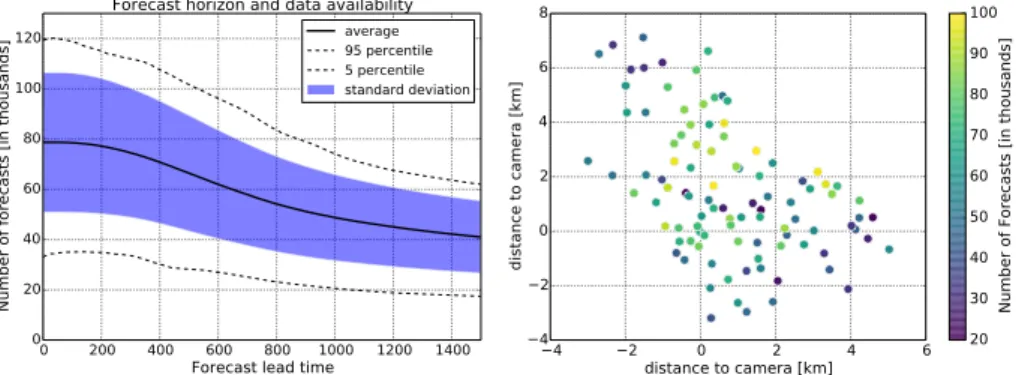
To analyse the performance of our forecasting system, we had to take care about data availability and quality. The total number of processed forecast runs is 138 912, corre-sponding to the number of available images processed for sun elevations greater than 10◦. The number of forecasts used for the evaluation is reduced by non-available
mea-5
surements or forecasts. We decided to use only measurements which were flagged by the data provider as “perfect”. As stations were maintained once a week and quality flags were given for the whole week, data gaps are most of the time covering a whole week (Madhavan et al., 2015). As a consequence, a reduced subset of 50 stations with at least 70 % of the maximal possible number of measurements available was used
10
when comparing performance for different stations (Sect. 4.2). Forecast availability for each location is limited by several factors. The size of the underlying grid, the field of view of the camera (we masked out the area beyond 80◦lens angle of incidence), cur-rent cloud base height, cloud speed and direction and the sun position lead to a varying maximum forecast horizon. Figure 7 illustrates the data availability for the evaluation in
15
dependency on the forecast horizon as well as the spatial distribution for a forecast horizon of 10 min.
3.5.2 Error metrics
For measuring the accuracy and performance of the forecast system we used mean bias error MBE (Eq. 8), root mean square error RMSE (Eq. 9), forecast skill FS (Eq. 10)
20
and Accuracy ACC (Eq. 11) in this analysis.
MBE is the average deviation of the forecast or analysisyfrom the measurementx:
MBE=1n n
X
i=1
(xi−yi), (8)
ACPD
15, 26997–27039, 2015Sky imager based solar irradiance
analysis and forecasts
T. Schmidt et al.
Title Page
Abstract Introduction
Conclusions References
Tables Figures
◭ ◮
◭ ◮
Back Close
Full Screen / Esc
Printer-friendly Version Interactive Discussion
Discussion
P
a
per
|
Discussion
P
a
per
|
Discussion
P
a
per
|
Discussion
P
a
per
|
By definition, RMSE is given by
RMSE= v u u
t1
n
n
X
i=1
(xi−yi)2. (9)
Forecast Skill FS is given by
FS=1−
RMSESkyImager
RMSEPersistence
. (10)
A positive FS means that the sky imager based forecast outperforms persistence
5
(Eq. 7).
Accuracy ACC is used for measuring the ratio of the number of correctly predicted states (sunny and cloudy) by all instances:
ACC= TS+TC
TS+TC+FS+FC, (11)
where TS=True sunny, TC=True cloudy, FS=False sunny and FC=False cloudy. For
10
example, a forecast is true sunny, if measured and predictedk∗are>0.7. A forecast is false sunny, if measuredk∗>0.7 and predictedk∗≤0.7.
These error metrics are calculated for each station and forecast horizon separately.
4 Results and discussion
4.1 Cloud type distribution 15
ACPD
15, 26997–27039, 2015Sky imager based solar irradiance
analysis and forecasts
T. Schmidt et al.
Title Page
Abstract Introduction
Conclusions References
Tables Figures
◭ ◮
◭ ◮
Back Close
Full Screen / Esc
Printer-friendly Version Interactive Discussion
Discussion
P
a
per
|
Discussion
P
a
per
|
Discussion
P
a
per
|
Discussion
P
a
per
|
for a single station which had the highest availability. VariabilityV is defined according to Marquez and Coimbra (2012)
V =
v u u
t1
N
N
X
i=1
(k∗(t
i)−k∗(ti−∆t))2=
v u u
t1
N
N
X
i=1
(∆k∗(t
i))2 (12)
with the number of images in each classN and∆tset to 5 min.
As expected, the convective cloud type classes Cu, Ac/Cc and Sc have the highest
5
variability. Stratocumulus Sc in contrast to Cu and Ac/Cc has a high cloud coverage and therefore causes a lower average clear sky index. St/As cause a low variability close to that of clear sky. The non-intuitive variability for scenes classified as clear sky can be traced back to scenes not fully clear but dominantly clear (not shown here). Cb/Ns and Ci/Cs also cause low variability compared to the first three classes. Cu, Sc, and Ac/Cc
10
occurred in about 37 % of the time, while low variability classes except for clear sky occurred in 53 % of the time, 10 % were clear. No big differences can be seen in the cloud motion statistics for all non-clear situations. An average cloud speed of 10 m s−1 has the effect that a cloud will move across the domain in about 33 min from east to west or from north to south, respectively. This number illustrates one aspect of the limits
15
to the forecast horizon. For further evaluation purposes we group the convective type clouds Cu, Sc, Ac/Cc together to a new category “heterogeneous” clouds, while the cloud types St/As, Ci/Cs and the clear sky situations build the category “homogeneous” clouds, as they cause rather low variability in surface solar irradiance.
4.2 Irradiance analysis accuracy 20
Irradiance analysis is evaluated in dependence on the distance of the stations from the camera and according to the different cloud classes.
The spatial distribution of the mean bias error MBE of the GHI analysis (forecast lead timet=0) is shown in Fig. 8 for Cu and clear sky situations. Here, the MBE is given for each of the stations of the subset introduced in Sect. 3.5.1. The MBE distribution
ACPD
15, 26997–27039, 2015Sky imager based solar irradiance
analysis and forecasts
T. Schmidt et al.
Title Page
Abstract Introduction
Conclusions References
Tables Figures
◭ ◮
◭ ◮
Back Close
Full Screen / Esc
Printer-friendly Version Interactive Discussion
Discussion
P
a
per
|
Discussion
P
a
per
|
Discussion
P
a
per
|
Discussion
P
a
per
|
for Cu shows a negative MBE of about −80 W m−2 for stations close to the camera increasing with distance to positive values around 70 W m−2. A similar overestimation for stations close to the camera can also be found for Ac/Cc, Sc and Ci/Cs (not shown here). This is probably explained by the fact that the correction of RBR (Sect. 3.1.1) is too strong in the circumsolar region (affecting these locations) in the presence of the
5
mentioned clouds. As a result, clouds in the circumsolar region are maybe too often misclassified as clear sky and surface irradiance is overestimated in the area around the camera. This phenomenon is not found for St and Ns/Cb situations dominated by (dark) overcast sky not affected by the correction. Moreover, the clear sky MBE distribution in Fig. 8 shows, that the correction performs in average well in clear sky
10
situations as no significant MBE for stations surrounding the camera is present. An increasing tendency in MBE with distance from the camera is also found for the aforementioned types Ac/Cc, Sc, Ci/Cs, while during clear sky or overcast stratus clouds (only clear sky is shown here) it is not present. A similar tendency is identified for RMSE in Fig. 9 showing the cumulus conditions again. However, even if there is
15
a large (absolute) MBE for stations close to the camera, no enhanced RMSE is present. This makes clear that the main contribution to RMSE is the standard deviation of the analysis error (see Sengupta et al. (2015) for the decomposition of the RMSE) and not the MBE.
Several possible explanations for these results can be identified. First, the
perspec-20
tive error increases with distance from the center of the image. As a result, convective clouds with vertical extent (mostly cumulus), which are interpreted as horizontally flat in our scheme, are projected incorrectly if they are seen from their side near the edge of the field of view. Among other things, this leads to an underestimation of gaps in the cloud layer contributing to a positive MBE and RMSE. Furthermore, uncertainties
25
ACPD
15, 26997–27039, 2015Sky imager based solar irradiance
analysis and forecasts
T. Schmidt et al.
Title Page
Abstract Introduction
Conclusions References
Tables Figures
◭ ◮
◭ ◮
Back Close
Full Screen / Esc
Printer-friendly Version Interactive Discussion
Discussion
P
a
per
|
Discussion
P
a
per
|
Discussion
P
a
per
|
Discussion
P
a
per
|
contributes mainly to RMSE. As the temporal and spatial resolution of 1 Hz and 20 m, respectively, is quite high, double penalties in case of small cumulus or broken cloud layers are likely (Gilleland et al., 2009) and enhance RMSE even more. Furthermore, the pixel resolution is reduced for larger lens incidence angles. This leads to a reduced spatial resolution for locations distant from the camera which affects the accuracy of
5
the camera based irradiance analysis.
Moreover, Fig. 9 shows the RMSE introduced, if a single pyranometer is used repre-sentatively for the whole area. It is assumed that the pyranometer closest to the cam-era is the reference sensor and RMSE of its measurements compared to the remaining pyranometers are calculated. As expected, the error increases very fast with distance
10
as the cross-correlation between the sensor pairs is reduced especially in conditions with high GHI variability. It can be stated that the “break-even” distance where the sky imager based irradiance analysis outperforms a single sensor spatial extrapolation for this highly variable cloud conditions is found at a distance between 1 and 2 km from the camera. For other convective cloud types a distance of 2–3 km for Sc and Ac/Cc and
15
6 km for Ns/Cb is found. In case of St/As and Ci/Cs clouds and in clear sky conditions, the analysis error is always larger due to the high sensor pair correlation in these less variable situations.
4.3 Forecast performance
Figure 10 shows the RMSE of the sky imager forecast and its corresponding
persis-20
tence forecasts in dependency on the forecast horizon for the different cloud conditions. Here, the average RMSE of all evaluated pyranometer stations is shown. As expected, the overall forecast error is higher in situations with more variability in cloud cover and therefore in surface solar irradiance. For cumulus clouds (Cu), the RMSE reaches its maximum of almost 250 W m−2 for a forecast horizon of 10 min, while the error is
al-25
ACPD
15, 26997–27039, 2015Sky imager based solar irradiance
analysis and forecasts
T. Schmidt et al.
Title Page
Abstract Introduction
Conclusions References
Tables Figures
◭ ◮
◭ ◮
Back Close
Full Screen / Esc
Printer-friendly Version Interactive Discussion
Discussion
P
a
per
|
Discussion
P
a
per
|
Discussion
P
a
per
|
Discussion
P
a
per
|
imager forecasts cannot outperform persistence under all cloud conditions. Even if per-sistence error increases fast with time, it stays lower than the corresponding determin-istic forecast error during the whole forecast horizon. For cumulus clouds, a decrease in RMSE after about 10 min is visible even for persistence. The reason could be the varying and limited forecast horizon depending on cloud base height, cloud speed and
5
direction, sun position and the location of each pyranometer itself. The limits of the un-derlying domain is a fixed constraint. A detailed analysis (not shown here) revealed that forecast runs with large forecast horizons have lower RMSE value, probably caused by lower cloud speed causing less GHI variability. This is maximally expressed in the cu-mulus cloud class.
10
From Fig. 10 it can also be seen, that the difference between sky imager forecast RMSE and persistence RMSE is much more pronounced for the stratiform cloud types St/As and Ci/Cs. Figure 11 underlines this result as it shows the forecast skill FS for the categories of “homogeneous” and “heterogeneous” clouds defined in Sect. 4.1. While the sky imager based forecasts are able to outperform persistence under
heteroge-15
neous conditions at least for a few stations after about 10 min, the forecast skill under homogeneous conditions is much worse.
In order to determine the influence of the irradiance retrieval based on the binary cloud/sky decision on the forecast error also binary forecasts with the accuracy metric (Eq. 11) are evaluated. It is expected that the forecast performance is higher, if only the
20
two main states sun and shadow are considered, as GHI forecast errors are introduced into our algorithm during conditions in which the measured GHI distribution deviates strongly from our simplified binary model from Sect. 3.3.
The evaluated accuracy for both sky imager based forecasts and persistence is shown in Fig. 12. Obviously, the accuracy for stratus (St) and
nimbostra-25
indi-ACPD
15, 26997–27039, 2015Sky imager based solar irradiance
analysis and forecasts
T. Schmidt et al.
Title Page
Abstract Introduction
Conclusions References
Tables Figures
◭ ◮
◭ ◮
Back Close
Full Screen / Esc
Printer-friendly Version Interactive Discussion
Discussion
P
a
per
|
Discussion
P
a
per
|
Discussion
P
a
per
|
Discussion
P
a
per
|
cating that misclassifications in cloud detection are preceding the irradiance retrieval. Moreover, from our experience we know that the RBR threshold used for cloud detec-tion is not able to distinguish well between thin cirrus clouds and the blue sky. Stra-tocumulus (Sc) also achieves high accuracy larger than 80 % for the whole horizon. In contrast to RMSE, forecast accuracy can outperform persistence from a forecast lead
5
time of 3–4 min on. This indicates that GHI forecast errors for Sc conditions, which are dominated by high cloud coverage, can be refered to a considerable amount to irradiance retrieval errors. For Cu and Ac/Cc, only low improvements can be stated compared to RMSE for continuous forecast verification. As a consequence, other error sources like spatial mismatch dominate the error in this case. Besides, this result is of
10
interest for applications focusing on binary events which is the case for concentrated solar power (CSP) dealing mainly with variations in direct normal irradiance.
In the former section, we identified a spatial “break-even” distance for GHI analy-sis for different cloud classes. Such a “break-even” point can also be identified for an increased temporal GHI variability. Figure 13 displays the RMSE (based on clear sky
15
indexk∗) of a 10 min forecast in dependence on the prevailing variability (Eq. 12) for 10 mink∗ increments. Here, no distinction in cloud classes is made. RMSE and vari-ability are calculated for short moving time windows of 25 min each. The time step between two time windows is one minute resulting in an overlapping database. The lines in Fig. 13 represent the average values of each bin. With that definition,
persis-20
tence forecast errors fall on the diagonal line of the plot. This analysis summarizes the former investigations of forecast errors under specific cloud conditions. In situations of low GHI variability there is only low forecast skill which is increased with increased GHI variability. As these situations are much less frequent (see dash-dotted line in Fig. 13), this skill is not visible in the average error statistics. Therefore, the strength of
determin-25
loca-ACPD
15, 26997–27039, 2015Sky imager based solar irradiance
analysis and forecasts
T. Schmidt et al.
Title Page
Abstract Introduction
Conclusions References
Tables Figures
◭ ◮
◭ ◮
Back Close
Full Screen / Esc
Printer-friendly Version Interactive Discussion
Discussion
P
a
per
|
Discussion
P
a
per
|
Discussion
P
a
per
|
Discussion
P
a
per
|
tions in the covered area, the results are similar with a slightly different “break-even” value (not shown here).
5 Conclusions
A short-term GHI forecast experiment based on hemispheric images of the visible sky was conducted on a large dataset of spatially distributed pyranometers. A processing
5
chain comprising cloud detection, cloud motion, cloud and shadow mapping and irradi-ance retrieval was proposed and applied to sky images retrieved during April and May 2013. The results show, that the forecast performance and the benefit of sky imager based forecasts vary a lot depending on the given cloud conditions. A cloud classifica-tion scheme was used to determine seven different cloud conditions in order to evaluate
10
the performance in more detail. Even though the overall forecast performance is quite low compared to persistence, one has to point out that the skill increases in heteroge-neous cloud conditions leading to increased variability in surface solar irradiance.
The evaluation of the GHI analysis shows the potential of sky imagers for areal irradiance monitoring. The study shows that the sky imager retrieval for distances
15
of more than 1–2 km from the camera under cumulus cloud conditions outperforms a single pyranometer representing the spatial irradiance distribution. This value is in-creased for stratocumulus and altocumulus/cirrocumulus to 2–3 km and for nimbostra-tus/cumulonimbus to 6 km, respectively. As installing several pyranometers in the field of view of a sky imager is very expensive, a camera based areal irradiance monitoring
20
can be beneficial.
The impact of irradiance retrieval on forecast errors is shown by comparing stan-dard GHI forecast errors to a binary forecast evaluation. This indicates potential for improvements by enhancing the irradiance retrieval. We see also potential to improve the model in the handling of multi-layer clouds (accurate cloud base height and cloud
25
ACPD
15, 26997–27039, 2015Sky imager based solar irradiance
analysis and forecasts
T. Schmidt et al.
Title Page
Abstract Introduction
Conclusions References
Tables Figures
◭ ◮
◭ ◮
Back Close
Full Screen / Esc
Printer-friendly Version Interactive Discussion
Discussion
P
a
per
|
Discussion
P
a
per
|
Discussion
P
a
per
|
Discussion
P
a
per
|
of forecast methods, forecast error will be reduced continously in future. Sky imager based analysis and forecast methods can then contribute to site monitoring and short-term forecasting especially in highly variable cloud conditions.
Acknowledgements. The authors are grateful to the Leibniz Institute for Tropospheric Research
TROPOS (Leipzig, Germany) for providing the datasets of the HD(CP)2pyranometer network, 5
ceilometer and sky imager. Special thanks to Andreas Macke, Madhavan Bomidi and the LACROS team from TROPOS. The authors’ work was funded by the European Commission within the Seventh Framework Programme and the project “Performance Plus” (grant agree-ment no: 308991).
References 10
Bernecker, D., Riess, C., Angelopoulou, E., and Hornegger, J.: Continuous short-term irradiance forecasts using sky images, Sol. Energy, 110, 303–315, doi:10.1016/j.solener.2014.09.005, 2014. 26999
Blanc, P. and Wald, L.: A Library for Computing the Relative Position of the Sun and the Earth, Tech. rep., GMES, Paris, France, 2011. 27002
15
Bouguet, J.-Y.: Pyramidal implementation of the affine lucas kanade feature tracker description of the algorithm, Intel Corporation, 5, 1–10, 2001. 27009
Bourges, B., D.: Yearly variations of the Linke turbidity factor, in: Climatic Data Handbook of Europe, Kluwer Academic Publishing, Dordrecht, 61–64, 1992. 27002
Cazorla, A.: Development of a Sky Imager for Cloud Classification and Aerosol Characteriza-20
tion, PhD thesis, Universidad de Granada, Granada, Spain, 2010. 26999
Cazorla, A., Olmo, F. J., and Alados-Arboledas, L.: Development of a sky imager for cloud cover assessment, J. Opt. Soc. Am. A, 25, 29—39, doi:10.1364/JOSAA.25.000029, 2008. 26999 Chow, C. W., Urquhart, B., Lave, M., Dominguez, A., Kleissl, J., Shields, J., and Washom, B.:
Intra-hour forecasting with a total sky imager at the {UC} San Diego solar energy testbed, 25
Sol. Energy, 85, 2881–2893, doi:10.1016/j.solener.2011.08.025, 2011. 26999, 27003 Chu, Y., Pedro, H. T. C., and Coimbra, C. F. M.: Hybrid intra-hour DNI forecasts with
ACPD
15, 26997–27039, 2015Sky imager based solar irradiance
analysis and forecasts
T. Schmidt et al.
Title Page
Abstract Introduction
Conclusions References
Tables Figures
◭ ◮
◭ ◮
Back Close
Full Screen / Esc
Printer-friendly Version Interactive Discussion
Discussion
P
a
per
|
Discussion
P
a
per
|
Discussion
P
a
per
|
Discussion
P
a
per
|
Chu, Y., Li, M., Pedro, H. T. C., and Coimbra, C. F. M.: Real-time prediction intervals for intra-hour {DNI} forecasts, Renew. Energ., 83, 234–244, doi:10.1016/j.renene.2015.04.022, 2015. 26999
Dumortier, D.: The Satellite Model of Turbidity Variations in Europe, Technical report, École Nationale des Travaux Publics de l’État, 1998. 27002
5
Fontoynont, M., Dumortier, D., Heinnemann, D., Hammer, A., Olseth, J., Skarveit, A., Ine-ichen, P., Reise, C., Page, J., Roche, L., Beyer, H. G. and Wald, L.: Satellight: a WWW server which provides high quality daylight and solar radiation data for Western and Central Europe, in: 9th Conference on Satellite Meteorology and Oceanography, American Meteoro-logical Society Ed., Boston, Massachusetts, USA, 434–437, 25–29 May 1998. 27002 10
Fu, C.-L., and Cheng, H.-Y.: Predicting solar irradiance with all-sky image features via regres-sion, Sol. Energy, 97, 537–550, doi:10.1016/j.solener.2013.09.016, 2013. 26999
Gebejes, A. and Huertas, R.: Texture Characterization based on Grey-Level Co-occurrence Matrix, Proceedings ICTIC (Proceedings in Conference of Informatics and Management Sciences), ISBN: 978-80-554-0648-0, ISSN: 1339-9144, vol. 2,issue 1,pp. 375–378, 2013 15
27007
Ghonima, M. S., Urquhart, B., Chow, C. W., Shields, J. E., Cazorla, A., and Kleissl, J.: A method for cloud detection and opacity classification based on ground based sky imagery, Atmos. Meas. Tech., 5, 2881–2892, doi:10.5194/amt-5-2881-2012, 2012. 27004
Gilleland, E., Ahijevych, D., Brown, B. G., Casati, B., and Ebert, E. E.: Intercom-20
parison of spatial forecast verification methods, Weather Forecast., 24, 1416–1430, doi:10.1175/2009WAF2222269.1, 2009. 27016
Hammer, A., Heinemann, D., Lorenz, E., and Lückehe, B.: Short-term forecasting of solar radia-tion: a statistical approach using satellite data, Sol. Energy, 67, 139–150, doi:10.1016/S0038-092X(00)00038-4, 1999. 26999
25
Haralick, R., Shanmugam, K., and Dinstein, I.: Textural features for image classification, IEEE T. Syst. Man Cyb., SMC-3, 610–621, doi:10.1109/TSMC.1973.4309314, 1973. 27007
Heinle, A., Macke, A., and Srivastav, A.: Automatic cloud classification of whole sky images, Atmos. Meas. Tech., 3, 557–567, doi:10.5194/amt-3-557-2010, 2010. 27007
Inman, R. H., Pedro, H. T. C., and Coimbra, C. F. M.: Solar forecasting methods for renewable 30
ACPD
15, 26997–27039, 2015Sky imager based solar irradiance
analysis and forecasts
T. Schmidt et al.
Title Page
Abstract Introduction
Conclusions References
Tables Figures
◭ ◮
◭ ◮
Back Close
Full Screen / Esc
Printer-friendly Version Interactive Discussion
Discussion
P
a
per
|
Discussion
P
a
per
|
Discussion
P
a
per
|
Discussion
P
a
per
|
Johnson, R., Hering, W., and Shields, J.: Automated Visibility and Cloud Cover Measurements with a Solid State Imaging System, SIO Ref. 89-7, GL- TR-89-0061, NTIS No. ADA216906, final rept. 26 September 1984–25 September 1988, Marine Physical Laboratory, Scripps Institution of Oceanography, University of California, San Diego, 1989. 27003
Johnson, R. W., Koehler, T. L., and Shields, J.: Analysis and Interpretation of Simultaneous 5
Multi-Station Whole Sky Imagery, SIO 91-33, PL- TR-91-2214, NTIS No. ADA253685, final rept. 26 Sep 1984–25 Sep 1988, Marine Physical Laboratory, Scripps Institution of Oceanog-raphy, University of California, San Diego, 1991. 27003
Kalisch, J. and Macke, A.: Estimation of the total cloud cover with high temporal resolution and parametrization of short-term fluctuations of sea surface insolation, Meteorol. Z., 17, 10
603–611, 2008. 27001
Kühnert, J., Lorenz, E., and Heinemann, D.: Satellite-based irradiance and power forecasting for the German energy market, in: Solar Energy Forecasting and Resource Assessment, Elsevier Ltd., , p. 504, 2013. 26999
Long, C. N., Sabburg, J. M., Calbó, J., and Pagès, D.: Retrieving cloud characteristics 15
from ground-based daytime color all-sky images, J. Atmos. Ocean. Tech., 23, 633–652, doi:10.1175/JTECH1875.1, 2006. 26999
Lorenz, E. and Heinemann, D.: Prediction of solar irradiance and photovoltaic power, in: Com-prehensive Renewable Energy, vol. 1, Elsevier Ltd., Oxford, 239–292, 2012. 26999
Lorenz, E., Heinemann, D., and Hammer, A.: Short-term forecasting of solar radiation based on 20
satellite data, in: Proceedings of EuroSun 2004, Freiburg, Germany, 841–848, 20–23 June 2004. 26999
Lucas, B. D. and Kanade, T.: An iterative image registration technique with an application to stereo vision, in: Proceedings of the 7th International Joint Conference on Artificial In-telligence – Volume 2, IJCAI’81, Morgan Kaufmann Publishers Inc., San Francisco, CA, 25
USA, available at: http://dl.acm.org/citation.cfm?id=1623264.1623280 (last access: 1 August 2015), 674–679, San Francisco, CA, USA, 1981. 27009
Madhavan, B. L., Kalisch, J., and Macke, A.: Shortwave surface radiation budget network for observing small-scale cloud inhomogeneity fields, Atmos. Meas. Tech. Discuss., 8, 2555– 2589, doi:10.5194/amtd-8-2555-2015, 2015. 27001, 27012
30
ACPD
15, 26997–27039, 2015Sky imager based solar irradiance
analysis and forecasts
T. Schmidt et al.
Title Page
Abstract Introduction
Conclusions References
Tables Figures
◭ ◮
◭ ◮
Back Close
Full Screen / Esc
Printer-friendly Version Interactive Discussion
Discussion
P
a
per
|
Discussion
P
a
per
|
Discussion
P
a
per
|
Discussion
P
a
per
|
Marquez, R. and Coimbra, C. F. M.: Intra-hour DNI forecasting based on cloud tracking image analysis, Sol. Energy, 91, 327–336, doi:10.1016/j.solener.2012.09.018, 2013. 26999 Olmo, F. J., Cazorla, A., Alados-Arboledas, L., Lopez-Alvarez, M. A., Hernandez-Andres, J.,
and Romero, J.: Retrieval of the optical depth using an all-sky CCD camera, Appl. Optics, 47, 182–189, 2008. 26999
5
Perez, R., Lorenz, E., Pelland, S., Beauharnois, M., Van Knowe, G., Hemler Jr., K., Heinemann, D., Remund, J., Müller, S. C., Traunmüller, W., Steinmauer, G., Pozo, D., Ruiz-Arias, J. A., Lara-Fanego, V., Ramirez-Santigosa, L., Gaston-Romero, M., and Po-mares, L. M.: Comparison of numerical weather prediction solar irradiance forecasts in the US, Canada and Europe, Sol. Energy, 94, 305–326, doi:10.1016/j.solener.2013.05.005, 10
2013. 26999
Pfister, G., McKenzie, R. L., Liley, J. B., Thomas, A., Forgan, B. W., and Long, C. N.: Cloud cov-erage based on all-sky imaging and its impact on surface solar irradiance, J. Appl. Meteorol., 42, 1421–1434, doi:10.1175/1520-0450(2003)042<1421:CCBOAI>2.0.CO;2, 2003. 26999, 27003
15
Quesada-Ruiz, S., Chu, Y., Tovar-Pescador, J., Pedro, H. T. C., and Coimbra, C. F. M.: Cloud-tracking methodology for intra-hour {DNI} forecasting, Sol. Energy, 102, 267–275, doi:10.1016/j.solener.2014.01.030, 2014. 26999
Reikard, G.: Predicting solar radiation at high resolutions: a comparison of time series forecasts, Sol. Energy, 83, 342–349, doi:10.1016/j.solener.2008.08.007, 2009. 26999
20
Sayeef, S., Heslop, S., Cornforth, D., Moore, T., Percy, S., Ward, J., Berry, A., and Rowe, D.: Solar Intermittency: Australia’s Clean Energy Challenge: Characterising the Effect of High Penetration Solar Intermittency on Australian Electricity Networks, CSIRO Sydney, Australia, 2012. 26998
Scaramuzza, D.: OCamCalib: Omnidirectional Camera Calibration Toolbox for Matlab, WWW 25
document, available at: https://sites.google.com/site/scarabotix/ocamcalib-toolbox (last ac-cess: 1 August 2015), Scaramuzza, D., University of Zuerich, Suisse, 2014. 27004
Scaramuzza, D., Martinelli, A., and Siegwart, R.: A toolbox for easy calibrating omnidirectional cameras, in: Proceedings to IEEE International Conference on Intelligent Robots and Sys-tems (IROS 2006), Beijing, China, 2006. 27005
30
ACPD
15, 26997–27039, 2015Sky imager based solar irradiance
analysis and forecasts
T. Schmidt et al.
Title Page
Abstract Introduction
Conclusions References
Tables Figures
◭ ◮
◭ ◮
Back Close
Full Screen / Esc
Printer-friendly Version Interactive Discussion
Discussion
P
a
per
|
Discussion
P
a
per
|
Discussion
P
a
per
|
Discussion
P
a
per
|
TSchmidt_CC.pdf (last access: 1 August 2015), Schmidt, T., Oldenburg, Germany, 2015. 27008
Sengupta, M., Habte, A., Kurtz, S., Dobos, A., Wilbert, S., Lorenz, E., Stoffel, T., Renné, D., Gueymard, C., Myers, D., Wilcox, S., Blanc, P. and Perez, R.: Best Practices Handbook for the Collection and Use of Solar Resource Data for Solar Energy Applications, NREL, Denver, 5
Colorado, 2015. 27015
Shi, J. and Tomasi, C.: Good features to track, in: Proceedings CVPR ’94, 1994 IEEE Computer Society Conference on Computer Vision and Pattern Recognition, 593–600, doi:10.1109/CVPR.1994.323794, 1994. 27009
Shields, J. E., Karr, M. E., Tooman, T. P., Sowle, D. H., and Moore, S. T.: The whole sky imager 10
– a year of progress, In Eighth Atmospheric Radiation Measurement (ARM) Science Team Meeting, Tucson, Arizona, 23–27, 1998. 27003
Shields, J. E., Karr, M. E., Burden, A. R., Johnson, R. W., Mikuls, V. W., Streeter, J. R., and Hodgkiss, W. S.: Research toward Multi-site Characterization of Sky Obscuration by Clouds, Tech. rep., DTIC Document, Scripps Institution of Oceanography, San Diego, California, 15
2009. 27003
Tapakis, R. and Charalambides, A. G.: Equipment and methodologies for cloud detection and classification: a review, Sol. Energy, 95, 392–430, doi:10.1016/j.solener.2012.11.015, 2013. 27007
Urquhart, B., Kurtz, B., Dahlin, E., Ghonima, M., Shields, J. E., and Kleissl, J.: Development of 20
a sky imaging system for short-term solar power forecasting, Atmos. Meas. Tech., 8, 875– 890, doi:10.5194/amt-8-875-2015, 2015. 27003
West, S. R., Rowe, D., Sayeef, S., and Berry, A.: Short-term irradiance fore-casting using skycams: motivation and development, Sol. Energy, 110, 188–207, doi:10.1016/j.solener.2014.08.038, 2014. 26999, 27000, 27003, 27009
25
Wolff, B., Lorenz, E., and Kramer, O.: Statistical learning for short-term photovoltaic power pre-dictions, in: Proceedings of DARE 2013 Workshop on Data Analytics for Renewable Energy Integration, 23–27 September 2013, available at: http://www.ecmlpkdd2013.org/wp-content/ uploads/2013/09/dare2013_paper1_wolff.pdf (last access: 1st August 2015), Praque, Czech Republic, 2013. 26999
30