www.biogeosciences.net/11/2325/2014/ doi:10.5194/bg-11-2325-2014
© Author(s) 2014. CC Attribution 3.0 License.
Biogeosciences
Methane and nitrous oxide fluxes across an elevation gradient in the
tropical Peruvian Andes
Y. A. Teh1,*, T. Diem1, S. Jones2, L. P. Huaraca Quispe3, E. Baggs4, N. Morley4, M. Richards4, P. Smith4, and P. Meir2,5
1Department of Earth and Environmental Sciences, University of St Andrews, Scotland, UK 2School of Geosciences, University of Edinburgh, Scotland, UK
3Universidad Nacional de San Antonio Abad del Cusco, Peru
4Institute of Biological and Environmental Sciences, University of Aberdeen, Scotland, UK 5Research School of Biology, Australian National University, Canberra, Australia
*now at: Institute of Biological and Environmental Sciences, University of Aberdeen, Cruickshank Building, St Machar
Drive, Aberdeen, AB24 3UU, Scotland, UK
Correspondence to:Y. A. Teh ([email protected])
Received: 30 September 2013 – Published in Biogeosciences Discuss.: 5 November 2013 Revised: 17 February 2014 – Accepted: 8 March 2014 – Published: 25 April 2014
Abstract.Remote sensing and inverse modelling studies
in-dicate that the tropics emit more CH4 and N2O than
pre-dicted by bottom-up emissions inventories, suggesting that terrestrial sources are stronger or more numerous than pre-viously thought. Tropical uplands are a potentially large and important source of CH4 and N2O often overlooked
by past empirical and modelling studies. To address this knowledge gap, we investigated spatial, temporal and en-vironmental trends in soil CH4 and N2O fluxes across a
long elevation gradient (600–3700 m a.s.l.) in the Kosñi-pata Valley, in the southern Peruvian Andes, that experi-ences seasonal fluctuations in rainfall. The aim of this work was to produce preliminary estimates of soil CH4and N2O
fluxes from representative habitats within this region, and to identify the proximate controls on soil CH4 and N2O
dynamics. Area-weighted flux calculations indicated that ecosystems across this altitudinal gradient were both at-mospheric sources and sinks of CH4 on an annual basis.
Montane grasslands (3200–3700 m a.s.l.) were strong atmo-spheric sources, emitting 56.94±7.81 kg CH4-C ha−1yr−1.
Upper montane forest (2200–3200 m a.s.l.) and lower mon-tane forest (1200–2200 m a.s.l.) were net atmospheric sinks (−2.99±0.29 and −2.34±0.29 kg CH4-C ha−1yr−1,
re-spectively); while premontane forests (600–1200 m a.s.l.) fluctuated between source or sink depending on the season (wet season: 1.86±1.50 kg CH4-C ha−1yr−1; dry season:
−1.17±0.40 kg CH4-C ha−1yr−1). Analysis of spatial,
tem-poral and environmental trends in soil CH4 flux across the
study site suggest that soil redox was a dominant control on net soil CH4 flux. Soil CH4 emissions were greatest from
habitats, landforms and during times of year when soils were suboxic, and soil CH4 efflux was inversely correlated with
soil O2concentration (Spearman’sρ= −0.45,P <0.0001) and positively correlated with water-filled pore space (Spear-man’sρ=0.63,P <0.0001). Ecosystems across the region were net atmospheric N2O sources. Soil N2O fluxes
de-clined with increasing elevation; area-weighted flux calcu-lations indicated that N2O emissions from premontane
for-est, lower montane forfor-est, upper montane forest and montane grasslands averaged 2.23±1.31, 1.68±0.44, 0.44±0.47 and 0.15±1.10 kg N2O-N ha−1yr−1, respectively. Soil N2O fluxes from premontane and lower montane forests exceeded prior model predictions for the region. Comprehensive in-vestigation of field and laboratory data collected in this study suggest that soil N2O fluxes from this region were
primar-ily driven by denitrification; that nitrate (NO−
3)availability
was the principal constraint on soil N2O fluxes; and that soil
moisture and water-filled porosity played a secondary role in modulating N2O emissions. Any current and future changes
in N management or anthropogenic N deposition may cause shifts in net soil N2O fluxes from these tropical montane
1 Introduction
Recent remote sensing and inverse modelling studies indi-cate that the tropics emit more methane (CH4)and nitrous
oxide (N2O) than estimated from prior bottom-up emissions
inventories, suggesting that tropical sources are stronger or more numerous than previously thought (Frankenberg et al., 2008; Frankenberg et al., 2005; Bergamaschi et al., 2009; Fletcher et al., 2004a, b; Hirsch et al., 2006; Huang et al., 2008; Kort et al., 2011). Recent speculation over discrep-ancies in the global tropical CH4 budget have focussed on
the potential role of seasonally flooded wetlands (Melack et al., 2004; Bergamaschi et al., 2009) or vegetation in account-ing for budgetary gaps; the latter actaccount-ing as abiotic produc-ers (Bergamaschi et al., 2007; Keppler et al., 2006), sites of methanogenic activity (Martinson et al., 2010; Covey et al., 2012) or conduits for atmospheric egress from anoxic soils (Gauci et al., 2010; Terazawa et al., 2007; Pangala et al., 2013). Parallel debates over tropical N2O budgets have
in-voked rising agricultural emissions or atmospheric transport processes as possible causes for discrepancies between top-down and bottom-up budgets (Nevison et al., 2007, 2011; Kort et al., 2011).
One potentially important source of CH4 and N2O
over-looked both by bottom-up inventories and top-down studies are fluxes from tropical upland soils (Spahni et al., 2011), because attention has historically focussed on seasonally in-undated wetlands (e.g.várzeain Brazil) (Fung et al., 1991;
Bergamaschi et al., 2009; Melack et al., 2004; Werner et al., 2007), lowland forests, savannas, or pastures (Hall and Mat-son, 1999; Silver et al., 1999; Teh et al., 2005; Werner et al., 2007; Keller et al., 1986, 1993; Verchot et al., 2000; Keller and Reiners, 1994). However, upland ecosystems account for a substantial fraction of land cover in the tropics; in South America alone, upland ecosystems (>500 m a.s.l.) represent more than 8 % of total continental land cover (Eva et al., 2004), while in mountainous countries, such as Peru or other Andean states, upland ecosystems may account for upwards of 80 % of total land cover (Feeley and Silman, 2010). Mea-surements from tropical uplands in Australia (Breuer et al., 2000), Ecuador (Wolf et al., 2012, 2011), Hawaii (Hall and Matson, 1999; von Fischer and Hedin, 2002, 2007), Puerto Rico (Silver et al., 1999; Teh et al., 2005) and Sulawesi (Veldkamp et al., 2008; Purbopuspito et al., 2006) indicate that CH4and N2O fluxes from these environments are
com-parable or greater than those from tropical lowlands, and may therefore be quantitatively important in regional and global atmospheric budgets, particularly if these ecosystems func-tion as regional “hotspots” of gas producfunc-tion or consump-tion (Teh et al., 2011; Waddington and Roulet, 1996). Soil CH4fluxes in tropical uplands are particularly intriguing
be-cause they show no clear regional patterns or trends. While some ecosystems function as net atmospheric sources, oth-ers operate as net atmospheric sinks (Silver et al., 1999; Teh et al., 2005; Veldkamp et al., 2008; von Fischer and Hedin,
2002; Wolf et al., 2011, 2012). Soil N2O fluxes are more
pre-dictable, but are still poorly constrained (Werner et al., 2007); upland ecosystems, like their lowland counterparts, act as net N2O sources, with emission rates modulated by factors such
as soil moisture, water-filled pore space, soil oxygen content, pH, redox potential, C availability, inorganic N availability (NH+
4, NO −
3), or competition for NO −
3 among different soil
sinks (Hall and Matson, 1999; Silver et al., 1999, 2001; Veld-kamp et al., 2008; Wolf et al., 2011; Firestone and Davidson, 1989).
In the Neotropics, data on upland CH4and N2O fluxes are
particularly scarce, with field observations only from Puerto Rico (Silver et al., 1999; Teh et al., 2005) and Ecuador (Wolf et al., 2011, 2012). Because of the limited spatial cover-age and aseasonality of these two regions, it is difficult to draw wider conclusions about the source or sink strength of Neotropical uplands for CH4and N2O, particularly for
ar-eas that experience marked sar-easonality in rainfall or temper-ature. To address these knowledge gaps, we performed a pre-liminary study of soil CH4 and N2O cycling across a long
elevation gradient (600–3700 m a.s.l.) in the Peruvian Andes that experiences seasonal variations in rainfall, and include a wide range of habitats stretching from premontane forests to wet montane grasslands. Our principal objectives were to:
1. quantify spatial (habitat, landform) and temporal (sea-sonal, month-to-month) trends in soil CH4 and N2O
fluxes;
2. evaluate the role of environmental variables in modu-lating soil CH4and N2O dynamics.
Findings from this research will provide the basis for future, more detailed and integrative studies of soil trace gas dynam-ics in seasonal montane tropical ecosystems; and will also enable us to identify the proximate controls on soil CH4and
N2O fluxes in these diverse environments.
2 Methods and materials
2.1 Study site
Table 1.Site characteristics.
Elevation Areal Coverage Mean Annual Mean Annual Bulk density pH Soil C / N Carbon
Band in the Latitude Longitude Temperature Precipitation A horizon A horizon A horizon Landforms Plots Flux
Kosñipata Valley Chambers
(m a.s.l.) Habitat (km2) Site Name (S) (W) (◦C) (mm) (g cm−3) (%) (mesotopes)
600–1200 Premontane forest 7334 Hacienda 12◦53′43′′ 71◦24′04′′ 23.4 5318 0.30 3.4 15 3 ridge, slope, flat 3 15
Villa Carmen
1200–2200 Lower montane forest 8923 San Pedro 13◦2′56′′ 71◦32′13′′ 18.8 2631 0.31 3.4 15 11 ridge, slope, flat 3 15
2200–3200 Upper montane forest 8066 Wayqecha 13◦11′24′′ 71◦35′13′′ 12.5 1706 0.41 3.9 25 47 slope, flat 3 15
3200–3700 Montane grasslands 5859 Tres Cruces 13◦07′19′′ 71◦36′54′′ 11.8 2200 0.36 4.1 14 10 ridge, slope, flat, basin 4 20
2010b). Thirteen sampling plots (approximately 20×20 m each) were established at four different habitats across a gradient spanning 600–3700 m a.s.l., including premontane forest (600–1200 m a.s.l.; n=3 plots), lower montane for-est (1200–2200 m a.s.l.;n=3 plots), upper montane forest (2200–3200 m a.s.l.; n=3 plots), and montane grasslands (3200–3700 m a.s.l.;n=4 plots; colloquially referred to as “puna”) (Fig. 1). In premontane forest, new sampling plots were established in Hacienda Villa Carmen, a 3065 ha bio-logical reserve operated by the Amazon Conservation As-sociation (ACA), containing a mixture of old-growth forest, secondary forest and agricultural plots. Sampling for soil gas fluxes was concentrated in the old-growth portions of the reserve. For lower montane and upper montane forests, sampling plots were established adjacent to or within exist-ing 1 ha permanent samplexist-ing plots established by ABERG. New sampling plots were also established in montane grass-lands to capture a representative range of environmental con-ditions, microforms (1–5 m scale landforms) and mesotopes (100 m–1 km scale landforms) (Belyea and Baird, 2006), as past ABERG studies of the biogeochemistry of montane grasslands were more limited in both intensity and spatial ex-tent (Gibbon et al., 2010; Zimmermann et al., 2010b). Meso-topic features include ridges, slopes, flats and basins. The latter two landforms include wet, grassy lawns with no dis-cernible grade; and peat-filled depressions found in valley bottoms, respectively. Some (although not all) of these basins abut pool or lake complexes. Because of the logistic chal-lenges of sampling over open water, we did not collect data from the pools or lakes, nor from the shoreline. Summary site descriptions are provided in Table 1 with data on site characteristics collated from prior studies (Feeley and Sil-man, 2010; Girardin et al., 2010; Zimmermann et al., 2009, 2010b).
2.2 Soil–atmosphere exchange
Field sampling was performed over a 13-month period from December 2010 to December 2011 for all habitats except premontane forest. Because of circumstances outside our control, only 6-months of data were collected for premon-tane forest, with sampling commencing in July 2011. Soil– atmosphere fluxes were collected monthly, except where flooding or landslides prevented safe access by fieldworkers to the study sites. Gas exchange rates were determined with five replicate gas flux chambers deployed in each of the 13
m asl
Fig. 1.Map of study sites across the Kosñipata Valley, Manu Na-tional Park, Peru.
plots (n=65 flux observations per month). Sampling was spatially stratified to account for mesotope (100 m–1 km) scale variability in redox and hydrologic conditions (Belyea and Baird, 2006); key environmental factors that often regu-late soil–atmosphere trace gas fluxes (Silver et al., 1999; Teh et al., 2011). All representative landforms were sampled in each habitat, including ridges, slopes, flats and basins (Ta-ble 1). This spatial stratification of sampling was justified by a prior pilot study conducted across the entire ABERG eleva-tion gradient (i.e. 220–3700 m a.s.l.), which found significant within- and among-plot variability in fluxes, suggesting the need for spatially explicit sampling (Saiz and Teh, 2009, un-published data;n=75 static chamber measurements;>10 flux measurements per elevation).
each. Each sampling station was instrumented with a cham-ber base, a soil gas equilibration chamcham-ber buried at a depth of 10 cm (Teh et al., 2005), and a piezometer inserted to bedrock or saprolite depth (≤50 cm). Measurements of air temperature, flux chamber temperature, soil temperature (5 and 10 cm depth), atmospheric pressure, soil moisture (0– 20 cm), soil oxygen (O2)concentration and water table depth
were collected concurrent with flux chamber measurements on a daily basis.
Soil–atmosphere fluxes of CH4, N2O and CO2were
deter-mined using a static flux chamber approach (Teh et al., 2011, Livingston and Hutchinson, 1995), although only CH4 and
N2O fluxes are reported here. Static flux chamber
measure-ments were made by enclosing a 0.03 m2 area with
cylin-drical, opaque (i.e. dark), two-component (i.e. base and lid) vented chambers. Chamber bases were permanently installed to a depth of approximately 5 cm and inserted>1 month prior to the commencement of sampling, in order to mini-mize potential artefacts from root mortality following base emplacement (Varner et al., 2003). Chamber lids were fitted with small computer case fans to promote even mixing in the chamber headspace (Pumpanen et al., 2004). Headspace samples were collected from each flux chamber over a 30 min enclosure period, with samples collected at four discrete in-tervals using a gastight syringe. Gas samples were stored in evacuated Exetainers®(Labco Ltd., Lampeter, UK), shipped
to the UK by courier, and subsequently analysed for CH4,
N2O and CO2concentrations with a Thermo TRACE GC
Ul-tra (Thermo Fisher Scientific Inc., Waltham, Massachusetts, USA) at the University of St Andrews. Chromatographic sep-aration was achieved using a Porapak-Q column, and analyte concentrations quantified using a flame ionization detector (FID) for CH4, electron capture detector (ECD) for N2O, and
methanizer-FID for CO2. Instrumental precision was
deter-mined by repeated analysis of standards and was better than 5 % for all detectors. Fluxes were determined by using the R (R Core Team, 2012) HMR package to plot best-fit lines to the data for headspace concentration against time for individ-ual flux chambers (Pedersen et al., 2010). Gas mixing ratios (ppm) were converted to areal fluxes by using the Ideal Gas Law to solve for the quantity of gas in the headspace (on a mole or mass basis), normalized by the surface area of each static flux chamber (Livingston and Hutchinson, 1995).
2.3 Environmental variables
To investigate the effects of environmental variables on trace gas dynamics, we determined soil moisture, soil oxygen con-tent in the 0–10 cm depth, soil temperature, chamber tem-perature and air temtem-perature at the time of flux sampling. In flooded environments (e.g. basins in montane grasslands), water table depth was also measured using piezometers in-stalled to a depth of≤50 cm in the soil. Soil moisture was de-termined using portable moisture probes (ML2x ThetaProbe, Delta-T Device Ltd., Cambridge, UK) inserted into the
sub-strate immediately adjacent to each flux chamber (<5 cm from each chamber base; depth of 0–10 cm). Soil mois-ture content was measured both as volumetric water content (VWC) and water-filled pore space (WFPS), the latter calcu-lated from VWC and bulk density data (Breuer et al., 2000). For sake of brevity, only WFPS numbers are reported in the body of the text, while both VWC and WFPS data are re-ported in tables. Soil O2 concentration was determined by
analysing soil gas with a portable O2meter (Apogee
Instru-ments Ltd., Logan, Utah, USA), collected from soil gas equi-libration chambers (Teh et al., 2005). Soil gas equiequi-libration chambers were constructed from gas-permeable silicone tub-ing (Clark et al., 2001, Kammann et al., 2001), and perma-nently installed to a depth of 0–10 cm, adjacent to each static flux chamber. Soil O2was measured by withdrawing 40 mL
of soil gas from each soil gas equilibration chamber using a stopcock and gastight syringe. The gas sample was then passed through the flow-through head of the O2 meter into
a second syringe. After the O2measurement was made, the
soil gas was re-injected into the soil gas equilibration cham-ber using the second syringe. Dead volumes were flushed prior to sampling to reduce the likelihood of contamination by atmospheric air or by residual stagnant gas within the sampling system. Soil temperature (0–10 cm depth), cham-ber temperature and air temperature was determined using type K thermocouples (Omega Engineering Ltd., Manch-ester, UK). Data on aboveground litterfall, meteorological variables (i.e. photosynthetically active radiation, air temper-ature, relative humidity, rainfall, wind speed, wind direction), continuous plot-level soil moisture and soil temperature mea-surements (10 cm and 30 cm depths) were also collected, but are not reported in this publication.
Available inorganic N (i.e. ammonium, NH+
4; nitrate,
NO−
3; nitrite, NO−2) concentrations were quantified in all
plots using a resin bag approach (Templer et al., 2005). From August 2011 onwards, ion exchange resin bags (n=15 resin bags per elevation) were deployed at the bottom of the rooting zone (i.e. 0–10 cm depth in premontane for-est, lower montane forest and montane grasslands; 0–15 cm in upper montane forest) (Girardin et al., 2010; Zimmer-mann et al., 2010a), following established protocols (Tem-pler et al., 2005). Samples were collected at monthly in-tervals (where possible) for determination of monthly time-averaged NH+
4, NO −
3 and NO −
2 concentrations. For some
Table 2.Summary of soil sampling scheme for denitrification potential experiment.
Elevation Rooting Soil Sample
Band Zone Depth Depth
(m a.s.l.) Habitat Soil samples Incubations (cm) (cm)
600–1200 Premontane forest 11 19 0–10 5–10
1200–2200 Lower montane forest 2 3 0–25 20–25
2200–3200 Upper montane forest 3 5 0–25 20–25
3200–3700 Montane grasslands 6 10 0–10 5–10
2.4 Denitrification potentials and N2O yields
Potential denitrification rates across the elevation sequence were determined by performing an exploratory15N-labelled
nitrate (15N-NO−
3) laboratory tracer study (Baggs et al.,
2003; Bateman and Baggs, 2005). Details of the soil sam-pling scheme for this experiment are summarized in Table 2. Twenty-two soil samples (125–170 g dry soil per sample) were collected from the same depth as the soil resin bags from sites across the elevation sequence, air-dried and then shipped to the UK by courier. A potential caveat associated with collecting soils from just below the zone of highest root density is that it may lead to underestimates of overall rates of denitrification (due to lower labile C availability) or overesti-mates of N2O production rates (as higher labile C availability
in the zone of greatest root density may promote denitrifica-tion to N2)(Davidson, 1991; Firestone et al., 1980; Weier et al., 1993). However, given evidence for the overarching role of NO−
3 availability in regulating N2O fluxes across this
el-evation gradient (see below), we chose to sample soils from the same depths as our measured indices of NO−
3 (i.e. the
soil resin bags), thus enabling us to better establish possible linkages between NO−
3 availability and microbial
denitrifi-cation potential. Moreover, because the soils were collected on a similar basis, results from the potential denitrification experiment are comparable across study sites, enabling us to probe for relative differences among habitats.
Upon arrival in the UK, 50 g dry soil sub-samples were taken from each soil sample and weighed out into 52 700 mL glass vessels for incubation (n=19 for premontane forest, n=3 for lower montane forest, n=5 for upper montane forest,n=10 for montane grasslands). The uneven sample sizes reflect the fact that this experiment was designed as a preliminary scoping exercise to capture a broad range of environmental conditions, microtopographic and mesotopic features in order to quantify the range of variability in den-itrification rates both within and among habitats. Soil sub-samples were initially re-wetted to 20 % volumetric water content, and allowed to pre-incubate for four days. Soils were further moistened at the start of the experiment to achieve a final WFPS of 80 %. A KNO3 solution containing 0.2 mL
of 0.01 M 40 atom %15N-NO−
3 was then added to the soil,
and the glass incubation vessels sealed to initiate the
exper-iment. Control incubations were conducted with soils from each habitat (n=3 per elevation) to correct for the15N nat-ural abundance signature of endogenous N2O and N2
pro-duction. Gas samples were collected at 0, 6, 12, 24, 33 and 48 hours to quantify N2O,15N-N2O and15N-N2
concentra-tions. Gas concentrations and isotope ratios were determined at the University of Aberdeen, using an Agilent 6890 GC fit-ted with an ECD (Agilent Technologies UK Ltd., Working-ham, UK) and a SerCon 20:20 isotope ratio mass spectrome-ter (IRMS) equipped with an ANCA TGII pre-concentration module (SerCon Ltd., Crewe, UK), respectively. Instrumen-tal precision was determined by repeated analysis of stan-dards and was better than 5 % for both the GC and IRMS. Potential denitrification rates were calculated from the differ-ence in the15N atom % excess values of N
2O and N2relative
to the controls. Fluxes of15N-N2O and15N-N2were
deter-mined using the R (R Core Team; http://www.r-project.org) HMR package (as described above) and normalized for soil dry weight. Total denitrification potential (i.e. sum of15 N-N2O plus 15N-N2 fluxes) and N2O yield (i.e. the ratio of 15N-N
2O :15N-N2O flux+15N-N2flux) were also calculated
(Yang et al., 2011).
2.5 Statistical analyses
Table 3.Abiotic environmental variables for each habitat for the wet and dry season. Upper case letters indicate differences among habitats and lower case letters indicate difference among seasons within habitats (Fisher’s LSD,P <0.05). Values reported here are means and standard errors.
Elevation Band Habitat Volumetric Soil Moisture Water-filled pore space Soil Oxygen Soil Temperature Air Temperature
(m a.s.l.) (%) (%) (%) (◦C) (◦C)
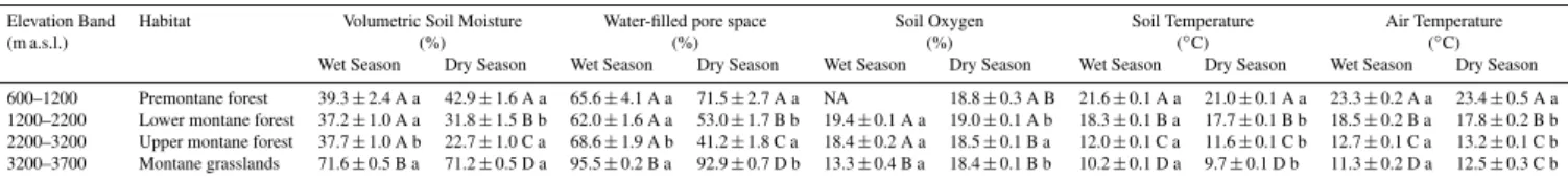
Wet Season Dry Season Wet Season Dry Season Wet Season Dry Season Wet Season Dry Season Wet Season Dry Season 600–1200 Premontane forest 39.3±2.4 A a 42.9±1.6 A a 65.6±4.1 A a 71.5±2.7 A a NA 18.8±0.3 A B 21.6±0.1 A a 21.0±0.1 A a 23.3±0.2 A a 23.4±0.5 A a 1200–2200 Lower montane forest 37.2±1.0 A a 31.8±1.5 B b 62.0±1.6 A a 53.0±1.7 B b 19.4±0.1 A a 19.0±0.1 A b 18.3±0.1 B a 17.7±0.1 B b 18.5±0.2 B a 17.8±0.2 B b 2200–3200 Upper montane forest 37.7±1.0 A b 22.7±1.0 C a 68.6±1.9 A b 41.2±1.8 C a 18.4±0.2 A a 18.5±0.1 B a 12.0±0.1 C a 11.6±0.1 C b 12.7±0.1 C a 13.2±0.1 C b 3200–3700 Montane grasslands 71.6±0.5 B a 71.2±0.5 D a 95.5±0.2 B a 92.9±0.7 D b 13.3±0.4 B a 18.4±0.1 B b 10.2±0.1 D a 9.7±0.1 D b 11.3±0.2 D a 12.5±0.3 C b
Fig. 2. (A)Net CH4and(B)net N2O fluxes by habitat. The short-dash line within each box represents the mean, whereas the solid line represents the median. Boxes enclose the interquartile range, whiskers indicate the 90th and 10th percentiles. The dotted line running across the boxes indicates zero net flux. Kruskal–Wallis ANOVA (P <0.05) was used to test for differences among habi-tats. Lower case letters indicate statistically significant differences among means (Fisher’s LSD on rank transformed data,P <0.05).
used for data that violated assumptions of normality and uni-formity of variances. Relationships among continuous inde-pendent environmental variables and trace gas fluxes were investigated using linear regression for normally distributed data with equal variances, while Poisson regression or Spear-man’s Rank correlation were used to analyse non-normally distributed, heteroscedastic data. Means comparisons were
performed using Fisher’s Least Significant Difference test (Fisher’s LSD). Statistical significance was determined at the P <0.05 level, unless otherwise noted. Values are reported as means and standard errors (±1 SE)
3 Results
3.1 Spatial variation in gas fluxes and environmental
variables
The mean soil CH4 flux for the entire 13-month data
set was 7.79±1.14 mg CH4-C m−2d−1. Soil CH4 fluxes
varied significantly among habitats and over time (GLM, P <0.0001). Multiple comparisons tests indicated that soil CH4 flux from montane grasslands differed significantly
from other habitats (Fisher’s LSD,P <0.05; Fig. 2a). Mon-tane grasslands were net sources of CH4, with a mean flux
of 15.60±2.14 mg CH4-C m−2d−1. In contrast, premon-tane, lower montane and upper montane forests were all net atmospheric sinks, with mean fluxes of −0.16±0.13, −0.64±0.08 and−0.82±0.08 mg CH4-C m−2d−1,
respec-tively (Fig. 2a). Soil CH4fluxes varied significantly among
landforms (Kruskal–Wallis ANOVA, P <0.0001; data not shown). Basin landforms, found only in montane grasslands, emitted significantly more CH4than other landforms (mean
CH4 flux for basin landforms was 63.99±7.80 mg CH4
-C m−2d−1; Fisher’s LSD,P <0.05; data not shown). Other landforms were either weak sources or sinks, but could not be distinguished from each other statistically because of the large variance in fluxes. The mean for pooled soil CH4fluxes from ridge, slope and flat landforms (i.e. the
en-tire data set excluding basin landforms) was 0.47±0.18 mg CH4-C m−2d−1, with a range from−8.71 to 78.5 mg CH4
-C m−2d−1.
The mean soil N2O flux for the entire 13-month
data set was 0.22±0.12 mg N2O-N m−2d−1. N2O fluxes
varied widely among habitats and over time (GLM, P <0.05). Mean N2O fluxes declined progressively with
increasing elevation (Kruskal–Wallis ANOVA, P <0.05), with the highest fluxes observed in premontane forest (0.61±0.36 mg N2O-N m−2d−1), followed by lower
mon-tane forest (0.46±0.12 mg N2O-N m−2d−1), upper
mon-tane forest (0.12±0.13 mg N2O-N m−2d−1)and montane
Fig. 3. (A) Available NH+
4 and (B) available NO−3 fluxes by habitat. The short-dash line within each box represents the mean, whereas the solid line represents the median. Boxes enclose the in-terquartile range, whiskers indicate the 90th and 10th percentiles. Kruskal–Wallis ANOVA (P <0.05) was used to test for differences among habitats. Lower case letters indicate statistically significant differences among means (Fisher’s LSD on rank transformed data,
P <0.05).
Soil N2O fluxes also varied significantly among
land-forms (Kuskal–Wallis ANOVA, P <0.05), with high-est fluxes from flat landforms (0.58±0.23 mg N2 O-N m−2d−1), followed by ridges (0.12±0.25 mg N
2
O-N m−2d−1), slopes (0.06±0.18 mg N
2O-N m−2d−1) and basins (−0.27±0.62 mg N2O-N m−2d−1).
Soil moisture varied significantly among habitats and over time (GLM, P <0.0001). Multiple comparison tests indi-cate that soil moisture varied significantly among habitats (Fisher’s LSD,P <0.05; Table 3). Soil moisture was great-est in montane grasslands (WFPS: 94.7±0.3 %) followed by premontane forest (WFPS: 70.1±2.3 %). Lower mon-tane forest (WFPS: 58.4±1.2 %) and upper montane for-est (WFPS: 58.0±1.6 %) had significantly lower levels of soil moisture than either montane grasslands or premontane forest. Soil moisture varied significantly among landforms
(Kruskal–Wallis ANOVA, P <0.0001). Basins and ridges were significantly wetter than other landforms (WFPS: 97.5±0.2 and 75.1±1.9 %, respectively; Fisher’s LSD, P <0.05; data not shown), while slope and flat landforms showed similar levels of soil moisture (WFPS: 66.8±1.5 and 70.1±1.5 %, respectively).
Soil O2 concentrations in the 0–10 cm soil depth
var-ied significantly among habitats and over time (GLM, P <0.0001). Multiple comparisons tests indicated that soil O2 concentration in montane grasslands was significantly
lower than in other habitats (Fisher’s LSD, P <0.05; Ta-ble 3), with a mean value of 13.8±0.3 %. Mean O2 con-centrations in premontane, lower montane and upper mon-tane forests were 18.7±0.3, 19.2±0.1 and 18.4±0.1 %, respectively. Soil O2 varied significantly among
land-forms (Kruskal–Wallis ANOVA, P <0.0001); basin fea-tures showed significantly lower O2 than other landforms
(5.3±0.9 %; Fisher’s LSD, P <0.05), but other landforms did not differ significantly in O2concentration in the 0–10 cm
soil depth. The pooled mean O2 concentration for ridge,
slope and flat landforms was 17.1±0.2 %, with a range from 0–21 % O2.
Soil and air temperature varied significantly among habi-tats and over time (GLM, P <0.00001 for both soil and air temperature). Multiple comparisons tests indicated that soil and air temperature were significantly different for each habitat (Table 3), with temperatures becoming pro-gressively cooler with increasing elevation (Fisher’s LSD, P <0.05). Temperatures were highest in premontane for-est (soil: 21.2±0.1 C; air: 23.4±0.4 C), followed by lower montane forest (soil: 18.1±0.1 C; air: 18.2±0.1 C), up-per montane forest (soil: 11.8±0.0 C; air: 13.0±0.1 C) and montane grasslands (soil: 10.1±0.1 C; air: 11.8±0.2 C).
Available ammonium (NH+
4) or nitrate (NO −
3)
concen-trations varied significantly among habitats and over time (GLM for NH+
4,P <0.001; GLM for NO −
3,P <0.0001). In
contrast, available NO−
2 concentrations varied widely among
habitats and over time, but with no clear spatial or tempo-ral trends (GLM,P <0.01). For NH+4, multiple comparisons tests indicate that NH+
4concentration was greatest for upper
montane forest, while other habitats did not differ signifi-cantly from each other (Fisher’s LSD, P <0.05; Fig. 3a). NH+
4 concentration for the upper montane forest averaged
17.62±1.33 µg NH+4-N g−1 resin d−1; in contrast, NH+4 concentrations from premontane forest, lower montane forest and montane grasslands averaged 12.28±0.73, 14.82±0.90 and 12.78±0.62 µg NH+
4-N g−1resin d−1, respectively. For
NO−
3, multiple comparisons tests indicate that NO−3
con-centrations decreased significantly with increasing elevation (Fisher’s LSD, P <0.05; Fig. 2b). Mean NO−3 concentra-tions for premontane forest, lower montane forest, upper montane forest and montane grasslands were 17.67±1.70, 12.38±1.87, 4.92±1.57 and 0.17±0.02 µg NO−3-N g−1 resin d−1, respectively. Available NO−
Table 4.Soil methane and nitrous oxide fluxes for each habitat for the wet and dry season. Lower case letters indicate differences among seasons within habitats (Fisher’s LSD,P <0.05). Numbers reported here are means and standard errors.
Methane Flux Nitrous Oxide Flux
Elevation Band (mg CH4-C m−2d−1) (mg N2O-N m−2d−1)
(m a.s.l.) Habitat Wet Season Dry Season Wet Season Dry Season
600–1200 Premontane forest 0.51±0.41 a −0.32±0.11 b −0.15±0.43 a 0.96±0.47 a 1200–2200 Lower montane forest −0.49±0.13 a −0.84±0.07 b 0.16±0.13 a 0.98±0.23 b 2200–3200 Upper montane forest −0.54±0.11 a −1.22±0.04 b 0.02±0.22 a 0.19±0.17 a 3200–3700 Montane grasslands 18.57±2.55 a 0.97±0.47 b −0.61±0.37 a 0.93±0.50 b
not vary significantly among habitats, averaging 0.02±0.00 NO−
2-N g−1resin d−1across the elevation gradient (data not
shown).
3.2 Temporal variability in gas exchange
Soil CH4 efflux increased during the wet season (GLM
P <0.0001; Table 4), although there were no clear direc-tional trends in fluxes within seasons. Furthermore, daily sampling in montane grasslands from 11–22 November 2011 identified no apparent trends in CH4fluxes at this timescale.
Mean soil CH4flux in montane grasslands rose by a factor
of 19 from dry season to wet season, from 0.97±0.47 mg CH4-C m−2d−1in the dry season to 18.57±2.55 mg CH4
-C m−2d−1 (Wilcoxon test,P <0.0001). Likewise net CH4
fluxes became more positive from dry season to wet sea-son for all the other forested habitats (Table 4); the pooled mean for dry season fluxes for the three forest types was −0.86±0.05 mg CH4-C m−2d−1, while the pooled
mean for wet season fluxes was −0.47±0.08 mg CH4 -C m−2d−1 (Wilcoxon test, P <0.0001). This pattern was
most pronounced for premontane forest (Wilcoxon test, P <0.001), where the direction of the soil–atmosphere flux was reversed from a weak atmospheric sink in the dry season (−0.32±0.11 mg CH4-C m−2d−1) to a net atmo-spheric source during the wet season (0.51±0.41 mg CH4
-C m−2d−1).
For the entire data set as a whole, soil N2O fluxes showed
the opposite trend to CH4, with net fluxes declining during
the wet season (Wilcoxon test, P <0.005). However, ac-tual seasonal trends varied among habitats; only fluxes in lower montane forest and montane grasslands changed sig-nificantly between seasons (Wilcoxon tests,P <0.001 and P <0.05, respectively), whereas fluxes in premontane and upper montane forests did not (Table 4).
3.3 Temporal variability in environmental variables
Across the elevation gradient, soil moisture changed signifi-cantly over time, with temporal trends that varied depending on habitat (GLM,P <0.0001). Soil moisture in premontane forest and montane grasslands showed significant month-to-month variability, but did not differ significantly between
seasons (Table 3). In contrast, soil moisture in lower mon-tane and upper monmon-tane forest rose significantly from dry season to wet season, with upper montane forest showing a more pronounced shift in soil water content.
Temporal patterns in soil O2 concentrations varied
depending on habitat. For lower montane forest, soil O2
varied significantly from month-to-month, with small but statistically higher soil O2 observed in the wet season
(19.4±0.1 %) compared to the dry season (19.0±0.1 %) (Wilcoxon test, P <0.001; Table 3). Upper montane forest showed significant month-to-month variability, but no significant differences between seasons (overall mean=18.4±0.1 %). Montane grasslands showed a differ-ent trend from the other habitats, as lower O2concentrations
were observed during the wet season (13.3±0.4 %) com-pared to the dry season (18.4±0.1 %) (Wilcoxon test, P <0.0001; Table 3). Data in the premontane forest site was too sparse to evaluate seasonal patterns in soil O2 content
due to unanticipated delays in the installation of soil gas sampling equipment.
Soil temperature and air temperature varied significantly over time (GLM,P <0.00001 for both soil and air temper-ature). In premontane, lower montane and upper montane forests, the overall trend was towards significantly warmer soil and air temperatures during the wet season (Table 3). Montane grasslands showed a different pattern from the other study sites; no significant seasonal differences in soil temper-ature were observed, while air tempertemper-atures were warmer in the dry season (12.5±0.3◦C) compared to the wet season (11.3±0.2◦C) (Wilcoxon test,P <0.005; Table 3)
There was insufficient data to fully characterize and eval-uate seasonal trends in NH+
4, NO−3 and NO−2 concentrations
as only four months of data were collected over the sampling period. However, significant month-to-month variability was observed in NH+
4, NO−3 and NO−2concentrations.
3.4 Relationships between gas fluxes and environmental
variables
Soil CH4fluxes across the elevation gradient were positively
Fig. 4.Mean plot-level CH4flux against mean plot-level soil O2for the 0–10 cm soil depth. Bars indicate standard errors.
soil CH4flux-soil O2relationship shows clear evidence of a
threshold effect. From 5–21 % soil O2, CH4 efflux is low,
whereas emissions begin to rise steeply below 5 % soil O2
(Fig. 4). When soil CH4fluxes were disaggregated by
habi-tat and season, other relationships emerged, suggesting more habitat-specific controls on soil CH4flux. For example, for
lower montane forest, soil CH4fluxes were negatively
cor-related with soil temperature during the dry season (Spear-man’sρ= −0.64,P <0.01), but not during the wet season.
Only dry season soil N2O fluxes from lower montane
for-est showed any relationship with environmental variables, with N2O fluxes negatively correlated with soil moisture
(Spearman’sρ= −0.41,P <0.1, data not shown). No other trends were found for other habitats or seasons, whether these data were pooled across the entire elevation gradient, or dis-aggregated by habitat and season. There were insufficient data on NH+
4, NO−3 and NO−2 concentrations to statistically
determine if inorganic N fluxes were directly linked to soil N2O emissions.
3.5 Denitrification potentials and N2O yields
Analysis of variance indicated that15N-N
2O,15N-N2and
to-tal denitrification (i.e.15N-N
2O+15N-N2flux) fluxes varied
significantly among habitats (Kruskal–Wallis ANOVA for N2O,P <0.05; Kruskal–Wallis ANOVA for N2,P <0.05;
Kruskal–Wallis ANOVA for total denitrification,P <0.1). The broad overall trend is that upper montane forest showed the lowest fluxes of15N-N2O,15N-N2and total
denitrifica-tion, whereas lower montane forest showed the highest fluxes of 15N-N2O and total denitrification (the latter driven by
the high15N-N
2O component flux). Premontane forest and
montane grasslands showed intermediate fluxes of15N-N 2O, 15N-N
2and total denitrification.
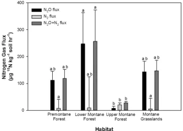
Fig. 5.Potential rates of N2O production, N2production and total (N2O+N2)denitrification from15N-NO−
3 laboratory tracer studies. Kruskal–Wallis ANOVA (P <0.05) was used to test for differences
among habitats. Lower case letters indicate statistically significant differences among means (Fisher’s LSD on rank transformed data,
P <0.05).
For15N-N
2O flux (Fig. 5), premontane forest and
mon-tane grasslands showed comparable fluxes. Lower monmon-tane forest showed the highest flux, while upper montane forest showed the lowest.15N-N
2O flux for lower montane forest
was significantly greater than those for upper montane forest, but within a similar range to premontane forest and montane grasslands (Fisher’s LSD,P <0.05).
For15N-N
2 flux (Fig. 5), premontane forest, lower
for-est and montane grasslands showed comparable fluxes.15
N-N2 flux was significantly greater for upper montane forest
compared to premontane forest or montane grasslands, but within a similar range to lower montane forest (Fisher’s LSD, P <0.05).
Total denitrification flux was highest for lower montane forest, lowest in upper montane forest, and at intermedi-ate levels for premontane forest and montane grasslands. Only lower montane forest and upper montane forest showed significant differences in fluxes (Fisher’s LSD, P <0.05). N2O yields (i.e. ratio of 15N-N2O :15N-N2O flux + 15
N-N2flux) varied significantly among habitats (Kruskal–Wallis
ANOVA, P <0.05; data not shown). Premontane forest, lower montane forest and montane grasslands had statis-tically similar N2O yields (pooled mean of 0.79±0.36), whereas upper montane forest showed the lowest N2O yield
4 Discussion
4.1 Andean ecosystems as both atmospheric sources
and sinks of CH4
Ecosystems across this tropical elevation-gradient functioned as both atmospheric sources and sinks of CH4, further
chal-lenging the long-standing assumption that tropical uplands are only net atmospheric CH4 sinks (Dutaur and Verchot,
2007; Potter et al., 1996; Ridgwell et al., 1999; Teh et al., 2005; von Fischer and Hedin, 2002; Martinson et al., 2010; Covey et al., 2012; Pangala et al., 2013). Soil CH4 fluxes
varied depending on elevation, landform and season. Mon-tane grasslands (3200–3700 m a.s.l.) were net atmospheric sources; upper montane and lower montane forests were net sinks; and premontane forest fluctuated between source or sink depending on the season. From 600–3200 m a.s.l., the sink strength for atmospheric CH4increased with elevation.
This pattern runs counter to observations from elsewhere in Latin America, such as Puerto Rico or Ecuador, where net CH4uptake decreased with increasing elevation (Silver et al.,
1999; Teh et al., 2005; Wolf et al., 2012). The divergence be-tween this study and others is likely due to local and regional differences in precipitation and soil moisture retention. Rain-fall and soil moisture content decreases with rising elevation in this part of the Andes (Girardin et al., 2010), with the no-table exception of montane grasslands, where soil moisture is elevated relative to other habitats across this elevation gradi-ent due to low relief and poor drainage. In contrast, because of regional differences in climate and meteorology, soil mois-ture increases with elevation in Puerto Rico and Ecuador, favouring greater soil anaerobiosis, enhanced methanogene-sis and diminished methanotrophy with rising altitude (Silver et al., 1999; Teh et al., 2005; Wolf et al., 2012).
Soil CH4 fluxes within habitats varied with landforms,
with those in lower topographic positions (e.g. basins) emit-ting more CH4 than those higher up (e.g. ridges). The
de-velopment of more suboxic conditions in lower topographic positions likely drives greater methanogenesis and reduced methanotrophy, a common pattern observed in many other CH4-emitting ecosystems (Teh et al., 2011; von Fischer
et al., 2010; Waddington and Roulet, 1996; Silver et al., 1999). Across the entire altitudinal gradient, basins in mon-tane grasslands emitted more CH4than any other landform,
releasing 233.56±28.47 kg CH4-C ha−1yr−1. Our findings
are in general agreement with studies in Puerto Rico, where higher net soil CH4fluxes were observed from lower
topo-graphic positions (Silver et al., 1999); but differs from re-search in Ecuador, where no significant difference was found in net soil CH4 fluxes among landforms within an
altitudi-nal band (Wolf et al., 2012). The most likely explanation for this divergence between the Peruvian and Puerto Rican tran-sects on one hand, and the Ecuadorian transect on the other, is that the investigators in the latter study sampled only ridge and slope landforms, and did not sample landforms in lower
topographic positions such as flats or basins, presumably be-cause they were less common across this study site (Wolf et al., 2012). In addition, Wolf et al. (2012) did not sample more water-saturated montane grasslands. Landforms in lower to-pographic positions and montane grasslands tend to accumu-late water and contain more reduced soils capable of emitting CH4, unlike more aerobic ridges and slopes that drain more
freely (Teh et al., 2011; von Fischer et al., 2010; Waddington and Roulet, 1996; Silver et al., 1999).
Soil CH4 fluxes varied substantially depending on
sea-son, with an overall shift towards greater CH4 emission
or significant weakening of net soil sinks during the rainy season. These patterns were most pronounced for mon-tane grasslands and premonmon-tane forest; the former showed a nineteen-fold increase in net CH4 efflux from dry
sea-son to wet (0.97±0.47 to 18.57±2.55 mg CH4-C m−2d−1),
while the latter switched from a net atmospheric sink (−0.32±0.11 mg CH4-C m−2d−1) to a net atmospheric
source (0.51±0.41 mg CH4-C m−2d−1). These seasonal
trends differ significantly from Puerto Rico and Ecuador, where soil CH4 fluxes did not vary strongly on an
intra-annual basis, presumably because of weaker rainfall season-ality in these other regions (Silver et al., 1999; Teh et al., 2005; Wolf et al., 2012). However, these data are consistent with findings from other seasonally dry tropical ecosystems, where greater net soil CH4 efflux is associated with wetter
periods of the year, where soil anaerobiosis is more preva-lent (Davidson et al., 2008; Verchot et al., 2000)
Our analysis of spatial, temporal and environmental trends in soil CH4fluxes across the elevation gradient suggest that
soil redox is the principal control on CH4 flux, as is the
case elsewhere in the tropics (Teh et al., 2005; Verchot et al., 2000; von Fischer and Hedin, 2007). Soil CH4emissions
were greatest from habitats and landforms where, or during times of year when, soils were at their most suboxic. This conclusion is further supported by the positive correlation between net soil CH4flux and WFPS, and the negative
corre-lation observed between net soil CH4flux and soil O2(Silver
et al., 1999; Teh et al., 2005).
4.2 Andean ecosystems as atmospheric sources of N2O
Ecosystems across the Kosñipata Valley were net sources of atmospheric N2O. Fluxes progressively declined with
elevation, with lower elevation habitats emitting sub-stantially greater amounts of soil N2O (premontane
for-est: 2.23±1.31 kg N2O-N ha−1yr−1; lower montane
for-est: 1.68±0.44 kg N2O-N ha−1yr−1) than higher
eleva-tion ones (upper montane forest: 0.44±0.47 kg N2
O-N ha−1yr−1; montane grasslands: 0.15±1.10 kg N2
O-N ha−1yr−1). Fluxes from lower elevation habitats ex-ceeded the predictions for bottom-up emissions inven-tories for the region (<0.5–1.0 kg N2O-N ha−1yr−1)
Table 5.Preliminary area-weighted flux estimates for the Kosñipata Valley, Manu National Park, Peru. Surface areas and fractional areas calculated from data published in Feeley and Silman (2010). Fluxes values reported here are means and standard errors.
Unweighted Annual Soil Fluxes Area-weighted Annual Soil Fluxes
Elevation Band Surface Area CH4 N2O CH4 N2O
(m a.s.l.) Habitat (ha) Fractional Area kg CH4-C ha−1yr−1 kg N2O-N ha−1yr−1 kg CH4-C ha−1yr−1 kg N2O-N ha−1yr−1
600–1200 Premontane forest 733 000 0.24 −0.51±0.47 2.23±1.31 −0.14±0.12 0.54±0.32
1200–2200 Lower montane forest 892 000 0.30 −2.34±0.29 1.68±0.44 −0.69±0.09 0.50±0.13
2200–3200 Upper montane forest 807 000 0.27 −2.99±0.29 0.44±0.47 −0.80±0.08 0.12±0.13
3200–3700 Montane grasslands 586 000 0.19 56.94±7.81 0.15±1.10 11.05±1.52 0.03±0.21
TOTALS 3 020 000 1.00 9.42±1.80 1.18±0.79
0.31±0.12 kg N2O-N ha−1yr−1; range of −0.05–1.27 kg
N2O-N ha−1yr−1)(Wolf et al., 2011). Although the cause
for the differences between these observations and prior stud-ies is unclear, it may be linked to the higher N status of lower elevation soils in the Kosñipata Valley, which tend to be more N-rich than soils in Ecuador (Wolf et al., 2011; Fisher et al., 2013; van de Weg et al., 2009).
Analysis of the field and laboratory data suggests that con-trols on soil N2O fluxes in the Kosñipata Valley are complex
and not easily reducible to simple predictive metrics. How-ever, holistic examination of these combined data sets sug-gests that the availability of N, particularly NO−
3, may play
a pivotal role in limiting soil N2O emissions across the
el-evation gradient. The central role of N availability in reg-ulating N2O fluxes is highlighted by the altitudinal trends
in N2O fluxes, available NO−3 concentrations, potential N2O
and N2production, and15N-N2O yields. Even though
poten-tial denitrification rates were roughly similar across the ele-vation gradient (with the exception of upper montane forest), net N2O fluxes and NO−3 availability declined with elevation.
Taken together, these data collectively suggest that altitudi-nal trends in N2O fluxes were due to variations in
denitri-fication, driven by differences in NO−
3 availability. Data on
denitrification potential in upper montane forest further re-inforces this interpretation of the data; upper montane for-est had lower N2O production potential, higher N2
produc-tion potential and lower N2O yields than other sites – all
characteristics reflective of NO−
3-limitation of denitrification
(Blackmer and Bremner, 1978, Weier et al., 1993, Yang et al., 2011). These data are in broad agreement with findings from Ecuador, where N availability was inversely proportional to altitude and was found to be the dominant control on N2O
efflux (Wolf et al., 2011).
Soil WFPS appeared to play a more minor role in modu-lating soil N2O fluxes; a surprising finding given the
promi-nent role played by WFPS in regulating soil N2O fluxes in
other seasonally dry tropical ecosystems (Davidson et al., 2008, Davidson and Verchot, 2000, Davidson et al., 2000, Davidson et al., 1993, Keller and Reiners, 1994). Variations in WFPS only appeared to predict soil N2O fluxes in lower
montane forest during the dry season, and did not predict N2O fluxes in other habitats or during other seasons. This
suggests that WFPS did not limit N2O production during this
13-month period of observation, and that other factors more strongly constrained N2O fluxes in these habitats.
Comprehensive inspection of the environmental data (in-cluding soil moisture, WFPS and available N) suggests that the nature of the constraints on N2O production differ for
each habitat. For premontane forest, lower montane forest and montane grasslands, WFPS fell within a relatively nar-row range, making it potentially difficult to identify the “sig-nal” of WFPS relative to background environmental “noise”, given the complexity of drivers for N2O production
(David-son and Verchot, 2000; Groffman et al., 2009). This signal-to-noise problem is further compounded by the fact that WFPS for these habitats falls within the theoretical range where WFPS no longer limits N2O production from
denitri-fication (i.e. 60–90 %) (Davidson and Verchot, 2000; David-son, 1991). As a consequence, N2O fluxes no longer
in-crease linearly with WFPS, because denitrification rates are near saturation. The high WFPS for these habitats may also explain the seasonal decrease in N2O fluxes from dry to
wet season (Table 4); as these wet soils become increas-ingly waterlogged, denitrification to N2may be increasingly
favoured (Weier et al., 1993). In addition, for montane grass-lands, low NO−
3 availability and high soil C content may
fur-ther promote complete denitrification (Blackmer and Brem-ner, 1978; Davidson, 1991, Weier et al., 1993; Yang et al., 2011; Firestone et al., 1980). In contrast, for upper mon-tane forest, WFPS did in fact vary significantly between sea-sons (Wilcoxon test,P <0.0001; wet season: 68.6±1.9 %; dry season: 41.2±1.8 %). However, N2O flux in this
habi-tat showed no evident response to changes in WFPS, proba-bly because overall denitrification rates were ultimately con-strained by low NO−
3 availability, and high soil C content
drove denitrification to N2(Weier et al., 1993; Firestone et
al., 1980).
4.3 Preliminary area-weighted flux estimates for the
Kosñipata Valley
The high mean annual soil CH4 emission from
mon-tane grasslands (56.94±7.81 kg CH4-C ha−1yr−1)and high
mean annual soil N2O fluxes from premontane and lower
that the Kosñipata Valley is a stronger source for soil CH4
and N2O than previously predicted by bottom-up emissions
inventories for upland tropical ecosystems in the region. To explore this possibility, we performed simple area-weighted flux calculations to estimate the potential contribution of dif-ferent habitats to regional CH4 and N2O exchange. While
we acknowledge that this “back-of-the-envelope” approach is not sufficient to accurately scale up plot-level fluxes to the regional scale, we believe it is still useful as a means of pro-ducing first order approximations of the source or sink po-tential of the region for CH4and N2O.
Using published surface area estimates for different habi-tats for the Kosñipata Valley (Feeley and Silman, 2010), we calculated the areal fractions for each habitat, multiply-ing these values by the mean annual fluxes of soil CH4 or
N2O for our study sites, in order to derive area-weighted
soil flux estimates for each habitat (Table 5). To estimate the regional atmospheric flux of CH4 or N2O (i.e. for the
Kosñipata Valley as a whole), we added together the area-weighted soil fluxes from each habitat (Table 5). This exer-cise produced mean annual flux estimates of 9.42±1.80 kg CH4-C ha−1yr−1and 1.18±0.79 kg N2O-N ha−1yr−1,
re-spectively. This approach may underestimate the true emis-sions potential of these habitats, given that our calculations only accounted for soil-derived fluxes, and did not include estimates of plant-derived fluxes nor emissions from rivers, pools and lakes (Covey et al., 2012; Martinson et al., 2010; Pangala et al., 2013).
The positive sign of the area-weighted soil CH4flux
indi-cates that the region as whole is probably a net atmospheric CH4source, strongly influenced by the contribution of
mon-tane grasslands acting as a regional “hotspot” for CH4. This
speculation is supported by evidence from remote sensing studies showing elevated atmospheric CH4 concentrations
in the tropical Andes, implying the presence of strong re-gional sources, such as waterlogged, suboxic/anoxic mon-tane grasslands (i.e.puna or páramo), unaccounted for by past bottom-up emissions inventories (Wania et al., 2007; Bergamaschi et al., 2007). Likewise the estimated regional soil N2O flux for the Kosñipata Valley exceeds both model
predictions for the region (<0.5–1.0 kg N2O-N ha−1yr−1)
(Werner et al., 2007) and observations from comparable ecosystems in Ecuador (mean annual flux of 0.31±0.12 kg N2O-N ha−1yr−1)(Wolf et al., 2011), probably influenced by the strong emissions from lower elevation habitats, which account for∼54 % of overall land cover.
While these area-weighted flux estimates may only be a first approximation, they are significant because these cal-culations suggest that Andean ecosystems may behave dif-ferently than previously thought, and may be larger emis-sion sources than predicted. These findings also highlight the need for more intensive modelling studies to scale up plot-level measurements to the regional scale in order to more thoroughly evaluate the importance of these ecosystems for regional atmospheric budgets.
5 Conclusions
These data suggest that tropical Andean ecosystems are po-tentially important contributors to regional atmospheric bud-gets of CH4and N2O, and that these ecosystems need to be
considered more fully in future efforts to model and scale up CH4and N2O fluxes from the terrestrial tropics. Ecosystems
across this tropical elevation-gradient were both atmospheric sources and sinks of CH4, challenging long-standing
as-sumptions from the literature that upland tropical ecosystems are only net atmospheric CH4sinks. Simple area-weighted
flux calculations suggest that high soil CH4fluxes from
emis-sions “hotspots” (e.g. montane grasslands) may make the re-gion as a whole a net atmospheric CH4source. This inference
is supported by top-down remote sensing data that indicates the existence of strong local CH4sources in the tropical
An-des, leading to enhanced atmospheric CH4 concentrations.
Soil CH4fluxes were modulated by redox dynamics, with the
largest emissions arising from habitats and landforms where, or during time periods when, soil O2availability was lowest
or soil WFPS was highest. Ecosystems across this altitudi-nal gradient were also net atmospheric sources of N2O, with
the largest soil N2O emissions originating from lower
eleva-tion habitats (premontane forest, lower montane forest). Sim-ple area-weighted flux calculations suggest that this region is likely to be a stronger source of atmospheric N2O than
pre-viously predicted by bottom-up emissions inventories. This is largely due to the fact that lower elevation habitats are rel-atively large emission sources, and account for a substantial fraction of total land area in the region (∼54 %). Proximate controls on soil N2O fluxes were complex and difficult to
elu-cidate from field measurements alone, although comprehen-sive inspection of combined field and laboratory data indicate that NO−
3 availability is the principal constraint on soil N2O
efflux, while soil moisture and water-filled porosity played a secondary role in modulating emissions. Any current and future changes in N management or anthropogenic N depo-sition may cause shifts in net soil N2O fluxes from these
trop-ical montane ecosystems, further enhancing this potentially large emission source.
Supplementary material related to this article is available online at http://www.biogeosciences.net/11/ 2325/2014/bg-11-2325-2014-supplement.zip.
Acknowledgements. The authors would like to acknowledge the
holder and Patrick Meir is supported by an Australian Research Council Fellowship (FT110100457). Javier Eduardo Silva Es-pejo, Walter Huaraca Huasco, Adan Julian Ccahuana and the ABIDA NGO provided critical fieldwork and logistical support. Angus Calder and Vicky Munro provided invaluable laboratory support. Viktoria Oliver provided data on soil characteristics for Hacienda Villa Carmen. Thanks to Adrian Tejedor from the Amazon Conservation Association, who provided assistance with site access and selection at Hacienda Villa Carmen. Thanks are also owed to TCH for providing comments on an earlier draft of this manuscript. This publication is a contribution from the Scottish Alliance for Geoscience, Environment and Society (http://www.sages.ac.uk).
Edited by: P. Stoy
References
Baggs, E. M., Richter, M., Cadisch, G., and Hartwig, U. A.: Denitri-fication in grass swards is increased under elevated atmospheric CO2, Soil. Biol. Biochem., 35, 729–732, 2003.
Bateman, E. J. and Baggs, E. M.: Contributions of nitrification and denitrification to N2O emissions from soils at different water-filled pore space, Biol. Fertil. Soils, 41, 379–388, 2005. Belyea, L. R. and Baird, A. J.: Beyond the limits to peat bog growth:
Cross-scale feedback in peatland development, Ecol. Monogr., 76, 299–322, 2006.
Bergamaschi, P., Frankenberg, C., Meirink, J. F., Krol, M., Den-tener, F., Wagner, T., Platt, U., Kaplan, J. O., Korner, S., Heimann, M., Dlugokencky, E. J., and Goede, A.: Satellite char-tography of atmospheric methane from SCIAMACHY onboard ENVISAT: 2. Evaluation based on inverse model simulations, J. Geophys. Res.-Atmos., 112, 1–26, 2007.
Bergamaschi, P., Frankenberg, C., Meirink, J. F., Krol, M., Villani, M. G., Houweling, S., Dentener, F., Dlugokencky, E. J., Miller, J. B., Gatti, L. V., Engel, A., and Levin, I.: Inverse modeling of global and regional CH4emissions using SCIAMACHY satellite retrievals, J. Geophys. Res.-Atmos., 114, 1–28, 2009.
Blackmer, A. M. and Bremner, J. M.: Inhibitory effect of nitrate on reduction of N2O to N2by soil microorganisms, Soil Biol. Biochem., 10, 187–191, 1978.
Breuer, L., Papen, H., and Butterbach-Bahl, K.: N2O emission from tropical forest soils of Australia, J. Geophys. Res.-Atmos., 105, 26353–26367, 2000.
Clark, M., Jarvis, S., and Maltby, E.: An improved technique for measuring concentration of soil gases at depth in situ, Commun. Soil Sci. Plant Anal., 32, 369–377, 2001.
Covey, K. R., Wood, S. A., Warren, R. J., Lee, X., and Bradford, M. A.: Elevated methane concentrations in trees of an upland forest, Geophys. Res. Lett., 39, L15705, 15701–15706, 2012.
Davidson, E. A.: Fluxes of nitrous oxide and nitric oxide from ter-restrial ecosystems, in: Microbial production and consumption of greenhouse gases: methane, nitrogen oxides, and halomethanes, edited by: Rogers, J. E., and Whitman, W. B., American Society for Microbiology, Washington DC, 219–236, 1991.
Davidson, E. A., Matson, P. A., Vitousek, P. M., Riley, R., Dunkin, K., Garciamendez, G., and Maass, J. M.: Processes regulating soil emissions of NO and N2O in a seasonally dry tropical forest, Ecology, 74, 130–139, 1993.
Davidson, E. A. and Verchot, L. V.: Testing the Hole-in-the-Pipe Model of nitric and nitrous oxide emissions from soils using the TRAGNET Database, Global Biogeochem. Cy., 14, 1035–1043, 2000.
Davidson, E. A., Verchot, L. V., Cattanio, J. H., Ackerman, I. L., and Carvalho, J. E. M.: Effects of soil water content on soil res-piration in forests and cattle pastures of eastern Amazonia, Bio-geochemistry, 48, 53–69, 2000.
Davidson, E. A., Nepstad, D. C., Ishida, F. Y., and Brando, P. M.: Effects of an experimental drought and recovery on soil emis-sions of carbon dioxide, methane, nitrous oxide, and nitric oxide in a moist tropical forest, Glob. Change Biol., 14, 2582–2590, 2008.
Dutaur, L. and Verchot, L. V.: A global inventory of the soil CH4 sink, Global Biogeochem. Cy., 21, 1–9, 2007.
Eva, H. D., Belward, A. S., De Miranda, E. E., Di Bella, C. M., Gond, V., Huber, O., Jones, S., Sgrenzaroli, M., and Fritz, S.: A land cover map of South America, Glob. Change Biol., 10, 731– 744, 2004.
Feeley, K. J. and Silman, M. R.: Land-use and climate change effects on population size and extinction risk of Andean plants, Glob. Change Biol., 16, 3215-3222, 10.1111/j.1365-2486.2010.02197.x, 2010.
Firestone, M. K. and Davidson, E. A.: Microbiological basis of NO and N2O production and consumption in soil, Exchange of Trace Gases between Terrestrial Ecosystems and the Atmo-sphere, edited by: Andreae, M. O. and Schimel, D. S., John Wiley & Sons, New York, 7–21, 1989.
Firestone, M. K., Firestone, R. B., and Tiedge, J. M.: Nitrous oxide from soil denitrification: Factors controlling its biological pro-duction, Science, 208, 749–751, 1980.
Fisher, J. B., Malhi, Y., Torres, I. C., Metcalfe, D. B., van de Weg, M. J., Meir, P., Silva-Espejo, J. E., and Huasco, W. H.: Nutrient limitation in rainforests and cloud forests along a 3000-m eleva-tion gradient in the Peruvian Andes, Oecologia, 172, 889–902, 2013.
Fletcher, S. E. M., Tans, P. P., Bruhwiler, L. M., Miller, J. B., and Heimann, M.: CH4sources estimated from atmospheric observa-tions of CH4and its C-13/C-12 isotopic ratios: 1. Inverse mod-eling of source processes, Global Biogeochem. Cy., 18, 1–17, 2004a.
Fletcher, S. E. M., Tans, P. P., Bruhwiler, L. M., Miller, J. B., and Heimann, M.: CH4sources estimated from atmospheric ob-servations of CH4and its C-13/C-12 isotopic ratios: 2. Inverse modeling of CH4fluxes from geographical regions, Global Bio-geochem. Cy., 18, 1–15, 2004b.
Frankenberg, C., Meirink, J. F., van Weele, M., Platt, U., and Wag-ner, T.: Assessing methane emissions from global space-borne observations, Science, 308, 1010–1014, 2005.
Frankenberg, C., Bergamaschi, P., Butz, A., Houweling, S., Meirink, J. F., Notholt, J., Petersen, A. K., Schrijver, H., Warneke, T., and Aben, I.: Tropical methane emissions: A re-vised view from SCIAMACHY onboard ENVISAT, Geophys. Res. Lett., 35, 1–5, 2008.
Gauci, V., Gowing, D. J. G., Hornibrook, E. R. C., Davis, J. M., and Dise, N. B.: Woody stem methane emission in mature wetland alder trees, Atmos. Environ., 44, 2157–2160, 2010.
Gibbon, A., Silman, M. R., Malhi, Y., Fisher, J. B., Meir, P., Zim-mermann, M., Dargie, G. C., Farfan, W. R., and Garcia, K. C.: Ecosystem Carbon Storage Across the Grassland-Forest Transi-tion in the High Andes of Manu NaTransi-tional Park, Peru, Ecosystems, 13, 1097–1111, 2010.
Girardin, C. A. J., Malhi, Y., AragÃO, L. E. O. C., Mamani, M., Huaraca Huasco, W., Durand, L., Feeley, K. J., Rapp, J., Silva-Espejo, J. E., Silman, M., Salinas, N., and Whittaker, R. J.: Net primary productivity allocation and cycling of carbon along a tropical forest elevational transect in the Peruvian Andes, Glob. Change Biol., 16, 3176–3192, 2010.
Groffman, P. M., Butterbach-Bahl, K., Fulweiler, R. W., Gold, A. J., Morse, J. L., Stander, E. K., Tague, C., Tonitto, C., and Vidon, P.: Challenges to incorporating spatially and temporally explicit phenomena (hotspots and hot moments) in denitrification mod-els, Biogeochemistry, 93, 49–77, 2009.
Hall, S. J. and Matson, P. A.: Nitrogen oxide emissions after nitro-gen additions in tropical forests, Nature, 400, 152–155, 1999. Hirsch, A. I., Michalak, A. M., Bruhwiler, L. M., Peters, W.,
Dlugo-kencky, E. J., and Tans, P. P.: Inverse modeling estimates of the global nitrous oxide surface flux from 1998-2001, Global Bio-geochem. Cy., 20, 1–17, 2006.
Huang, J., Golombek, A., Prinn, R., Weiss, R., Fraser, P., Sim-monds, P., Dlugokencky, E. J., Hall, B., Elkins, J., Steele, P., Lan-genfelds, R., Krummel, P., Dutton, G., and Porter, L.: Estimation of regional emissions of nitrous oxide from 1997 to 2005 using multinetwork measurements, a chemical transport model, and an inverse method, J. Geophys. Res.-Atmos., 113, 1-19, 2008. Kammann, C., Grunhage, L., and Jager, H. J.: A new sampling
tech-nique to monitor concentrations of CH4, N2O and CO2in air at well-defined depths in soils with varied water potential, Euro-pean J. Soil Sci., 52, 297–303, 2001.
Keller, M. and Reiners, W. A.: Soil atmosphere exchange of nitrous oxide, nitric oxide, and methane under secondary succession of pasture to forest in the Atlantic lowlands of Costa Rica, Global Biogeochem. Cy., 8, 399–409, 1994.
Keller, M., Kaplan, W. A., and Wofsy, S. C.: Emissions of N2O, CH4 and CO2 from tropical forest soils, J. Geophys. Res.-Atmos., 91, 1791–1802, 1986.
Keller, M., Veldkamp, E., Weltz, A., and Reiners, W.: Effect of pas-ture age on soil trace-gas emissions from a deforested area of Costa Rica, Nature, 365, 244–246, 1993.
Keppler, F., Hamilton, J. T. G., Brass, M., and Rockmann, T.: Methane emissions from terrestrial plants under aerobic condi-tions, Nature, 439, 187–191, 2006.
Kort, E. A., Patra, P. K., Ishijima, K., Daube, B. C., Jimenez, R., Elkins, J., Hurst, D., Moore, F. L., Sweeney, C., and Wofsy, S. C.: Tropospheric distribution and variability of N2O: Evidence for strong tropical emissions, Geophys. Res. Lett., 38, 1–5, 2011. Livingston, G. and Hutchinson, G.: Chapter 2: Enclosure-based measurement of trace gas exchange: applications and sources of error, in: Biogenic Trace Gases: Measuring Emissions from Soil and Water, edited by: Matson, P., Harriss, RC, Blackwell Science Ltd, Cambridge, MA, USA, 14–51, 1995.
Malhi, Y., Silman, M., Salinas, N., Bush, M., Meir, P., and Saatchi, S.: Introduction: Elevation gradients in the tropics: laboratories
for ecosystem ecology and global change research, Glob. Change Biol., 16, 3171–3175, 2010.
Martinson, G. O., Werner, F. A., Scherber, C., Conrad, R., Corre, M. D., Flessa, H., Wolf, K., Klose, M., Gradstein, S. R., and Veld-kamp, E.: Methane emissions from tank bromeliads in neotropi-cal forests, Nature Geosci., 3, 766–769, 2010.
Melack, J. M., Hess, L. L., Gastil, M., Forsberg, B. R., Hamilton, S. K., Lima, I. B. T., and Novo, E.: Regionalization of methane emissions in the Amazon Basin with microwave remote sensing, Glob. Change Biol., 10, 530–544, 2004.
Nevison, C. D., Mahowald, N. M., Weiss, R. F., and Prinn, R. G.: Interannual and seasonal variability in atmospheric N2O, Global Biogeochem. Cy., 21, 1–13, 2007.
Nevison, C. D., Dlugokencky, E., Dutton, G., Elkins, J. W., Fraser, P., Hall, B., Krummel, P. B., Langenfelds, R. L., O’Doherty, S., Prinn, R. G., Steele, L. P., and Weiss, R. F.: Exploring causes of interannual variability in the seasonal cycles of tro-pospheric nitrous oxide, Atmos. Chem. Phys., 11, 3713–3730, doi:10.5194/acp-11-3713-2011, 2011.
Pangala, S. R., Moore, S., Hornibrook, E. R. C., and Gauci, V.: Trees are major conduits for methane egress from tropical forested wet-lands, New Phytol., 197, 524–531, 2013.
Pedersen, A. R., Petersen, S. O., and Schelde, K.: A comprehensive approach to soil-atmosphere trace-gas flux estimation with static chambers, European J. Soil Sci., 61, 888–902, 2010.
Potter, C. S., Davidson, E. A., and Verchot, L. V.: Estimation of global biogeochemical controls and seasonality in soil methane consumption, Chemosphere, 32, 2219–2246, 1996.
Pumpanen, J., Kolari, P., Ilvesniemi, H., Minkkinen, K., Vesala, T., Niinisto, S., Lohila, A., Larmola, T., Morero, M., Pihlatie, M., Janssens, I., Yuste, J. C., Grunzweig, J. M., Reth, S., Subke, J. A., Savage, K., Kutsch, W., Ostreng, G., Ziegler, W., Anthoni, P., Lindroth, A., and Hari, P.: Comparison of different chamber techniques for measuring soil CO2efflux, Agr. Forest Meteorol., 123, 159–176, 2004.
Purbopuspito, J., Veldkamp, E., Brumme, R., and Murdiyarso, D.: Trace gas fluxes and nitrogen cycling along an elevation se-quence of tropical montane forests in Central Sulawesi, Indone-sia, Global Biogeochem. Cy., 20, 1–11, 2006.
R Core Team: A language and environment for statistical comput-ing, R Foundation for Statistical Computcomput-ing, Vienna, Austria, http://www.R-project.org/, 2012.
Ridgwell, A. J., Marshall, S. J., and Gregson, K.: Consumption of atmospheric methane by soils: A process-based model, Global Biogeochem. Cy., 13, 59–70, 1999.
Silver, W., Lugo, A., and Keller, M.: Soil oxygen availability and biogeochemistry along rainfall and topographic gradients in up-land wet tropical forest soils, Biogeochemistry, 44, 301–328, 1999.
Silver, W. L., Herman, D. J., and Firestone, M. K. S.: Dissimila-tory Nitrate Reduction to Ammonium in Upland Tropical Forest Soils, Ecology, 82, 2410–2416, 2001.