www.biogeosciences.net/11/5245/2014/ doi:10.5194/bg-11-5245-2014
© Author(s) 2014. CC Attribution 3.0 License.
Methane and nitrous oxide sources and emissions in a subtropical
freshwater reservoir, South East Queensland, Australia
K. Sturm1, Z. Yuan1, B. Gibbes2, U. Werner1, and A. Grinham1,2
1Advanced Water Management Centre (AWMC), The University of Queensland, Level 4, Gehrmann Building, Brisbane,
Queensland 4072, Australia
2School of Civil Engineering, The University of Queensland, Level 5, Advanced Engineering Building, Brisbane,
Queensland 4072, Australia
Correspondence to:A. Grinham (a.grinham@uq.edu.au)
Received: 31 October 2013 – Published in Biogeosciences Discuss.: 11 December 2013 Revised: 7 August 2014 – Accepted: 30 August 2014 – Published: 30 September 2014
Abstract. Reservoirs have been identified as an important source of non-carbon dioxide (CO2) greenhouse gases with
wide ranging fluxes for reported methane (CH4); however,
fluxes for nitrous oxide (N2O) are rarely quantified. This
study investigates CH4and N2O sources and emissions in a
subtropical freshwater Gold Creek Reservoir, Australia, us-ing a combination of water–air and sediment–water flux mea-surements and water column and pore water analyses. The reservoir was clearly a source of these gases as surface wa-ters were supersaturated with CH4 and N2O. Atmospheric
CH4 fluxes were dominated by ebullition (60 to 99 %)
rel-ative to diffusive fluxes and ranged from 4.14×10² to 3.06×10⁵µmol CH4m−2day−1 across the sampling sites. Dissolved CH4 concentrations were highest in the anoxic
water column and sediment pore waters (approximately 5 000 000 % supersaturated). CH4 production rates of up to
3616±395 µmol CH4m−2day−1 were found during sedi-ment incubations in anoxic conditions. These findings are in contrast to N2O where no production was detected during
sediment incubations and the highest dissolved N2O
concen-trations were found in the oxic water column which was 110 to 220 % supersaturated with N2O. N2O fluxes to the
atmo-sphere were primarily through the diffusive pathway, mainly driven by diffusive fluxes from the water column and by a minor contribution from sediment diffusion and ebullition. Results suggest that future studies of subtropical reservoirs should monitor CH4fluxes with an appropriate spatial
reso-lution to ensure capture of ebullition zones, whereas assess-ment of N2O fluxes should focus on the diffusive pathway.
1 Introduction
Methane (CH4) and nitrous oxide (N2O) are powerful
green-house gases (GHGs) and are of emerging environmental concern. Their global warming potentials (GWPs) are 25 and 310 times that of carbon dioxide (CO2), respectively,
when calculated on a 100-year time horizon (IPCC, 2007). Man-made reservoirs, which include those for hydropower, agriculture or drinking water purposes, are now considered significant contributors of these GHGs, particularly CH4
(Barros et al., 2011; Bastviken et al., 2011; St. Louis et al., 2000). The recognition of reservoirs as anthropogenic sources of GHGs has thus increased global interest in the measurement, monitoring and modelling of these emissions. The result is a discontinuous database of a large range of pri-marily CH4fluxes, of which studies in potentially important
areas, such as the tropics and subtropics as well as whole con-tinents like Australia, remain scarce (Mendonça et al., 2012; Ortiz-Llorente and Alvarez-Cobelas, 2012; St. Louis et al., 2000). Fewer studies conducted worldwide have analysed the contribution of N2O to GHG emissions from reservoirs
(Guerin et al., 2008; Mengis et al., 1997; Tremblay et al., 2005) despite N2O having a higher GWP than CH4. There
are currently only two studies (Bastien and Demarty, 2013; Grinham et al., 2011) reporting CH4emissions and none for
N2O from reservoirs in Australia – a country with over 2300
reservoirs covering a surface area in excess of 5700 km2at
full supply (Geoscience Australia, 2004).
without continuous release through a dam but may have pe-riodic release for environmental flows and drinking water supplies. These reservoirs enable storage and greater cer-tainty of supply compared to river and groundwater sources in Australia. In reservoirs without continuous water re-lease, the primary CH4emission pathways to the atmosphere
are ebullition from sediments, diffusion over the water–air interface and plant-mediated transport from littoral zones (Bastviken et al., 2004). Ebullition has been shown to be the dominant CH4 emission pathway in many tropical
sys-tems (DelSontro et al., 2011; Devol et al., 1988; Grinham et al., 2011; Joyce and Jewell, 2003; Keller and Stallard, 1994; Soumis et al., 2005). Factors controlling CH4 ebullition in
lake systems are relatively well known (Bastviken et al., 2004; Joyce and Jewell, 2003; Ortiz-Llorente and Alvarez-Cobelas, 2012); however, the dynamics and the spatial dis-tribution of ebullition are not well understood (DelSontro et al., 2011; Ostrovsky et al., 2008; Ramos et al., 2006). CH4is
typically produced by the process of methanogenesis under anoxic conditions (Canfield et al., 2005) as found in the sed-iment and hypolimnetic zones of a reservoir. However, zones within a reservoir may contain large gradients in dissolved oxygen (DO) availability (such as at the metalimnion under stratified conditions or upper layers of shallow sediments) and promote oxidation of dissolved CH4via methanotrophic
bacteria (Guerin and Abril, 2007), which can greatly reduce diffusive emissions from the water surface.
N2O production or consumption is also associated with
these zones where large DO gradients occur. Under oxic con-ditions, as found in the epilimnion or metalimnion, N2O is
primarily produced as a byproduct of nitrification. At oxic– anoxic boundaries, N2O is produced as an intermediate of
denitrification (Mengis et al., 1997; Ward, 1996) or can be reduced to nitrogen gas during denitrification (Lipschultz et al., 1990; Mengis et al., 1997). In stratified reservoirs, the oxic–anoxic boundaries are found in the water column. In well-mixed systems or at shallow sites, DO can reach the sediment surface, and thus N2O can be produced in the
wa-ter column as well as in the upper layers of sediment. The low-latitude reservoirs of Australia provide ideal con-ditions for GHG production, consumption and emissions. The generally higher temperatures experienced in tropical re-gions drive thermal stratification and a rapid deoxygenation of bottom waters (Barros et al., 2011; Tundisi and Tundisi, 2012). Irregular and heavy precipitation events can lead to the input of high organic carbon loads into the water body (Tundisi et al., 1993). The organic carbon loads together with elevated temperatures and deoxygenated bottom wa-ters of these reservoirs will provide conditions that enhance CH4production and emissions (Demarty and Bastien, 2011;
Fearnside, 1995; Galy-Lacaux et al., 1999). The steep oxy-gen gradients and high ammonium turnover found in sub-tropical reservoirs will likely favour N2O production (Guerin
et al., 2008).
There is recent emphasis to further study CH4emissions
from freshwater reservoirs (Barros et al., 2011; Bastviken et al., 2011; Demarty and Bastien, 2011; St. Louis et al., 2000), and this has stimulated an increase of CH4
monitor-ing. However, studies of N2O emissions are lacking (Mengis
et al., 1997; Seitzinger and Kroeze, 1998) despite N2O
be-ing a more potent GHG than CH4. Although GHG studies
from reservoirs have recently increased, they remain lim-ited, particularly in subtropical/tropical regions of the South-ern Hemisphere (Mendonça et al., 2012; Ortiz-Llorente and Alvarez-Cobelas, 2012; St. Louis et al., 2000). Consequently, through this shortfall a large gap in the understanding of global CH4and N2O emissions persists.
In our study we investigated CH4and N2O emissions,
pro-duction and consumption processes in the Gold Creek Reser-voir in South East Queensland, Australia. The study con-sisted of two main parts. First, a detailed field investigation of the CH4and N2O emission rates at two sites (one deep
and one shallow) by measuring total water–air fluxes as well as water column and pore water concentrations. The detailed study also included sediment–water flux incubations of the shallow site which were conducted in the laboratory to gain further insight of the CH4and N2O production or
consump-tion processes. Secondly, a spatial emission field study fo-cused on total flux (ebullitive and diffusive) measurements and estimated diffusive fluxes was performed to assess the CH4and N2O emissions from shallow and deep sites of the
reservoir. This study examined and validated the spatial and temporal representativeness of the CH4 and N2O emission
data from the two sites of the detailed investigation.
2 Materials and methods 2.1 Site description
Gold Creek Reservoir (27◦45′97′′S, 152◦87′86′′E) is located
in subtropical South East Queensland, 14 km west of the city of Brisbane, Australia. Completed in 1885, the reservoir is one of the oldest reservoirs in Australia and was built for the supply of drinking water to Brisbane (although currently not used for this purpose). Gold Creek Reservoir has a sur-face area of 19 ha and is near the median size for Australian reservoirs. The reservoir has a capacity of 820 000 m3 and
maximum water depth of 11.75 m at full supply. Approxi-mately 65 % of the total storage capacity is within the upper 2 m of the reservoir (Supplement Table S1). The reservoir’s pristine catchment area is 10.5 km2and consists of 98 % open
reservoirs where ebullition is frequently observed (Grinham et al., 2011).
In contrast to many temperate systems and reservoirs used for hydropower, Gold Creek Reservoir experiences water level increases mainly by intensive, irregular precipitation events and subsequent inflows especially during the summer months (e.g. 444 mm in 4 days, January 2013; Bureau of Me-teorology, 2013). Water level decreases are caused by water evaporation due to the warm temperatures (annual mean tem-perature 26.4◦C; Bureau of Meteorology, 2013). As Gold
Creek Reservoir has no regular release of water via dam outlets, the turbulent exchange of CH4 and N2O to the
at-mosphere is restricted to when the reservoir’s capacity is exceeded and water is released over a spillway. The reser-voir is steep-sided with limited colonisation of rooted macro-phytes, limiting the importance of plant-mediated emission pathways. This means that the main emission pathways for Gold Creek Reservoir are ebullition from sediments and dif-fusion via the water–air interface.
Located in a subtropical region, Gold Creek Reservoir has relatively high water temperatures compared with many tem-perate systems. Monthly monitoring of water column profiles using a multi-parameter sonde (YSI 6600, YSI Inc., Yellow Springs, OH, USA) showed seasonal ranges of surface wa-ter temperature from 14◦C in winter (June to August) to
30◦C in summer (December to February) and bottom
wa-ter temperatures ranging between 14 to 16◦C in all seasons.
The water column was oxygenated in the upper 2 m during all seasons and stratified for 10 months of the year. Water column profiles of chlorophylla were taken with a
chloro-phyll fluorometer (Seapoint Sensors Inc., Exeter, NH, USA). Sampling and experiments for this study were conducted in March 2012 and February 2014. During these periods, strat-ified conditions predominated, the reservoir was consistently filled to 90–100 % and experienced no overspill.
In the first part of our study, the detailed investigation was conducted at a shallow site (s4) and a deep site (d7) (Fig. 1; Supplement Table S2). CH4and N2O total water–air fluxes
and water column concentrations from both sites were mea-sured as well as pore water concentrations from the shal-low site s4. Additionally, laboratory incubations of sediments from sampling site s4 were conducted to determine CH4and
N2O production as this site was located at the oxycline zone.
The second part of this study investigated the spatial vari-ability of emissions and focused on total flux measurements and diffusive flux estimates at several shallow sites (s1–s4) and deep sites (d5–d8) (Fig. 1; Supplement Table S2). The data obtained in this study were also used to validate the rep-resentativeness of water–air emission estimates from sites s4 and d7 of the detailed study. The average depth of the shal-low sampling sites, located in the reservoir’s sidearms, was 1.7±0.5 m. The deep sampling sites, with an average depth of 7.9±2.7 m, were generally located in the middle of the reservoir body.
Figure 1.The location of the sampling sites at the Gold Creek
Reservoir, South East Queensland, Australia. Sampling sites are numbered from the shallowest to deepest sites. Water depths were for the sites s1: 1.1 m, s2: 1.7 m, s3: 1.9 m, s4: 2.1 m, d5: 4.4 m, d6: 7.5 m, d7: 9.7 m, d8: 10.2 m during the spatial emission study. The detailed study was undertaken at sites s4 and d7.
2.2 Field measurements
2.2.1 Water–air flux measurements
Total CH4and N2O emission fluxes (both ebullitive and
dif-fusive fluxes) at the water–air interface were determined us-ing anchored surface floatus-ing chambers. Gas accumulation of ebullitive and diffusive water–air fluxes in the chambers over time was used for rate calculations. Diffusive water–air fluxes were estimated using the thin boundary layer (TBL) model (Cole et al., 2010). Ebullitive emissions were calcu-lated by the difference between total (floating chamber) and diffusive (TBL model) fluxes.
The surface floating chambers used are described in Grin-ham et al. (2011) and consisted of a floating platform with six small cylindrical PVC chamber units as replicates each with a volume of 0.00048 m3, and surface area of 0.00583 m2. The chambers were stabilised in the water column by anchoring at two points to the reservoir’s floor using an anchor system that was attached to each chamber at two opposite sides. The ropes used for this were connected to a sub-surface floating buoy which was again connected by ropes to an anchor on the reservoir ground. Sampling-induced disturbances to the water column and sampling-induced ebullition from the sed-iments were minimised by a careful approach and by main-taining boat speeds below 2.5 kn.
floating chambers were lifted out of the water and flushed with air. This sampling procedure was repeated 5 times over 5 consecutive days. During the spatial emission study, sur-face floating chambers with three replicate units per chamber were deployed at sites s1–s4 and at sites d5–d8. In this study, the chamber deployment time was 1 h. After taking gas sam-ples from all chamber units, the chambers were also lifted out of the water and flushed with air. This sampling procedure was repeated 3 times at each site. Gas from the chambers was sampled using a 60 mL syringe with a 0.64 mm needle (Livingstone International Pty. Ltd., Rosebery, NSW, Aus-tralia) and transferred into 12 mL pre-evacuated borosilicate vials (Exetainer, Labco Ltd., Lampeter, UK).
Diffusive water–air fluxes were estimated using the equa-tion:
F =k×1C=k×(Cw−Ceq), (1)
whereF is the flux (µmol m−2day−1),kis the gas transfer
coefficient (m day−1) and1C is the difference between the
gas concentration in the surface water (Cw) and the gas
con-centration in the surface water that is in equilibrium with the air (Ceq) (Cole et al., 2010).
The gas transfer coefficient k was estimated using the
model, Eq. (2), developed by Wanninkhof (1992):
k=a×U102 ×(Sc/600)−x, (2)
where a is 0.31 for short-term winds or 0.39 for steady
winds,U10is the frictionless wind speed (m s−1) normalised
at 10 m, Sc is the Schmidt number for CH4 and N2O and x is a constant depending on the wind speed (x=0.66 for
wind speed < 3 m s−1orx=0.5 for wind speed > 3 m s−1).
The Schmidt numberScwas calculated (Wanninkhof, 1992) using Eqs. (3) and (4) for CH4and N2O, respectively:
Sc(CH4)=1897.8−114.28×t+3.2902×t2
−0.039061×t3, (3)
Sc(N2O)=2055.6−137.11×t+4.3173×t2
−0.054350×t3, (4)
wheret is the temperature in Celsius. The frictionless wind
speedU10 was normalised to a height of 10 m according to
Crusius and Wanninkhof (2003):
U10=1.22×U1, (5)
whereU1is the wind speed at 1 m height (m s−1).
Cwwas measured from a water sample (explained in the
next section), whereasCeq was calculated with the
solubil-ity approaches of Yamamoto et al. (1976) for CH4and Weiss
and Price (1980) for N2O and measured atmospheric
con-centrations before starting the chamber deployment times. A weather transmitter (WXT520, Vaisala, Vantaa, Finland) was installed during all sampling times at site d7 and the average
wind speeds were logged every minute (Supplement Figs. S1 and S2a). The wind speeds used for calculations were aver-aged over 24 h for each of the 5 consecutive measurement days for the detailed study and were averaged over the 1 h sampling intervals for the spatial emission study.
2.2.2 Water column sampling
Water column samples were taken at sites s4 and d7 to de-termine the concentrations of CH4, N2O and for the
nutri-ent levels of ammonium (NH+
4), nitrate (NO−3) and nitrite
(NO−
2). Samples were taken from the epilimnion (20 cm
be-low the water surface) and at the metalimnion depth (2 m) with a 4.2 L Niskin water sampler (Wildco, Wildlife Sup-ply Company, Yulee, FL, USA) daily over the 5 consecu-tive days. At site d7, samples were also taken from the hy-polimnion (8 m depth). All water samples were pressure-filtered through 25 mm diameter, 0.22 µm pore-size filters (Merck Millipore, Billerica, MA, USA). Water samples for CH4 and N2O analyses were injected into pre-evacuated
borosilicate vials using a 12 mL syringe with a 0.64 mm nee-dle, then equilibrated in an inflatable glove bag filled with ultra-high purity nitrogen gas (BOC, Brisbane, Australia) to atmospheric pressure and then stored at 4◦C until analysis.
Water samples used for nutrient analyses were stored in ster-ile 10 mL vials (Sarstedt AG & Co., Nümbrecht, Germany) and frozen until analysis was carried out.
2.2.3 Pore water sampling
To investigate sediments as potential sources of CH4 and
N2O, pore waters were extracted from sediment samples and
analysed for CH4 and N2O concentrations at the shallow
site s4. For this, six undisturbed sediment cores were taken with a gravity corer (Envco Environmental Equipment Sup-pliers, Australia), fitted with acrylic liners (69 mm inner di-ameter, 500 mm long) and sealed with PVC caps. The grav-ity corer used had a 2 m pole which limited the collection depth to a shallow site (i.e. site s4). However, Gold Creek Reservoir is generally shallow, with the main storage capac-ity being within the upper 2 m of the storage (Supplement Table S1). Therefore the oxycline of the reservoir is around the 2 m mark (Supplement Fig. S3a) and most sediments of the reservoir are exposed to oxygen. Thus, sediments of the chosen shallow site may be, at least in terms of oxygen ex-posure, representative for most of the reservoir’s sediments.
laboratory, sediments in the test tubes were centrifuged (Ep-pendorf AG, Hamburg, Germany) for 20 min at 1500g,
with-out pressure or temperature changes. The pore water (super-natant) was removed and stored at 4◦C until analysis for
CH4, N2O, NH+4, NO−3 and NO−2. Sample handling as well
as sample equilibration of the gases followed the same proce-dure as described previously for the water column samples.
2.3 Sediment incubation study
Sediment incubations were conducted in the laboratory to de-termine CH4and N2O sediment–water fluxes from the
shal-low site samples (s4). For this, a second set of six undisturbed sediment core replicate samples were collected at site s4 with a gravity corer as described previously. The collected sedi-ments had a height of 9.79±1.12 cm with an overlying wa-ter column of 40.21±1.12 cm. The covered sediment cores were transferred to the laboratory within 4 h, placed into in-cubators and the top PVC caps were removed. The incuba-tors were filled with surface water from the respective site. The water was adjusted to the in situ temperature (24◦C)
us-ing water chillers. The open sediment cores were left to settle overnight while the water column above each sediment core was gently stirred using a magnetic stirring bar suspended in the water column and propelled by additional stirrer bars ro-tating at 18 rpm adjacent to the incubators. Results from in situ deployments of underwater light loggers (Odyssey pho-tosynthetic active radiation recorders, Dataflow Systems Pty. Ltd., Christchurch, New Zealand) indicated strong light at-tenuation at the reservoir, with the photic zone being less than 1 to 0.5 m (Supplement Fig. S4). Consequently, for these sediment studies the incubators were covered with aluminum foil on the sides and light-blocking cloth at the top to mimic the reservoir’s sediment conditions below the photic zone.
The sediment core liners were capped 15 h after sampling using plexiglas lids with O-rings taking care to exclude air bubbles. The lids contained three ports for sampling, refilling and for a dissolved oxygen probe (tip sealed against sampling port). One-way valves were attached to the tubing (Mas-terflex Tygon, John Morris Scientific Pty. Ltd., Chatswood, NSW, Australia) of the sampling and refilling ports, and a rubber stopper was used for the oxygen probe port if not used. Sampling and refilling with site water were carried out with 20 mL syringes. Dissolved oxygen and temperature of the water column above the sediment cores were moni-tored using an optical DO probe (PreSens, Precision Sensing GmbH, Regensburg, Germany) before the core liners were capped and every 24 h subsequently until the experiment fin-ished. Cores were regularly inspected for signs of ebullition (bubble formation under the cap) throughout the incubation times. Samples from the overlying water of the sediment cores were taken for analysis of CH4, N2O and the nutrients
NH+
4, NO−3 and NO−2 before the cores were capped and after
72, 120 and 288 h incubation. Daily fluxes were determined for CH4, NH+4, NO−3 and NO−2 over 288 h and for DO over
48 h. These were calculated from the rates of change in con-centration and by taking the core volume and sediment sur-face area into account. CH4, N2O and nutrient sample
han-dling as well as sample equilibration of the gases followed the same procedure as described previously for the water col-umn samples.
2.4 Analyses
Both gaseous and liquid samples were analysed for CH4and
N2O concentrations using an Agilent GC7890A gas
chro-matograph (Agilent Technologies, Santa Clara, CA, USA). A flame ionisation detector and a micro-electron capture de-tector were used for the analysis of CH4and N2O,
respec-tively. The gas chromatograph was calibrated using stan-dards with a range of 1.8 to 82 000 ppm for CH4 and 0.5
to 50.53 ppm for N2O which were prepared from certified
gas standards (BOC gases, Brisbane, Australia). A Lachat QuickChem 8000 Flow Injection Analyzer (Lachat Instru-ment, Milwaukee, WI, USA) was used for the analysis of NH+
4, NO−3 and NO−2 concentrations.
Statistical analyses were performed with the program Sta-tistica version 12 (StatSoft Inc., Tulsa, OK, USA), using one-way analysis of variances (ANOVAs). In order to eval-uate differences amongst sampling sites, one-way ANOVAs were performed with sampling sites s4 or d7, sampling days 1–5 or the sampling depths (epilimnion, metalimnion, hy-polimnion, pore water) as the categorical predictor and CH4,
N2O or nutrients (NH+4, NO−3, NO−2) as the continuous
vari-ables. Data were log transformed where necessary to ensure normality of distribution and homogeneity of variance (Lev-ene’s test) (Zar, 1984). Post hoc tests were performed using Fisher’s LSD (least significant difference) test (Zar, 1984). The non-parametric Kruskal–Wallis (KW) test was used for data which failed to satisfy the assumptions of normality and homogeneity of data after being transformed.
3 Results
3.1 Water–air fluxes
Sites s4 (shallow) and d7 (deep) of the detailed study showed significantly different (KW-H1,60=41.2, P <0.001) CH4
emission rates, with the highest rates found at the shallow site s4 (Fig. 2a and c; Table 1). However, there was no signifi-cant difference (P >0.05) found in N2O emissions between
the two sites (Fig. 2b and d; Table 1). Total CH4and N2O
fluxes across the 5 consecutive monitoring days were not sig-nificantly different (P >0.05) at both sampling sites s4 and
d7, apart from N2O fluxes at site s4 between day 4 and day 5
(KW-H9,60=47.8,P <0.01). Results of the detailed study (Fig. 2) showed that diffusive fluxes account for 12 to 40 % of the total CH4fluxes at site d7 and less than 3 % at site s4.
Figure 2.Total and diffusive methane and nitrous oxide fluxes at the shallow sampling site s4(a, b)and the deep sampling site d7(c, d)
determined over 5 consecutive days. Total fluxes were determined from measurements using the anchored surface floating chambers, and diffusive fluxes were determined using the thin boundary layer model. Fluxes are given as averages±SE,n=6.
Table 1. Total water–air methane and nitrous oxide fluxes at the
shallow site s4 and the deep site d7 of the detailed study. Fluxes are given as the average determined over the 5 consecutive days±SE, n=30.
Site Total CH4fluxes Total N2O fluxes (µmol CH4m−2day−1) (µmol N2O m−2day−1)
s4 10 423±1249 2.89±0.17
d7 1210±223 2.01±0.03
N2O fluxes for both sites. Otherwise, the estimated fluxes
exceed the measured fluxes by up to 80 % (Fig. 2b and d; discussed in Sect. 4.1).
The spatial emission study confirmed that the Gold Creek Reservoir is a source of both CH4and N2O (Fig. 3; Table 2).
However, the results show that CH4fluxes varied much more
widely (6300 to 258 535 µmol CH4m−2day−1) than N2O
fluxes (0.73 to 1.40 µmol N2O m−2day−1). No significant
trend was observed for flux differences between shallow and deep sites for either investigated gas, except that CH4
emis-sions at the shallow site s1 exceeded the emisemis-sions of all other sites by 1–2 orders of magnitude. CH4emissions at site
s1 were significantly different (KW-H7,72=41.0,P <0.05) from all other sampling sites, while significant difference was
Table 2.Total water–air methane and nitrous oxide fluxes at
sam-pling sites s1–s4 and d5–d8 of the spatial emission study. Rates are averaged over three surface floating chamber deployments. Sam-pling sites are numbered from shallowest to deepest site. Fluxes are given as an average±SE,n=9.
Site Total CH4fluxes Total N2O fluxes (µmol CH4m−2day−1) (µmol N2O m−2day−1)
s1 258 535±37 087 0.73±0.06
s2 21 381±6695 1.24±0.08
s3 20 452±4164 1.40±0.06
s4 6726±2686 1.20±0.15
d5 28 597±5411 1.10±0.10
d6 30 274±13 023 0.87±0.05
d7 6300±932 1.17±0.08
d8 15 952±1896 1.22±0.08
not detected between emissions from the other sites s2–s4 and d5–d8 (P >0.05). The highest CH4emissions from the
deeper sites were detected at sites d5 and d6, which are both located in the north-western arm of the reservoir close to the shallow site s1. In contrast to this, no clear spatial pat-tern between sites was observed for N2O fluxes. Similarly,
N2O fluxes measured amongst four sites, two shallow and
Figure 3.Total and diffusive methane(a)and nitrous oxide(b)fluxes at sampling sites s1–s4 and d5–d8. Total fluxes were determined
using the anchored surface floating chambers, and diffusive fluxes were determined using the thin boundary layer model. Rates per site were averaged over three surface floating chamber deployments. Sampling sites are numbered from shallowest to deepest. Fluxes are given as average±SE,n=9.
different (P >0.05). However, N2O fluxes from sampling
site d6 were different than all other sites (KW-H7,72=31.2, P <0.01) apart from s1 and d5 (P >0.05). Interestingly,
the lowest N2O fluxes were measured at the shallow site s1.
Comparing total fluxes with diffusive fluxes from all sam-pling sites showed that in the spatial emission study, diffusive fluxes accounted for 1 to 6 % of the total CH4fluxes (Fig. 3a).
Diffusive fluxes explain, in five out of the eight sites, 82 to 100 % of total N2O fluxes; although, at one site, d6, the
dif-fusive flux exceeded (by up to 25 %) the measured total flux (Fig. 3b; discussed in Sect. 4.1).
Wind speed during the spatial emission study (Supplement Fig. S2a) conducted at sites s1–s4 and d5–d8 increased from the first (1.8±0.8 m s−1) to the second (2.8±1.4 m s−1) chamber deployment as well as from the second to the third (4.0±1.2 m s−1) chamber deployment (deployment interval for each floating chamber was 1 h). Averaged chamber N2O
fluxes increased at all sites with increasing wind speed; how-ever, the increase was not significant (P >0.05)
(Supple-ment Fig. S2b). In contrast to this, averaged CH4fluxes at all
sites did not increase with the increasing wind speed (Sup-plement Fig. S2c). Total chamber fluxes of each chamber de-ployment and per sampling site showed low variability for N2O and high variability for CH4.
Averaged total chamber CH4fluxes were not significantly
different (P >0.05) between the two conducted studies
(de-tailed study from March 2012 and spatial emission study from February 2014) for the shallow site s4. However, at the deep site d7, total CH4 fluxes differed significantly
be-tween the two studies (KW-H1,39=18.2,P <0.001). The
total N2O fluxes at both sites, site s4 and site d7, differed
sig-nificantly between the two studies (KW-H1,39=19.1,P <
0.001 andF1,37=124.6,P <0.001, respectively).
3.2 Water column parameters
Water column CH4, N2O and nutrient concentrations at both
sites s4 (Fig. 4a and b; Table 3) and d7 (Fig. 4c and d; Ta-ble 3) showed no significant difference (P >0.05) amongst
the 5 consecutive experiment days and thus were pooled. The reservoir was characterised by a clear stratification with re-spect to oxygen (Supplement Fig. S3a). Epilimnetic layers were fully oxic, while metalimnetic layers were suboxic and the hypolimnetic layer at the deep site d7 was anoxic.
The epilimnion at both sites s4 and d7 was supersatu-rated with CH4and N2O. CH4metalimnion concentrations at
site s4 were 1 order of magnitude higher than the epilimnion concentrations. At site d7, hypolimnion CH4concentrations
were approximately 24 000 000 % supersaturated and 2–3 or-ders of magnitude higher than the meta- and epilimnion con-centrations, respectively. N2O concentrations were
compa-rable for both sites s4 and d7 in the epilimnion and metal-imnion. However, N2O concentrations at site d7 were highest
in the epilimnion, not in the hypolimnion. The epilimnetic and metalimnetic CH4 and N2O concentrations at site s4
were comparable to the measured concentrations at site d7. NH+
4 concentrations at site s4 were not significantly
dif-ferent (P >0.05) in epilimnion and metalimnion. NO−2 and
NO−
3 concentrations at site s4 showed slight increases
be-tween epilimnion and metalimnion. NH+
4 concentrations at
site d7 were similar in the epilimnion and metalimnion but 2 orders of magnitude higher in the hypolimnion. NO−
2 and
NO−
3 concentrations at site d7 were not significantly
differ-ent (P >0.05) within each of the three investigated water
column layers. All analysed NH+
4, NO−2 and NO−3
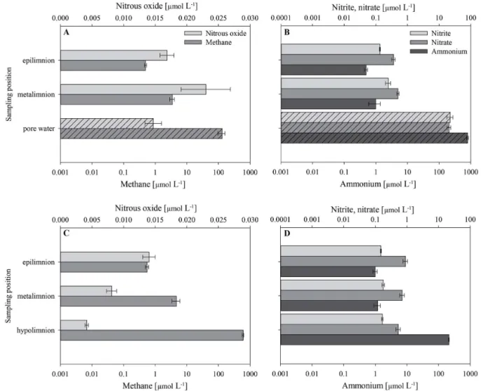
Figure 4.Levels of methane, nitrous oxide and nutrients determined at the shallow sampling site s4(a, b)and at the deep sampling site d7 (c, d). Results are shown for the epilimnion, metalimnion and for pore water (bars with hatch pattern) at the shallow site s4 and for
the epilimnion, metalimnion and hypolimnion at the deep site d7. Methane and nutrient concentrations are plotted on a log scale. Values represent averages±SE with the number of replicates beingn=12 for water column methane and nitrous oxide,n=15 for nutrient water
column samples,n=4 for pore water methane and nitrous oxide andn=8 for pore water nutrients.
3.3 Pore water parameters
The dissolved CH4 pore water concentrations at site s4
(Fig. 4a; Table 3) were 2 orders of magnitude higher than the concentrations measured in the epilimnion as well as in the metalimnion. The pore waters were approximately 5 000 000 % supersaturated with CH4(pore waters were
col-lected from the upper sediment layers and the saturation per-cent was calculated as done for the water samples). N2O
pore water concentrations at site s4 were comparable to mea-sured concentrations in both investigated water column lay-ers (epilimnion and metalimnion). NH+
4 pore water
concen-trations at site s4 (Fig. 4b; Table 3) were 3 orders of mag-nitude higher than in the epilimnion and metalimnion. Sim-ilarly, the pore water NO−
2 and NO−3 concentrations were 2
orders of magnitude higher than in the water column.
3.4 Sediment–water fluxes
CH4 was consistently produced during the incubations of
the site s4 sediments (Fig. 5a, Table 4). N2O concentrations
indicated consumption had occurred; however, these levels were low and near the theoretical detection limit from 72 h onwards (Fig. 5a). Dissolved oxygen was rapidly removed (Table 4) from overlying waters and was not detected after 48 h (Fig. 5a). NH+
4 concentrations increased significantly
(F3,8=6.1, P <0.01) between the start and end (288 h)
of the incubation study. NO−
2 concentrations were seen to
have increased over time following the same pattern as NH+ 4,
while the NO−
Table 3.Measured methane, nitrous oxide and nutrient concentrations of the detailed study at the shallow site s4 in the epilimnion, metal-imnion and pore water and at the deep site d7 in the epilmetal-imnion, metalmetal-imnion and hypolmetal-imnion. Values represent the average±SE:n=12
for water column methane and nitrous oxide;n=15 for water column nutrients;n=4 for pore water methane and nitrous oxide andn=8
for pore water nutrients.
Site Measured Epilimnion Metalimnion Pore water parameter concentration concentration concentration s4 CH
4 0.50±0.04 µmol CH4L
−1 3.47±0.60 129±32
21 986±2660 % saturation µmol CH4L−1 µmol CH4L−1
N2O 0.017±0.001 µmol N2O L−1 0.023±0.004 0.015±0.001 168±12 % saturation µmol N2O L−1 µmol N2O L−1
NH+
4 0.49
±0.06 0.99±0.40 798±51
µmol NH+
4-N L−1 µmol NH+4-N L−1 µmol NH+4-N L−1
NO− 2
0.13±0.00 0.25±0.04 23±5
µmol NO−
2-N L−1 µmol NO−2-N L−1 µmol NO−2-N L−1
NO− 3
0.36±0.05 0.50±0.04 21±3
µmol NO−
3-N L−1 µmol NO−3-N L−1 µmol NO−3-N L−1
Site Measured Epilimnion Metalimnion Hypolimnion parameter concentration concentration concentration d7 CH
4 0.55±0.07 µmol CH4L
−1 4.69±1.29 600±28
19 722±1465 % saturation µmol CH4L−1 µmol CH4L−1
N2O 0.014±0.001 µmol N2O L−1 0.008±0.001 0.004±0.000 206±14 % saturation µmol N2O L−1 µmol N2O L−1
NH+
4 0.99
±0.15 1.18±0.27 212±6
µmol NH+
4-N L−1 µmol NH+4-N L−1 µmol NH+4-N L−1
NO− 2
0.15±0.01 0.18±0.02 0.17±0.01
µmol NO−
2-N L−1 µmol NO−2-N L−1 µmol NO−2-N L−1
NO− 3
0.90±0.15 0.71±0.12 0.53±0.08
µmol NO−
3-N L−1 µmol NO−3-N L−1 µmol NO−3-N L−1
Table 4.Production and consumption rates of methane, nitrous
ox-ide and nutrients during the sediment incubation study. Positive val-ues indicate production and negative valval-ues indicate consumption. Rates are given as an average±SE,n=3.
Measured Production/ parameter consumption rates
CH4 3616±395 µmol CH4m−2day−1
DO −38 220 µmol O2m−2day−1
NH+
4 3874±1129 µmol NH+4-N m−2day−1
NO−
2 17±10 µmol NO−2-N m−2day−1
NO−
3 −8±5 µmol NO−3-N m−2day−1 CH4, NH+4, NO−2, NO−3 production/consumption rates were determined between hour 0 and 288 of the incubation experiment. The DO rate was determined between hour 0 and 48 of the incubation experiment.
4 Discussion
4.1 Surface gas emissions and the dominance of CH4ebullition
The water–air flux measurements of the detailed study as well as the spatial emission study showed that the Gold Creek Reservoir was a source of CH4and N2O. Overall CH4
emis-sions emitted from the water surface were at least 1–2 (de-tailed study) or 2–4 (spatial emission study) orders of mag-nitude higher relative to N2O in terms of CO2 equivalents,
despite N2O being a more powerful GHG than CH4.
The spatial emission study showed high variability of to-tal CH4fluxes across and within (amongst chamber
deploy-ments) all sampling sites and low variability of total N2O
Figure 5. Sediment incubations of the shallow site s4: dissolved
oxygen, methane, nitrous oxide(a)and nutrient production or
con-sumption(b). Values represent averages±SE,n=3.
been observed in other tropical reservoir studies (Bastviken et al., 2010; DelSontro et al., 2011; Grinham et al., 2011).
A comparison of the measured fluxes determined at the floating chambers and the estimated fluxes determined using the TBL model clearly showed that at all the sites the CH4
fluxes were mainly driven by ebullition and the N2O fluxes
were mainly driven by diffusion. Our findings confirm those of previous studies, where ebullition has been shown to pro-duce the largest CH4emissions compared to the pathways of
diffusion and plant-mediated transport. This is especially the case under the conditions of shallow and warm water sys-tems where high CH4 production rates occur (DelSontro et
al., 2011; Devol et al., 1988; Grinham et al., 2011; Joyce and Jewell, 2003; Keller and Stallard, 1994). Gold Creek Reservoir meets those conditions as it is a shallow system (maximum depth of 11.75 m) experiencing warm tempera-tures (Supplement Fig. S3b) throughout the year. Diffusion is the dominant pathway for N2O emissions at Gold Creek
Reservoir and this has been found in other tropical reservoirs (Guerin et al., 2008).
Estimated N2O fluxes in some cases exceeded the fluxes
measured by the floating chambers. It is likely this anomaly results from inherent errors in both these methods. The esti-mates were based on one exemplary model for the gas trans-fer coefficient, k (Wanninkhof, 1992). However, there are
various models described that give over- or underestimations of measured fluxes and wide discrepancies in their results (Musenze et al., 2014; Ortiz-Llorente and Alvarez-Cobelas, 2012). In addition, modelled fluxes can be influenced by a number of factors that include rainfall on the water surface
(Guerin et al., 2007; Ho et al., 1997); spatial variations of wind speed (Matthews et al., 2003); heating and cooling of the water surface (Polsenaere et al., 2013; Rudorff et al., 2011); surrounding vegetation; and wind fetch (Cole et al., 2010). Emission rates in this study were modelled with av-eraged wind speeds forkover the deployment time of 24 h
periods (detailed study) and for 1 h periods (spatial emis-sion study). Diurnal changes in wind speed occurred with higher wind speeds during daylight which was when the spa-tial study was conducted. Therefore, the deployment periods do not provide the same study conditions and could introduce an error; consequently, comparisons of daily rates between the two studies should be treated with caution.
4.2 Factors controlling CH4ebullition
Both studies (detailed and spatial emission) showed that ebullition from anoxic sediments was the main contributor to the total CH4emissions in this subtropical reservoir. The
detailed study showed that ebullitive CH4fluxes were higher
at site s4 than at site d7. The spatial emission study revealed that ebullitive CH4fluxes at site s1 were significantly higher
than at all deep sites. These results confirm findings from Bastviken et al. (2004) showing that CH4fluxes by
ebulli-tion are depth-dependent and higher at water depths of 4 m or less. Ebullition, and ultimately CH4emission, can be
en-hanced when the hydrostatic pressure is reduced which could be a result of current-induced bottom shear stress or the lowering of storage water levels (Joyce and Jewell, 2003; Ostrovsky et al., 2008). The already quite low hydrostatic pressure in the Gold Creek Reservoir (i.e. < 2 atmospheres) favours active ebullition there. The CH4in the gas bubbles
can escape oxidation during the transport through the water column as CH4 moves faster through the water column by
ebullition than by diffusion (Joyce and Jewell, 2003). Inter-estingly, however, significantly higher ebullition rates were not found at the other shallow sites (s2–s4) as compared to the deeper sites. Highest CH4water–air fluxes of the spatial
emission study were generally found at the shallow site s1 and the deep sites d5 and d6, located in the north-western arm of the reservoir. These three sites (s1, d5 and d6) are located where the main water inflow to the reservoir would occur, and these likely receive high amounts of organic matter com-pared to the other sites. Hence, higher CH4production
result-ing in higher fluxes would occur at these sites. This would also explain why CH4 fluxes at the shallow sites s2–s4 did
not support other findings of depth-dependent fluxes as they likely receive less organic matter than received in the north-western sidearm of the reservoir. The chlorophylla profile
surrounding catchment as the highest CH4 flux rates were
found adjacent to major inflows where there was intense for-est litter deposition. This phenomenon has been observed in other storages within the region (Grinham et al., 2011) and highlights the importance of identifying ebullition hot spots to improve total emission estimates.
The CH4fluxes from Gold Creek Reservoir compare well
with other reservoirs (Table 5) in the South East Queensland region (e.g. Little Nerang Dam (Grinham et al., 2011) and Baroon Pocket Dam (Grinham et al., 2012)) and even ex-ceeded the rates of younger reservoirs (e.g. Lake Wivenhoe and Baroon Pocket Dam; Grinham et al., 2012). The age of a reservoir is described as one of the parameters affecting GHG fluxes as it is often described that fluxes tend to decline with the reservoir age (Abril et al., 2005; Galy-Lacaux et al., 1999). Barros et al. (2011) used published data from different hydroelectric reservoirs to show that the relationship between CH4flux and reservoir age is negatively correlated. However,
CH4fluxes from reservoirs measured in South East
Queens-land (Table 5) significantly exceeded the fluxes analysed by Barros et al. (2011), and the older reservoirs in the region showed higher CH4emissions rates than the younger
reser-voirs. This may be explained by intensive, irregular precipi-tation events that occur in the region, and these would period-ically flush high amounts of organic matter into the system. It is likely that these bursts of high organic loadings would allow the ebullitive pathways for CH4 emissions to persist
and maintain high fluxes over time.
4.3 Sources of CH4production
Generally, the highest CH4concentrations in the Gold Creek
Reservoir were found in the hypolimnion and sediments, in-dicating the sediments as a main source of CH4. The
hy-polimnetic CH4concentrations were comparable to
concen-trations found in other stratified, tropical reservoirs (Abril et al., 2005; Galy-Lacaux et al., 1999; Guerin and Abril, 2007). Epilimnetic CH4concentrations were 3 orders of magnitude
lower than concentrations in the hypolimnion, indicating that a substantial portion of the CH4was oxidised by CH4
-oxidising bacteria before reaching the surface waters and the atmosphere, as has been suggested to occur in other tropical reservoirs (Guerin and Abril, 2007; Lima, 2005). These epil-imnion concentrations were comparable (Guerin and Abril, 2007) or significantly lower (up to 3 orders of magnitude) than concentrations found in other stratified, tropical reser-voirs (Abril et al., 2005). Despite lower CH4concentrations
in the epilimnion, the reservoir was still supersaturated with CH4and a source to the atmosphere.
The laboratory incubations showed that the sediments of Gold Creek Reservoir were a consistent source of CH4 as
the CH4concentration steadily increased throughout the
in-cubation period. This supports the findings of the field study where CH4sediment pore water concentrations were greatly
elevated relative to the surface water concentrations. The
Table 5. The range of methane fluxes across selected reservoirs (covering shallow and deep sites) in South East Queensland.
Reservoir Commission CH4flux ranges year (µmol CH4m−2day−1)
Baroon Pocket Dam 1988 505–251 750 (Grinham et al., 2012)
Lake Wivenhoe 1984 95–78 500
(Grinham et al., 2012)
Little Nerang Dam 1962 4230–1 403 250 (Grinham et al., 2011)
Gold Creek Reservoir 1885 414–306 302 (this study)
high methanogenesis rates in the sediments are thus likely driving a significant portion of the water–air CH4 fluxes
measured in this study. Past studies have demonstrated that sediments are a significant CH4source (Barros et al., 2011;
Canfield et al., 2005). A recent study on a similar reservoir system clearly demonstrated the dominance of methanogenic archaea in the upper 15 cm of the sediment zone (Green et al., 2012). Given the high rates of organic matter loading in these systems, CH4production will be an important pathway
for organic matter degradation in the sediments. The highly supersaturated concentrations of the pore waters of this relatively shallow reservoir means that any small changes in hydrostatic pressure, e.g. via bottom shear, would likely increase the ebullition rates (Joyce and Jewell, 2003). In comparison of the CH4sediment–water fluxes with the CH4
water–air fluxes from the shallow site s4, it was evident that the sediment efflux (3616±395 µmol CH4m−2day−1) explained 67 % of the diffusive CH4 emissions
(5400±1250 µmol CH4m−2day−1) and 35 % of the total CH4 emissions (10 423±1249 µmol CH4m−2day−1). This strongly indicates that the fluxes assessed during the sediment incubations in this study were underestimated. The most influential factor for this underestimation is likely the height of the incubated sediment core. With a height of only about 10 cm, the CH4production from deeper (also anoxic)
sediment layers was not considered.
4.4 Sources of N2O production or consumption
The sediment incubation study clearly showed that the anoxic sediments were the source of NH+
4 for the N2O
pro-duction (Fig. 5b). However, N2O production through
ei-ther the nitrification or denitrification pathway ultimately re-quires DO. Dissolved oxygen is introduced into the upper water layer through wind re-aeration or by photosynthetic production. The production of N2O, therefore, suffers from
twin limitations; below the oxycline DO is limiting, whereas above the oxycline, NH+
4 is limiting. This confines N2O
the degree of supersaturation and, therefore, the likelihood of bubble production. The net result was that N2O emissions
from the water surface predominately occurred through the diffusive pathway.
Our measurements showed that the surface waters were supersaturated with N2O so the system was acting as a N2O
source to the atmosphere. The elevated N2O concentrations
in the oxic zones (epilimnion and metalimnion) relative to the anoxic zones indicate that nitrification was the predom-inant production pathway. N2O consumption occurs in the
anoxic hypolimnion and sediments possibly via denitrifica-tion as found previously (Guerin et al., 2008; Mengis et al., 1997). The presence of NO−
3 within the anoxic zones further
supports the likelihood of denitrification.
4.5 Implications
Intensive field and laboratory studies in Gold Creek Reser-voir were undertaken to improve the understanding of pro-duction/consumption and emission rates of the non-CO2
GHGs, CH4 and N2O. Our results clearly demonstrate that
the Gold Creek Reservoir is a source of CH4 and N2O
to the atmosphere although CH4 is clearly the dominant
gas even when expressed as CO2 equivalents. N2O flux
rates were in fact much lower than those reported in other reservoirs with similar climates (N2O fluxes from six
reser-voirs of three countries (Brazil, Panama, French Guiana) ranged between 3–157 µmol N2O m−2day−1(Guerin et al.,
2008); in comparison, the fluxes in this study range be-tween 0.73–2.89 µmol N2O m−2day−1). Gold Creek
Reser-voir CH4fluxes, on the other hand (53 t CH4yr−1; range
be-tween 7–290 t CH4yr−1), were dominated by ebullitive
emis-sions and were within the range reported for other tropi-cal systems (St. Louis et al., 2000). The exception was the flux measured at the shallowest site (s1) which greatly ex-ceeded even the higher-end range from the young (filled in 1994) Petit Saut Dam in French Guiana (Galy-Lacaux et al., 1997; St. Louis et al., 2000). Barros et al. (2011) de-termined that the relationship between CH4 flux and
lati-tude is significantly negatively correlated. CH4fluxes from
Gold Creek Reservoir (spatial emission study range be-tween 6300–258 535 µmol CH4m−2day−1), situated at the
latitude of 27◦45′97′′S, significantly exceeded the fluxes
pre-sented in that study, which were given to be in general less than 4167 µmol CH4m−2day−1. The catchment of the Gold
Creek Reservoir consists of 98 % forest and experiences warm temperatures as well as intense precipitation events that potentially flush high amounts of organic matter into the reservoir throughout the year. These characteristics are in contrast to temperate systems and likely accelerate the CH4production in subtropical systems like the Gold Creek
Reservoir. The high rates of CH4flux that we measured
fur-ther highlight the importance of studies that focus on sub-tropical systems. Additionally, studies from sub-tropical fresh-water systems are also important as these experience higher
water temperatures than subtropical systems and are thus ex-pected to exhibit even higher surface CH4 fluxes (Barros et
al., 2011). There is a lack of study of Australia’s reservoirs in both the tropical and subtropical climate zones, and their contribution as significant CH4 emitters is not recognised.
Future emission studies of these systems would add to the limited knowledge of this region, which is important for in-clusion in global GHG estimates.
The spatial variability results of our study further empha-sise the importance of including a reasonable spatial reso-lution when monitoring GHG emissions from water bodies, particularly when measuring CH4. In addition, monitoring
efforts should include measuring CH4ebullition as it is the
most dominant pathway in these systems. For N2O, however,
assessing only diffusive fluxes is likely sufficient. Our results also suggest that reservoir age is potentially not an important parameter affecting CH4 fluxes in systems similar to Gold
Creek Reservoir. Ultimately, the results presented here are likely to be globally relevant as an increasing number of large reservoirs are being constructed to meet growing water de-mand, particularly in tropical and subtropical zones, but also because subtropical systems can provide insight into the pos-sible impacts that a warming climate will have on temperate reservoirs.
The Supplement related to this article is available online at doi:10.5194/bg-11-5245-2014-supplement.
Acknowledgements. The authors gratefully acknowledge the support and collaboration of Michele Burford at Griffith University. The advice and assistance provided by the RS&T team, Andrew Watkinson and Duncan Middleton of Seqwater are also gratefully acknowledged. We would like to thank Tonya DelSontro for the very helpful guidance provided during the manuscript reviewing process. We thank the three anonymous reviewers whose sugges-tions have greatly improved this manuscript. We also would like to thank Philip Bond for a thorough review of the manuscript. This project was financially supported by the Australian Research Council (ARC) project LP100100325.
Edited by: T. DelSontro
References
Abril, G., Guerin, F., Richard, S., Delmas, R., Galy-Lacaux, C., Gosse, P., Tremblay, A., Varfalvy, L., Dos Santos, M. A., and Matvienko, B.: Carbon dioxide and methane emissions and the carbon budget of a 10-year old tropical reservoir (Petit Saut, French Guiana), Global Biogeochem. Cy., 19, GB4007, doi:10.1029/2005gb002457, 2005.
Bastien, J. and Demarty, M.: Spatio-temporal variation of gross CO2and CH4diffusive emissions from Australian reservoirs and natural aquatic ecosystems, and estimation of net reservoir emis-sions, Lakes & Reservoirs Research and Management, 18, 115– 127, doi:10.1111/lre.12028, 2013.
Bastviken, D., Cole, J., Pace, M., and Tranvik, L.: Methane emis-sions from lakes: Dependence of lake characteristics, two re-gional assessments, and a global estimate, Global Biogeochem. Cy., 18, GB4009, doi:10.1029/2004gb002238, 2004.
Bastviken, D., Santoro, A. L., Marotta, H., Pinho, L. Q., Calheiros, D. F., Crill, P., and Enrich-Prast, A.: Methane emissions from Pantanal, South America, during the low water season: Toward more comprehensive sampling, Environ. Sci. Technol., 44, 5450– 5455, doi:10.1021/es1005048, 2010.
Bastviken, D., Tranvik, L. J., Downing, J. A., Crill, P. M., and Enrich-Prast, A.: Freshwater methane emissions offset the continental carbon sink, Science, 331, 6013, doi:10.1126/science.1196808, 2011.
Canfield, D. E., Erik, K., and Bo, T.: The Methane Cycle, in: Ad-vances in Marine Biology, edited by: Donald, E., Canfield, E. K., and Bo, T., Academic Press, 383–418, 2005.
Climate Data Online, Bureau of Meteorology, Copyright Common-wealth of Australia, available at: www.bom.gov.au, last access: 6 October, 2013.
Cole, J. J., Bade, D. L., Bastviken, D., Pace, M. L., and Van de Bogert, M.: Multiple approaches to estimating air-water gas ex-change in small lakes, Limnol. Oceanogr.-Methods, 8, 285–293, doi:10.4319/lom.2010.8.285, 2010.
Crusius, J. and Wanninkhof, R.: Gas transfer velocities measured at low wind speed over a lake, Limnol. Oceanogr., 48, 1010–1017, 2003.
DelSontro, T., Kunz, M. J., Kempter, T., Wuest, A., Wehrli, B., and Senn, D. B.: Spatial heterogeneity of methane ebullition in a large tropical reservoir, Environ. Sci. Technol., 45, 9866–9873, doi:10.1021/es2005545, 2011.
Demarty, M. and Bastien, J.: GHG emissions from hydroelectric reservoirs in tropical and equatorial regions: Review of 20 years of CH4emission measurements, Energ. Policy, 39, 4197–4206, doi:10.1016/j.enpol.2011.04.033, 2011.
Devol, A. H., Richey, J. E., Clark, W. A., King, S. L., and Mar-tinelli, L. A.: Methane emissions to the troposphere from the Amazon Floodplain, J. Geophys. Res.-Atmos., 93, 1583–1592, doi:10.1029/JD093iD02p01583, 1988.
Fearnside, P. M.: Hydroelectric dams in the Brazilian Amazon as sources of greenhouse gases, Environ. Conserv., 22, 7–19, 1995. Galy-Lacaux, C., Delmas, R., Jambert, C., Dumestre, J.-F., Labroue, L., Richard, S., and Gosse, P.: Gaseous emissions and oxygen consumption in hydroelectric dams: A case study in French Guyana, Global Biogeochemical Cy., 11, 471–483, doi:10.1029/97gb01625, 1997.
Galy-Lacaux, C., Delmas, R., Kouadio, G., Richard, S., and Gosse, P.: Long-term greenhouse gas emissions from hydroelectric reservoirs in tropical forest regions, Global Biogeochem. Cy., 13, 503–517, doi:10.1029/1998gb900015, 1999.
Geoscience Australia: Dams and water storages 1990, available at: www.ga.gov.au, 2004.
Green, T. J., Barnes, A. C., Bartkow, M., Gale, D., and Grinham, A.: Sediment bacteria and archaea community analysis and nutrient
fluxes in a sub-tropical polymictic reservoir, Aquat. Microbial Ecol., 65, 287–302, 2012.
Grinham, A., Dunbabin, M., Gale, D., and Udy, J.: Quantifi-cation of ebullitive and diffusive methane release to atmo-sphere from a water storage, Atmos. Environ., 45, 7166–7173, doi:10.1016/j.atmosenv.2011.09.011, 2011.
Grinham, A., Gibbes, B., Cutts, N., Kvennefors, C., Jinks, D., and Dunbabin, M.: Quantifying natural GHG sources and sinks: Lake Wivenhoe and Baroon Pocket Dam, Seqwater internal report, The University of Queensland, 2012.
Guerin, F. and Abril, G.: Significance of pelagic aerobic methane oxidation in the methane and carbon budget of a tropical reservoir, J. Geophys. Res.-Biogeo., 112, G03006, doi:10.1029/2006jg000393, 2007.
Guerin, F., Abril, G., Serca, D., Delon, C., Richard, S., Delmas, R., Tremblay, A., and Varfalvy, L.: Gas transfer velocities of CO2 and CH4in a tropical reservoir and its river downstream, J. Mar.
Syst., 66, 161–172, doi:10.1016/j.jmarsys.2006.03.019, 2007. Guerin, F., Abril, G., Tremblay, A., and Delmas, R.: Nitrous oxide
emissions from tropical hydroelectric reservoirs, Geophys. Res. Lett., 35, L06404, doi:10.1029/2007gl033057, 2008.
Ho, D. T., Bliven, L. F., Wanninkhof, R., and Schlosser, P.: The effect of rain on air-water gas exchange, Tellus B, 49, 149–158, doi:10.1034/j.1600-0889.49.issue2.3.x, 1997.
IPCC: Climate Change 2007 – The Physical Science Basis, Cam-bridge University Press, CamCam-bridge, United Kingdom and New York, NY, USA, 2007.
Joyce, J. and Jewell, P. W.: Physical controls on methane ebullition from reservoirs and lakes, Environ. Eng. Geosci., 9, 167–178, doi:10.2113/9.2.167, 2003.
Keller, M. and Stallard, R. F.: Methane emissions by bubbling from Gatun Lake, Panama, J. Geophys. Res.-Atmos., 99, 8307–8319, doi:10.1029/92jd02170, 1994.
Lima, I. B. T.: Biogeochemical distinction of methane releases from two Amazon hydroreservoirs, Chemosphere, 59, 1697– 1702, doi:10.1016/j.chemosphere.2004.12.011, 2005.
Lipschultz, F., Wofsy, S. C., Ward, B. B., Codispoti, L. A., Friedrich, G., and Elkins, J. W.: Bacterial transformations of in-organic nitrogen in the oxygen-deficient waters of the Eastern Tropical South Pacific Ocean, Deep-Sea Res., 37, 1513–1541, doi:10.1016/0198-0149(90)90060-9, 1990.
Matthews, C. J. D., St. Louis, V. L., and Hesslein, R. H.: Compar-ison of three techniques used to measure diffusive gas exchange from sheltered aquatic surfaces, Environ. Sci. Technol., 37, 772– 790, 2003.
Mendonça, R., Barros, N., Vidal, L. O., Pacheco, F., Kosten, S., and Roland, F.: Greenhouse gas emissions from hydroelectric reservoirs: what knowledge do we have and what is lacking?, in: Greenhouse Gases – Emission, Measurement and Management, edited by: Liu, D. G., 55–78, 2012.
Mengis, M., Gachter, R., and Wehrli, B.: Sources and sinks of ni-trous oxide (N2O) in deep lakes, Biogeochemistry, 38, 281–301, doi:10.1023/a:1005814020322, 1997.
Musenze, R. S., Werner, U., Grinham, A., Udy, J., and Yuan, Z.: Methane and nitrous oxide emissions from a subtropical estuary (the Brisbane River estuary, Australia), Sci. Total Environ., 472, 719–729, 2014.
oceans, rivers and wetlands, Atmos. Environ., 59, 328–337, doi:10.1016/j.atmosenv.2012.05.031, 2012.
Ostrovsky, I., McGinnis, D. F., Lapidus, L., and Eckert, W.: Quanti-fying gas ebullition with echosounder: the role of methane trans-port by bubbles in a medium-sized lake, Limnol. Oceanogr.-Methods, 6, 105–118, 2008.
Polsenaere, P., Deborde, J., Detandt, G., Vidal, L. O., Perez, M. A. P., Marieu, V., and Abril, G.: Thermal enhancement of gas trans-fer velocity of CO2in an Amazon floodplain lake revealed by eddy covariance measurements, Geophys. Res. Lett., 40, 1734– 1740, doi:10.1002/grl.50291, 2013.
Queensland Department of Science Information Technology Inno-vation and the Arts: Land cover change in Queensland 2009-10: a Statewide Landcover and Trees Study (SLATS) report, DSITIA, Brisbane, 2012.
Ramos, F. M., Lima, I. B. T., Rosa, R. R., Mazzi, E. A., Car-valho, J. C., Rasera, M., Ometto, J., Assireu, A. T., and Stech, J. L.: Extreme event dynamics in methane ebullition fluxes from tropical reservoirs, Geophys. Res. Lett., 33, L21404, doi:10.1029/2006gl027943, 2006.
Rudorff, C. M., Melack, J. M., MacIntyre, S., Barbosa, C. C. F., and Novo, E.: Seasonal and spatial variability of CO2emission from a large floodplain lake in the lower Amazon, J. Geophys. Res.-Biogeo., 116, G04007, doi:10.1029/2011jg001699, 2011. Seitzinger, S. P. and Kroeze, C.: Global distribution of
ni-trous oxide production and N inputs in freshwater and coastal marine ecosystems, Global Biogeochem. Cy., 12, 93–113, doi:10.1029/97gb03657, 1998.
Soumis, N., Lucotte, M., Canuel, R., Weissenberger, S., Houel, S., Larose, C., and Duchemin, É.: Hydroelectric reservoirs as an-thropogenic sources of greenhouse gases, in: Water Encyclope-dia, John Wiley & Sons, Inc., 2005.
St. Louis, V. L., Kelly, C. A., Duchemin, É., Rudd, J. W. M., and Rosenberg, D. M.: Reservoir surfaces as sources of greenhouse gases to the atmosphere: A global estimate, BioScience, 50, 766– 775, doi:10.1641/0006-3568(2000)050[0766:rsasog]2.0.co;2, 2000.
Tremblay, A., Varfalvy, L., Roehm, C., and Garneau, M.: Green-house gas emissions – fluxes and processes. Hydroelectric reser-voirs and natural environments, 1st Edn., Springer, Berlin, 2005. Tundisi, J. G. and Tundisi, T. M.: Limnology, CRC Press/Balkema,
Leiden, The Netherlands, 2012.
Tundisi, J. G., Matsumura-Tundisi, T., and Calijuri, M. C.: Lim-nology and management of reservoirs in Brazil, in: Comparative Reservoir Limnology and Water Quality Management, edited by: Straškraba, M., Tundisi, J. G., and Duncan, A., Developments in Hydrobiology, Springer Netherlands, 25–55, 1993.
Wanninkhof, R.: Relationship between wind speed and gas ex-change over the ocean, J. Geophys. Res.-Oceans, 97, 7373–7382, doi:10.1029/92jc00188, 1992.
Ward, B. B.: Nitrification and denitrification: Probing the nitrogen cycle in aquatic environments, Microbial Ecol., 32, 247–261, 1996.
Weiss, R. F. and Price, B. A.: Nitrous oxide solubility in wa-ter and seawawa-ter, Mar. Chem., 8, 347–359, doi:10.1016/0304-4203(80)90024-9, 1980.
Yamamoto, S., Alcauskas, J. B., and Crozier, T. E.: Solubility of methane in distilled water and seawater, J. Chem. Eng. Data, 21, 78–80, doi:10.1021/je60068a029, 1976.