www.earth-syst-dynam.net/7/21/2016/ doi:10.5194/esd-7-21-2016
© Author(s) 2016. CC Attribution 3.0 License.
Topology of sustainable management of dynamical
systems with desirable states: from defining planetary
boundaries to safe operating spaces in the Earth system
J. Heitzig1, T. Kittel1,2, J. F. Donges1,3, and N. Molkenthin4
1Research Domains Transdisciplinary Concepts & Methods and Earth System Analysis, Potsdam Institute for Climate Impact Research, P.O. Box 60 12 13, 14412 Potsdam, Germany
2Department of Physics, Humboldt University, Newtonstr. 15, 12489 Berlin, Germany 3Stockholm Resilience Centre, Stockholm University, Kräftriket 2B, 114 19 Stockholm, Sweden 4Department for Nonlinear Dynamics & and Network Dynamics Group, Max Planck Institute for Dynamics and
Self-Organization, Bunsenstraße 10, 37073 Göttingen, Germany
Correspondence to:J. Heitzig (heitzig@pik-potsdam.de)
Received: 13 February 2015 – Published in Earth Syst. Dynam. Discuss.: 12 March 2015 Revised: 9 November 2015 – Accepted: 26 November 2015 – Published: 18 January 2016
Abstract. To keep the Earth system in a desirable region of its state space, such as defined by the recently
suggested “tolerable environment and development window”, “guardrails”, “planetary boundaries”, or “safe (and just) operating space for humanity”, one needs to understand not only the quantitative internal dynamics of the system and the available options for influencing it (management) but also the structure of the system’s state space with regard to certain qualitative differences. Important questions are, which state space regions can be reached from which others with or without leaving the desirable region, which regions are in a variety of senses “safe” to stay in when management options might break away, and which qualitative decision problems may occur as a consequence of this topological structure?
In this article, we develop a mathematical theory of the qualitative topology of the state space of a dynamical system with management options and desirable states, as a complement to the existing literature on optimal control which is more focussed on quantitative optimization and is much applied in both the engineering and the integrated assessment literature. We suggest a certain terminology for the various resulting regions of the state space and perform a detailed formal classification of the possible states with respect to the possibility of avoiding or leaving the undesired region. Our results indicate that, before performing some form of quantitative optimization such as of indicators of human well-being for achieving certain sustainable development goals, a sustainable and resilient management of the Earth system may require decisions of a more discrete type that come in the form of several dilemmas, e.g. choosing between eventual safety and uninterrupted desirability, or between uninterrupted safety and larger flexibility.
1 Introduction
The sustainable management of systems mainly governed by internal dynamics for which one desires to stay in a certain region of their state space, such as a “tolera-ble environment & development (E & D) window” or within “guardrails” in a model of the Earth system (Schellnhuber, 1998; Petschel-Held et al., 1999; Bruckner and Zickfeld, 1998), requires first and foremost an understanding of the topologyof the system’s state space in terms of what regions are in some sense “safe” to stay in, and to what qualitative degree, and which of these regions can be reached with some degree of safety from which other regions, either by the in-ternal (“default”) dynamics or by some alternative dynam-ics influenced by some form of management. In the con-text of Earth system analysis for studying anthropogenic cli-mate change (Schellnhuber, 1998, 1999), management op-tions may correspond to global climate policies for mitiga-tion of greenhouse gas emissions (IPCC, 2014) or techno-logical interventions such as geoengineering (Vaughan and Lenton, 2011) and much debated criteria for desirability in-clude the resemblance of a Holocene-like state or the pro-vision of certain levels of human well-being. In this setting, it may be very hard to advance the definition of meaningful “planetary boundaries” and a corresponding “safe operating space for humanity” (Rockström et al., 2009a; Steffen et al., 2015) and relate them to sustainable development goals with-out such an in-depth analysis.
Also, the question of whether it suffices to influence the system by active management for only a limited time to reach a safe region, or whether it might be necessary to re-peat active management indefinitely or even continue it un-interruptedly in order to avoid undesired state space regions, which is closely related to the “sustainability paradigms” of Schellnhuber (1998), seems quite relevant in view of urgent problems such as the climate policy debate. For example, if suitable climate change mitigation policies such as certain forms of energy market regulation can transform the eco-nomic system in a way that allows one to eventually deregu-late the market again, then for how long can one delay mit-igation until this feature is lost and only permanent regula-tion can help? Or, if certain adaptaregula-tion or geoengineering op-tions might be cheaper than mitigation but require an unin-terrupted management or lead to a less well-known region of state space (Kleidon and Renner, 2013), which of these qualitatively different properties is preferable?
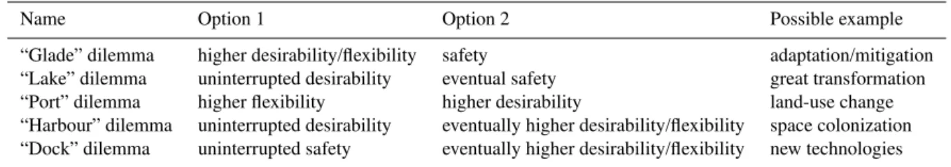
We will see that such questions about a “safe” or “safe and just operating space” (Rockström et al., 2009b; Raworth, 2012; Scheffer et al., 2015; Carpenter et al., 2015) may lead to decision dilemmas that cannot as easily be analysed in a purely optimization-based framework, but that are highly rel-evant for the design of resilient Earth system management strategies. A summary of these dilemmas is contained in Ta-ble 1 (the possiTa-ble examples from Earth system management mentioned there are discussed in the next section).
The paradigm of optimal control, which is much applied in the engineering, on the one hand does not provide suf-ficient concepts for such a qualitative analysis and on the other hand typically requires quite a lot of additional knowl-edge, in particular, some or other form ofquantitative eval-uation of states, e.g. in terms of indicators of human well-being. Of course, the integrated assessment literature, al-though also using optimization as a basic tool, has long real-ized that the spatiotemporal distribution of wealth and the diversity and uncertainty of impacts imply that the prob-lem is hard to frame in terms of a single objective function and has used several techniques to deal with this multi-issue multi-agent decision problem, including certainty-equivalent discount rates and hyperbolic discounting (Dasgupta, 2008), cost–efficiency instead of cost–benefit analyses (Edenhofer et al., 2010), lexicographic preferences (Ayres et al., 2001), and many-objective decision making (Singh et al., 2015), to name only a few, but although qualitative constraints appear in many of them, the actual analyses then typically still focus on quantitative assessments.
In this article, we will complement the above-mentioned set of assessment tools by deriving in a purely topologi-cal way a thorough and precisequalitativeclassification of the possible states of a system with respect to the possibil-ity of avoiding or leaving some given undesired region by means of some given management options. Our results in-dicate that in addition to (or maybe rather before) perform-ing some form of quantitative (constrained) optimization, the sustainable and resilient management of a system may re-quire decisions of a more discrete type, e.g. choosing be-tween eventual safety and permanent desirability, or bebe-tween permanent safety and increasing future options. This appears even more so in the presence of strong nonlinearities, mul-tistable regimes, bifurcations, and tipping elements (Lenton et al., 2008; Schellnhuber, 2009; Keller et al., 2005), where small state changes due to random perturbations or deliberate management may not only have large consequences but can also lead to qualitative and possibly irreversible changes.
To indicate the wide scope of applicability of our con-cepts in various subdisciplines of Earth system science, we illustrate the concepts and dilemmas with conceptual models from climate science, ecology, coevolutionary Earth system modelling, economics, and classical mechanics.
Table 1.Preview of dilemma types discussed in the article.
Name Option 1 Option 2 Possible example
“Glade” dilemma higher desirability/flexibility safety adaptation/mitigation
“Lake” dilemma uninterrupted desirability eventual safety great transformation
“Port” dilemma higher flexibility higher desirability land-use change
“Harbour” dilemma uninterrupted desirability eventually higher desirability/flexibility space colonization
“Dock” dilemma uninterrupted safety eventually higher desirability/flexibility new technologies
physics nature in the sense that they represent the aggregate effects of many micro-scale processes by suitable approxi-mations, their proper interpretation typically requires one to expect small (actually or seemingly) random perturbations. We take this into account here by strengthening the usual no-tion of reachability to one ofstable reachability, and by re-quiring the featured subsets of state space to be topologically open (instead of closed) sets, so that infinitesimal perturba-tions cannot kick the system out of them.
In the next subsection (“Metaphorical framework”), we will briefly summarize our main concepts with the help of a metaphorical illustration, before introducing the correspond-ing formal notation in Sect. 2 in a concise way, reserv-ing a more detailed formal treatment for Appendix A. The framework is then exemplified at the hand of several low-dimensional, conceptual models from various subdisciplines of Earth system science including climate science, ecology, and coevolutionary social–environmental Earth system mod-elling (Sect. 3) in order to indicate the wide scope of appli-cability of our concepts. A thorough analysis of more realis-tic and thus higher-dimensional models of the Earth system is something we have to leave for future studies since that would require further improvement of the numerical meth-ods and algorithms employed for finding region boundaries. We conclude with a discussion and outlook in Sect. 4.
1.1 Metaphorical framework
As a start, let us take the common metaphor that “we’re all in the same boat” literally and represent the state of the Earth system with all its natural and socio-economic parts at each point in time by a single small boat floating or being rowed somewhere on a rather complex system of waters such as in Fig. 1.
The boat can only be on water, not on land, and will gen-erally float along with the stream that represents the inherent dynamics of the Earth system over hundreds and thousands of years (the “default trajectory”), but it may also be rowed in more or less different directions depending on how strong the current of the stream is, and this possibility of rowing rep-resents humankind’s agency in deliberately influencing the Earth system’s course to some extent by some or other form of what we will call “management” below. Let us assume that the main qualitative distinction with regard to where hu-manity wants their boat to be is represented by a division of
Figure 1.Metaphorical summary of concepts introduced in Sect.
1.1 (“Metaphorical framework”) inspired by Schellnhuber (1998). It depicts a river flowing from the mountains to the sea while go-ing through sunny (left) and dark parts (right) where humanity can float and row on a boat. In theshelter, no rowing is needed to
re-main in the sun. One can row against the stream direction in slowly flowing parts, shown with long thin arrows, but in fast parts marked with swirls this is not possible. This setting gives rise to a number of qualitatively different regions of the system’s state space that can be found in any manageable dynamical system as well:upstream
regions such as gladesand lakesfrom where the shelter can be
reached,downstreamregions such as thebackwatersfrom where
the whole region into a desirable, “sunny” region on the left and an undesirable, “dark” region on the right, both contain-ing several parts of the waters that may be connected in any imaginable ways, and with the natural water flow possibly drawing the boat back and forth between these two regions. The sunny region is meant to consist of all those possible states of the natural and socio-economic parts of the Earth system in which some generally agreed environmental and living standards are met, such as those defined by the human rights charter or the sustainable development goals (global goals) recently adopted by the United Nations. An alterna-tive definition of the sunny region has been put forward in the planetary boundary framework (Rockström et al., 2009a; Steffen et al., 2015), where states lying within the corridor of Earth system variability during the Holocene that human societies are adapted to are considered as desirable.
We will show in this article that in such a setting, no mat-ter how the wamat-ters look exactly, the general situation is in a certain sense always equivalent to the situation depicted in Fig. 1. There will in general be a certain sunny water re-gion where one does not need to row at all in order to stay in the sun forever but can simply lean back and let the boat float around inside that region. In the picture, this region is the top-left tranquil tarn, but in general this region may also consist of several disconnected parts which we will call the sheltersto emphasize their desirable and safe nature. Indeed, we will argue below that these shelters may be the most nat-ural candidates for being called a “safe and just operating space for humanity”, only that we may not yet be in them. In the Earth system, there may be several such shelters, one of which might correspond to resilient states of the world (Folke et al., 2010) where humanity lives reconnected to the biosphere (Folke et al., 2011) and no active intervention or constant large-scale management is needed.
Connected to the shelter(s), there will in general also be other parts of the sunny region where it would not be safe to just lean back since the flow would then draw the boat into the dark after some time, but from where the shelters can still be reached by some suitable rowing, as show to the left of the “danger” sign in the image. For their “almost-safe” character, we will call such regions glades. If the glade is for some reason more desirable or offers more flexibility in terms of where one may row, one may face adilemmawhen in a glade, i.e. a qualitative decision problem, namely whether to prefer staying in the safety of the shelter or in the more desirable but unsafe glade.
The shelters may also be reached by rowing from some places within the dark region (e.g. to the right of the “danger” sign) or through such a dark region from some other sunny places (such as those above the “keep out” sign). Among these latter sunny places from where the shelters can be reached only through the dark, there will generally be some places where one may alternatively stay forever in the sun by continuous rowing instead of passing through the dark and leaning back eventually. Such special places as the one
above the “keep out” sign will be calledlakeshere, and they are characterized by a moderate current towards a dark place that one can row against and by the decision dilemma that results from the question of whether one should indeed do so or rather row to a shelter through the dark.
All these regions together will be called theupstream re-gion for reasons that should become clear soon. In any sys-tem’s state space, the upstream consists of all states from which the shelters can be reached by management, and it is partitioned into one or several shelters, glades, dark upstream parts, lakes, and some remaining sunny upstream parts where it is not possible to stay in the sun forever. In Fig. 1, the up-stream ends where therapidsleft of the “keep out” sign be-gin since there the stream becomes so strong that it becomes impossible to row against it in order to eventually reach a shelter. Once the boat has left the upstream via such a rapid, there is no hope of leaning back eventually and staying in the sun, and for this reason the borders of the upstream may be called the “no-regrets planetary boundaries”, forming a middle level of a hierarchy of planetary boundaries we will suggest in Sect. 4.
Further down the stream there will typically be places where it is still possible to stay in the sun forever, only that one has to row over and over again to do so, such as in the slow-moving side branch below the “keep out” sign in the picture. Such regions, calledbackwatershere, are similar to lakes, only without the option of rowing to a shelter, so that the lake dilemma does not occur since the only chance one has is to row against the slow current to stay in the backwa-ter. While the upstream was defined by being able to reach a shelter, thedownstreamis now defined as all places from where a backwater but not a shelter can be reached, includ-ing the backwaters, some dark parts such as the slow-movinclud-ing dark part just right of the backwater in the picture, and maybe some remaining sunny downstream parts from where one may reach a backwater only through the dark. An example of a backwater could be a “machine world” where humanity can fully control nature to its very minute detail. While they can stay within the sunny region for infinite time through this management, there is no way of reaching a shelter anymore because the ecosystem has been changed irreversibly.
dark region from where there is no escape, depicted in the centre of the abyss, will be called atrench.
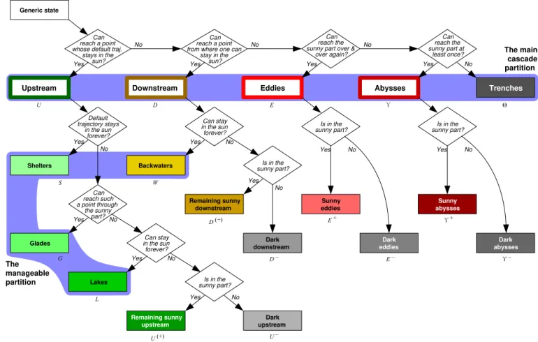
This completes our main partitioning of the Earth system’s or any other manageable system’s state space into qualita-tively different regions: upstream and downstream, defined by being able to reach shelters or backwaters; abysses, de-fined by not being able to avoid ending up in a trench; and eddies in between, defined by being at least able to switch between sun and dark forever. Figure 2 summarizes all these regions in the form of a decision tree, where one can identify the region the system is in by answering a small number of questions. That our partitioning is indeed complete and can be given a suitable and unambiguous mathematical form for all kinds of systems is shown in the next section.
While in Fig. 1, each of the introduced set of system states is just one topologically connected region, in general most of these sets are composed of several disjoint regions, so there may be several shelters, glades, lakes, etc. On a finer level, these may be analysed further by looking at which parts may be reached from which other parts, and this leads to a finer, hierarchical partition intoports, rapids, harbours, docks, etc. and to several new types of dilemmas, as shown in Fig. 3.
All of the five types of dilemmas listed in Table 1 can easily occur in the collective “management” or governance of the Earth system by humanity. A glade dilemma may oc-cur if adaptation is seen as preferable to mitigation for wel-fare reasons but turns out to be a riskier option due to a higher uncertainty of the corresponding climate impacts. A lake dilemma can arise if a great transformation of the global energy system towards a carbon-free economy would tem-porarily lead to welfare losses in poorer countries. A port dilemma may come from the option of increasing welfare by extending industrial agriculture causing biodiversity loss (decreasing flexibility) due to the related large-scale land-use change. A harbour dilemma could occur in the future when colonization of other planets (increasing flexibility) becomes feasible but extremely costly. Finally, a dock dilemma arises whenever a very promising new technology with some un-known risks and side effects (such as genetically engineered food production) could be introduced on a planetary scale.
2 Formal framework
We will now put all of the above on thorough mathematical footing. Let us assume amanageable dynamical system with desirable states, given by the following components:
i. a dynamical system with a state spaceX,default dy-namics represented by a family of default trajecto-ries τx(t), and some basictopologyonX(e.g. the Eu-clidean topology; see Appendix A1 for more detail);
ii. a notion ofdesirable statesrepresented by an open set X+⊆X, called the sunny region, whose complement X−=X−X+we call thedark;
iii. a notion ofmanagement optionsrepresented by a family Mxofadmissible trajectoriesµfor eachx∈X. We assume that one can switch immediately to any trajec-toryµ∈Mx whenever in statex. We say the systemfloats when it follows a default trajectory, and that we mayrowthe system along any other admissible trajectory.
Note that although, formally, we consider deterministic autonomous systems only, non-deterministic systems can be incorporated by considering probability distributions as states, time-delay systems can be treated similarly, and exter-nally driven or otherwise explicitly time-dependent systems can be covered by including timet as a variable witht˙=1 into the state vector. Also, if management involves some form of inertia, e.g. if not the propelling vectorvof a boat
but only its accelerationv˙ can be changed discontinuously, the proper way to model this in our framework would be to treatvas part of the state.
2.1 Qualitative distinction of regions with regard to sustainable manageability of desirability
The main idea of the coarsest of our classifications of states is to first identify (i) asaferegion where management is un-necessary, called the sheltersS, and (ii) a less safe but larger manageable regionMwhere one can permanently avoid the dark at least by management. Then we classify all states with regard to whether and howX+,S, andM can be sta-bly reached from the current state by management. For each state, we ask the following questions. (iii) CanS be stably reached, and if so, can the dark be avoided on the way? (iv) If not, canMbe stably reached? (v) If not, can we stably reach X+over and over again, or at least once again? We will see that these criteria lead to a partition of state space into a “cas-cade” consisting of five main regions: upstream U, down-stream D, eddies E, abysses ϒ, and trenches 2. Each of these will then be split up further into sets such as gladesG, lakes L, and backwaters W by asking further qualitative questions. In choosing these figurative terms, we try to avoid a too technically sounding language and rather extend the useful and common metaphor of “flows” and “basins” in a natural way without trying to match their common-language meanings too accurately.
To acknowledge the fact that all real-world dynamics and management will be subject to at least infinitesimal noise and errors, we base the formal definition of these state space re-gions on certain notions of invariant open kernel, sustain-ability, andstable reachability, whose symbolic mathemat-ical definitions and algebraic properties are detailed in Ap-pendix A2.
2.2 Shelters, manageable region, upstream, and downstream
trajecto-The main cascade partition
Can reach a point whose default traj.
stays in the sun?
Can reach the sunny part over &
over again?
Can reach the sunny part at
least once?
Can stay in the sun forever?
Is in the sunny part?
Is in the sunny part? Default
trajectory stays in the sun
forever?
Is in the sunny part?
Can reach such a point through
the sunny part?
Can stay in the sun forever?
Is in the sunny part?
Can reach a point from where one can
stay in the sun?
Upstream Downstream Eddies Abysses Trenches
Shelters Glades Lakes Remaining sunny upstream Dark upstream Backwaters Remaining sunny downstream Sunny eddies Dark eddies Dark downstream Dark abysses Sunny abysses Generic state The manageable partition
No No No
No No No No Yes Yes Yes Yes Yes Yes Yes Yes Yes Yes No No No No Yes Yes No
U D E ϒ Θ
S W
L G
D (+)
U (+) U –
D – E –
E + ϒ+
ϒ–
b
Figure 2.Decision tree summarizing the partition of a manageable dynamical system’s state space with regard to stable reachability of the
desired region or the shelters (main cascade), and the finer partition of the manageable region. The colour scheme (grey undesired regions, green upstream regions, yellow downstream regions, red eddies, and abysses, with lighter meaning better) is also used in the remaining figures.
ries of all its own points. Thesheltersare the invariant open kernel of the sunny region,
S= X+ι◦
. (1)
S contains all sunny states whose default trajectories stay in the sunny regionX+forever without any management even when infinitesimal (or small enough) perturbations occur. In other words, when insideS, onewill“stably” stay inX+by default.
We call an open setAsustainable(in the basic sense of the word, simply meaning that it can be sustained) iff it contains an admissible trajectory for each of its points. The sustain-able kernel of a setA⊆X, denoted AS, is the largest sus-tainable open subset ofA. We call the sustainable kernel of the sunny region themanageable region:
M= X+S
⊇S. (2)
In other words, when insideM, onecanstably stay inX+by management.
In Appendix A2, we introduce a suitable notion of stable reachability to overcome two problems with the classical no-tion of (plain) reachability known from control theory. For now, let us assume we know what we mean when saying that a stateyor a setY⊆Xisstably reachablefrom some statex throughsome setA⊆X, denotedx Ayorx AY. Using this notion of stable reachability for the choiceA=X(other choices ofAwill be used in the next section), we can now define the upstreamU as the set of states from where the sheltersScan be stably reached at all. Likewise, the down-streamDconsists of all states from which the manageable regionMbut not the shelters can be stably reached:
U=( XS)⊇S, (3)
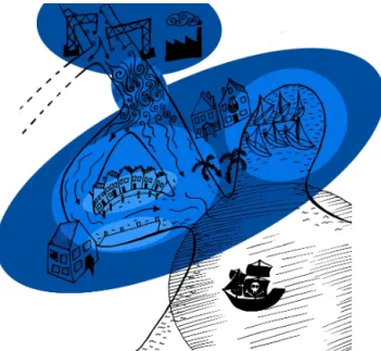
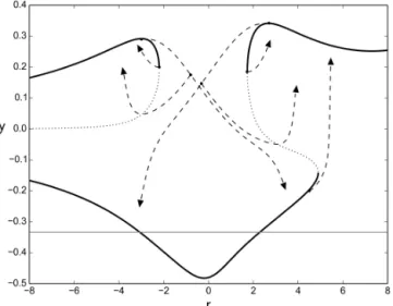
Figure 3.Illustration of port, harbour, and dock dilemmas
intro-duced in Sect. 1.1 (“Metaphorical framework”). As in Fig. 1, hu-manity can float in and row a boat on a complex waterway. From the upperportcity (upper dark-blue region), one can get to some
unknown region to the left and to another, nicer port city (lower dark blue) at the shore through a rapid (hatched blue) which cannot be traversed in the other direction. This choice between desirabil-ity and flexibildesirabil-ity forms a port dilemma. The nicer port city has
two harbours (middle blue regions), of which the right one is more desirable, and between which one can switch only through an unde-sired region where pirates loom (circular area). Boats in the left har-bour face theharbour dilemmaof choosing between either avoiding
the undesired region by all means or eventually reaching a place of higher desirability. Finally, in the left harbour there are two safe
docks(light-blue regions), of which the top one is more desirable,
and between which one can switch only through an unsafe part of the harbour from which one may be drawn into the undesired region if the engine fails. Boats in the bottom dock face thedock dilemma
of choosing between uninterrupted safety and eventual higher de-sirability.
2.3 Trenches, abysses, eddies, and the main cascade On the other, dark end of what we will call the main cascade, we first define the trenches2as that region in the dark from which one cannot stably reach the sunny region even once,
2=X− XX+
(5) (this concept approximately corresponds to the “catastrophe domains” of Schellnhuber, 1998).
Now we turn to the region from where one cannot avoid ending up in the trenches. We define the abysses ϒ as the closure of this region, minus the trenches:
ϒ= {x∈X|∀µ∈Mx∃t>0:µ(t)∈2} −2. (6) The closure is taken since even an infinitesimally small per-turbation from a point in this closure can make the trenches unavoidable.
Finally, the eddiesEare the remainder ofX, i.e. the part from where the manageable region cannot be stably reached but the trenches can be avoided:
E=X−U−D−ϒ−2
=(X−( XM))∩(X−(ϒ+2)). (7) Thus, when in the eddies, even though one can reach the sunny part over and over again, one cannot stay there forever but has to visit the dark repeatedly.
A connected component of2,ϒ, orEwill be called an individual trench, abyss, or eddy, and the latter two typically have sunny and dark parts.
The systemC= {U,D,E,ϒ,2}is a partition ofXwhich we call themain cascade because of the following mutual reachability restrictions:
¬(2 ϒ),¬(ϒ E),¬(E D),¬(D U). (8) In other words, one might at best be able to go in the “down-stream” direction by default or by management, from up-stream to downup-stream to the eddies to the abysses to the trenches, but not in the other, “upstream” direction (see also Fig. 2).
2.4 The glades and lake dilemmas, backwaters, and the manageable partition
Some of the states in the manageable regionM may be in U=( XS) but not in ( X+S). This motivates the definition of two subsets ofMvia the relation of sunny stable reacha-bility, X+, namely (i) the gladesG, from where the shelters can be stably reached through the sun, and (ii) the lakesL, from where the shelters can be stably reached only through the dark:
G=( X+S)−S, (9)
L=M∩U−( X+S)=M∩U−S−G. (10) Glades and lakes are two particularly interesting types of regions since in both one has a qualitative decision prob-lem. Theglade dilemmaoccurs if a glade is for some reason more desirable than its shelter, since then one has to decide whether to stay in the more desirable but unsafe glade or row to the less desirable but safe shelter. Thelake dilemma ex-ists in every lake: shall one stay in the sun by rowing over and over again, but risking to float into the dark if the paddle breaks, or shall one move into a shelter, accepting a tempo-rary passage through the dark, to be able to recline in safety eventually? In other words, the lake dilemma is a choice between uninterrupted desirability and eventual safety. Be-low we will encounter more qualitative dilemmas of this and other types.
rowing over and over again, but where one may not stably reach the shelters at all, not even through the dark:
W =M∩D=M−U. (11)
This completes themanageable partition
M=S+G+L+W. (12)
Also, bothUandDmay contain points outsideM, which we call thedark upstream/downstream,
U−=U∩X−, D−=D∩X−, (13)
and theremaining sunny upstream/downstream,
U(+)= U∩X+
−M, D(+)= D∩X+
−M, (14)
leading to theupstreamanddownstreampartitions
U=S+G+L+U(+)+U−,
D=W+D(+)+D−. (15)
Finally, one can divide the eddies and abysses into sunny and dark parts:
E±=E∩X±, ϒ±=ϒ∩X±. (16)
All the sets introduced so far are summarized in Fig. 2 in the form of a decision tree that allows for a fast classification of individual states.
2.5 Finer distinction of regions with regard to mutual reachability of different types
In addition to the glade and lake dilemmas introduced above, there exist at least three further types of qualitative decision problems, all related to the question of which parts or subre-gions of the above introduced resubre-gions may be stably reached from which other parts, and whether corresponding transi-tion pathways exist that do not leave the shelters or at least the sunny region, or only through the dark. In order to study these questions, we introduce three additional, successively finer partitions derived from the reachability relations X (stable reachability) and X+ (stable reachability through the sun) that we used already above, and from the even more restrictive relation S (stable reachability through the shel-ters).
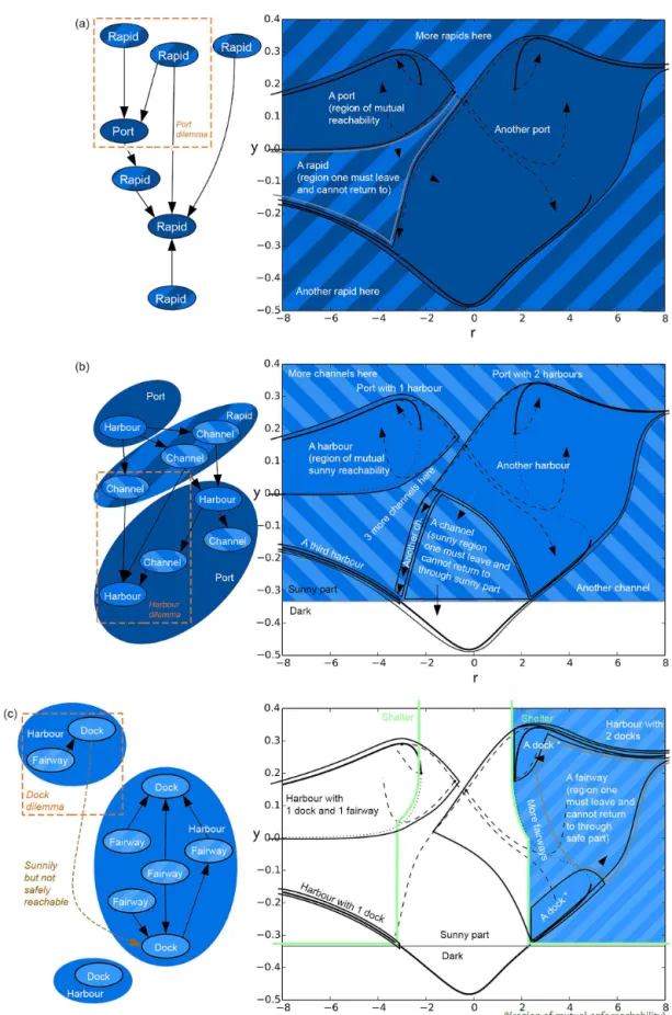
2.5.1 The ports-and-rapids partition and network, and the port dilemma
While from each state inU, one can stably reach some part ofS, one cannot in general navigate freely insideSorUor any other member of the main cascadeC. Let us call a max-imal region in which one can navigate freely aport(see Ap-pendix A3 for more thorough formal definitions and proofs
of the claimed properties). Each port is completely contained in one of the setsU,D,E,ϒ−,2, and none can intersect ϒ+, so the notion of ports fits well into the hierarchy of re-gions that began with the main cascade and the manageable partition. But there are alsotransitionalstates not belonging to any port since one cannot return to them. Thus, to extend the system of all ports into a partition of all ofX, we also have to classify these non-port states, and we do so by ask-ing which ports they can reach and from which ports they can be reached. States that are equivalent in this sense form what we call arapid. It turns out thatUandDare then par-titioned into ports and rapids, and so is each individual eddy, abyss, and trench. The reachability relations between ports and rapids form a directed network that concisely summa-rizes the overall structure of all management options.
Figure 1 shows the very simple case of a linear network: the whole upstream is one port, the sunny downstream and the adjacent fast-moving part of the dark downstream form a rapid, the backwater and the slow-moving part of the dark downstream form another port, the waterfall is another rapid, the eddy is a port again, and the abyss and the trench are rapids. In the examples below, we will, however, see that much more complex ports-and-rapids networks may occur in models, and one can prove that any acyclic graph may occur as the ports-and-rapids network of some system.
The ports-and-rapids partition is helpful in the discussion of a certain type of dilemma that results from two different objectives which may not be easily balanced: (i) the objective of being in or reaching a state with highintrinsic desirability, e.g. as measured by some qualitative preference relation finer than the mere distinction between “desirable” and “undesir-able”, or even by some quantitative evaluation such as a wel-fare function, and (ii) the objective of retaining an amount of flexibilityas large as possible by being in or reaching a state from which a large part of state space is reachable. Flexi-bility may be important in particular in situations in which there is some uncertainty about future management options and/or future preferences (Kreps, 1979). We call this aport dilemma.
2.5.2 The harbours-and-channels partition and network, and the harbour dilemma
Since they do not take into account the definition of the desir-able regionX+at all, ports and rapids are not directly com-patible with the regions from the manageable partitionM since their members may overlap in complex ways. However, we can construct a very similar but finer partition based on stable reachability through the sun ( X+) instead of (plain) stable reachability, restricted to the sunny region, and the re-sult turns out to be compatible withM.
reached from the same harbours through the sun is called a channel. Since each harbour or channel lies completely in a port or a rapid, the harbours and channels form a finer par-tition than the ports and rapids and form a finer layer of the reachability network in which the links represent reachability through the sun instead of mere reachability.
The harbours-and-channels partition allows one to identify decision problems involving (i) the objective ofstayingin a desirable state and (ii) the objective of eventuallyreachinga state with higher desirability or flexibility, which is called a harbour dilemmahere.
2.5.3 The docks-and-fairways partition and network, and the dock dilemma
Note that although the harbours-and-channels partition is finer than that into ports and rapids, there is still one impor-tant region that can have nontrivial overlaps with harbours and channels, namely the sheltersS. In order to complete our hierarchy of partitions and networks of regions, we there-fore introduce a third and finest partition and network level, restricted to S, based on the notion of stable reachability through the shelters, S.
In complete analogy to the above, a maximal region of states that are mutually reachable throughSis called adock, and the non-dock states inSare classified into so-called fair-wayswith regard to their reachability of these docks. Again, each dock or fairway lies completely in a harbour or channel, and they form a third layer of the reachability network whose links now represent the safest form of reachability, namely through the shelters.
Finally, the docks-and-fairways partition is helpful in the discussion of dilemmas involving (i) the objective of staying in asafe state (i.e. in the shelters) and (ii) the objective of eventually reaching a state with higher desirability or flexi-bility. We call this adock dilemma.
2.6 Summary of the introduced hierarchy of partitions and networks
To summarize, we have now a hierarchy of ever-finer parti-tions of the system’s state space at our hands. We began with the main cascadeC= {U,D,E,ϒ,2}, its refinement into the partition {S,G, L,U(+),U−,W,D(+),D−,E+,E−, ϒ+,ϒ−,2}(see Fig. 2), and the further refinement by topo-logical connectedness into individual shelters, glades, lakes, backwaters, eddies, abysses, and trenches. These partitions represent the qualitative differences in stable reachability of the shelters or the manageable set, thus allowing for a first classification of states with regard to the possibilities of sus-tainable management, and may reveal decision problems of the type of glade or lake dilemma which will occur in many of the examples below, where one has to choose between higher safety and higher desirability or flexibility or between uninterrupted desirability and eventual safety.
A different refinement ofC into the ports-and-rapids net-work is still based on stable reachability alone but contains other details suitable for the identification and discussion of possible port dilemmas that involve a choice between higher desirability and higher flexibility. Inside the desirable regionX+, this partition can be refined into the harbours-and-channels network suitable for the discussion of harbour dilemmas that involve a choice between uninterrupted desir-ability and eventually higher desirdesir-ability or flexibility, and further into the docks-and-fairways network suitable for the discussion of dock dilemmas that involve a choice between uninterrupted safety and eventually higher desirability or flexibility (Table 1).
These three networks may also be interpreted as a three-level “network of networks” with nodes representing state space regions of different quality and size. A network-theoretic analysis of it using methods such as the node-weighted measures of Heitzig et al. (2012) may especially be interesting in the context of varying system parameters and bifurcations such as those in Fig. B2, but this is beyond the scope of this article.
3 Examples
In this section, we will apply the introduced framework to several illustrative examples from natural and coevolutionary Earth system modelling, ecology, socio-economics, and clas-sical mechanics. The examples have been chosen not for their realism but for their simplicity in order to show the broad scope of potential applicability of our concepts, as well as the relevance of the identified types of decision dilemmas in both the natural and socio-economic components of the Earth system.
3.1 Carbon cycle and planetary boundaries
Our first example is from natural Earth system modelling and illustrates which of the above-introduced regions occur most often for systems that possess only a single, globally stable, and desirable attractor.
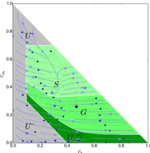
Anderies et al. (2013) proposed a conceptual model of the global carbon cycle capturing its main features while keeping the model sufficiently low-dimensional to be able to discuss the planetary boundaries concept with it. We use their model for pre-industrial times, which has three dynamical variables cm,ctandca=1−cm−ctrepresenting the maritime, terres-trial, and atmospheric shares of the fixed global carbon stock. The dynamics are of the form
˙
cm=am(ca−βcm), c˙t=f(ca, ct)−αct,
Since the parameterα can be considered the natural hu-man hu-management option for this system, we assume the de-fault flow has a value of α=α+=0.5, while management can reduce it by half toα=α−=0.25, which results in the trajectories shown in Fig. 4. Both have a unique stable fixed point in the interior of the state space which is globally at-tractive for all states withct>0.
In order to roughly represent the planetary boundaries re-lating to climate change, biosphere integrity, and ocean acid-ification (Rockström et al., 2009b; Steffen et al., 2015), we require a “sunny” state to have sufficiently low atmospheric carbon, at least a minimum value of terrestrial carbon, and not too large maritime carbon, leading to a dark region of the shape shown in Fig. 4 in grey. If, as shown, the unmanaged fixed point is sunny, one obtains a purely upstream situation with a shelter surrounding the fixed point, a glade, and a re-maining sunny upstream U(+) as shown in the figure. For our (quite arbitrarily) chosen parameter values, a trajectory starting in the sunny upstream is likely to first cross the cli-mate boundary and then the biosphere boundary before get-ting back into the sunny region, whereas it seems quite un-likely to cross the acidification boundary.
In this example, all non-upstream regions are empty, and so is the lake region; hence, no lake dilemma occurs. On the other hand, if one considers a higherctto be preferable, we get an example of the glade dilemma since the managed fixed point in the less safe glade has higherctthan the unmanaged fixed point in the safer shelter. Note that this is neither a port, harbour, or dock dilemma since both points are in the same port and harbour and only the unmanaged one is in a dock.
If, instead, we had chosen the minimum value for ct to be larger than the unmanaged equilibrium value, the shelter would be empty and the whole situation would change from upstream-only to either a downstream-only or an abyss-and-trench situation. This type oftopological bifurcationwill be studied in Sect. 3.4. In the next example, we will see a lake dilemma instead of a glade dilemma.
3.2 Competing plant types and multistability
The second example, from ecology, demonstrates how the lake dilemma may occur in a multistable system with a sunny and a dark attractor.
In this fictitious example, two plant types (1 and 2) com-pete for some fixed patch of land, modify the soil, and are harvested. Their growth follows logistic-type dynamics, with land cover proportionsx1,2∈[0, 1] following the equations
˙
x1=x1 K1 x1,2−x1−h1x1, ˙
x2=rx2(K2(x1,2)−x2)−h2x2.
In this, r >1 is a constant productivity quotient, h1,2 are the harvest rates, and the two dynamic capacities K1(x1,2)=√x1(1−x2)61 andK2(x1,2)=√x2(1−x1)61
represent the fact that each type modifies the soil quickly
Figure 4.Phase portrait of the pre-industrial carbon cycle model
of Anderies et al. (2013). Arrows indicate default/unmanaged dy-namics (pale blue) and alternative/managed dydy-namics (dotted dark blue) from reducing the human offtake rate by half. Filled dots: cor-responding stable fixed points. Grey area: undesired region defined by (i) upper bounds for maritime carboncm(white horizontal line,
representing a planetary boundary related to ocean acidification) and atmospheric carbon 1−ct−cm(white diagonal line, related to
a climate change boundary) and a lower bound for terrestrial carbon
ct(white vertical line, representing an ecosystem services planetary
boundary). Coloured areas and labels: derived state space partition (see text); colours as defined in Fig. 2: a shelterSaround the
glob-ally stable fixed point of the default dynamics, a gladeGfrom where Scan be reached by management without violating the bounds, and
a remaining sunny upstreamU(+)from where one cannot avoid
vi-olating the bounds temporarily.
to its own benefit but to the other type’s disadvantage (see Supplement 1 for a discussion of the model design based on Bever (2003), Kourtev et al. (2002), Kulmatiski et al. (2011), Levine et al. (2006), Poon (2011), and Read et al. (2003).
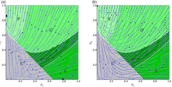
Figure 5.Competing plant types example, showing all upstream regions and illustrating the lake dilemma. A bistable system of two
com-peting plant types with two simultaneous management options (depicted in separate plots only for discernibility). Management by a general harvesting quota (dotted arrows shown left) can ensure desirable long-term harvests of the less productive typex1(lakeL). Management
by temporary protection of the more productive typex2(dashed arrows shown right) can cause a transition to the desirable fixed point (in
theshelterS), but only through the undesired region of low harvests (grey region). The state space partition boundaries resulting from both
options together (white curves) and a desirable minimum harvest boundary (white diagonal) follow some admissible trajectory at each point.
set the desirable region to wherex1+x2> ℓfor someℓ >0 in order to ensure some minimum harvests.
For the choicer=2,h+=0.2, h−=0.1, ℓ=0.65 of the figure, the desirable high-productivity stable fixed point of the default dynamics at≈(0, 0.79) is in the sunny region and is thus contained in a shelterS. The latter is delimited by the default trajectory that meets the boundary to the undesired re-gion tangentially.Scan be stably reached from all states with x2>0, and hence the upstream isU= {(x1,x2)|x2>0}. The border of the gladeGnext toScan be found by backtracking the “widest” admissible trajectory that meets the boundary to the undesired region tangentially; this turns out to be a type 2 management trajectory as seen in Fig. 5 (right panel). This shows how the boundaries of regions may often be found by identifying tangential or otherwise significant points and backtracking the default and alternative trajectories leading to them.
The lower-productivity stable fixed point of the default dy-namics (withh1,2=h+) at≈(0.52, 0) is undesired for this choice ofX+. From it one cannot only navigate toSbut can also (and faster) get to the higher productivity stable fixed point of the first type ofmanageddynamics withh1,2=h−, at≈(0, 0.79), and stay there as long as management holds. Hence the region around (0, 0.79) is part of the manageable region M. The exact boundary of this region (which soon turns out to be a lake,L) is the “widest” admissible trajectory that meets the boundary to the undesired region tangentially; in this case, this trajectory turns out to be a type 1 manage-ment trajectory as seen in Fig. 5 (left panel). To get from this type 1-dominated region to the type 2-dominated
shel-terSvia the other management option of protecting type 2, one has to cross the undesired middle region in which both types coexist at a low level due to soil conditions that are suboptimal for both types. Hence the region around (0, 0.79) is a lake. The associated lake dilemma is similar to a glade dilemma in that staying in a lake is unsafe as in a glade, but it differs in the reason why one may want to stay there: while staying in a glade may be attractive simply because the glade may be more desirable than the shelter in some quantitative sense, staying in a lake may seem attractive since that avoids having to pass through the dark to reach safety.
This form of the lake dilemma can also occur in other mul-tistable systems when one of the attractors is in the dark but sufficiently close to the sunny region so that constant man-agement can sustain the system in a sunny place near that attractor, and when other management options may push the system towards another, sunny attractor after crossing the dark.
0.0 0.2 0.4 0.6 0.8 1.0 z1=0.3 +xx1 1
0.0 0.2 0.4 0.6 0.8 1.0
z2
=
x2
0.
3
+
x2
S
U−
Θ U( +)
G
Υ+
Figure 6. Substitution of a dirty technology. Coevolution of the
cumulative production of a dirty technology (x1) and a clean one
(x2) without (pale-blue curves) and with (dotted dark-blue curves)
a subsidy for the clean technology. Undesired region with too high future usage of the dirty technology coloured in grey. Knowledge stocksx1,2were transformed toz1,2=x1,2/(0.3+x1,2) in order to
capture their divergence to+∞.
The example also shows that the more management op-tions exist, the less trivial it is to find the boundaries be-tween regions even in two-dimensional systems. For higher dimensions, one will usually have to rely on specialized nu-merical algorithms such as the viability kernel algorithm of Frankowska and Quincampoix (1990) from viability theory.
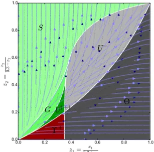
3.3 Substitution of a dirty technology
Our third example concerns a purely socio-economic part of the Earth system that bears some similarity to the preced-ing example but features regions from both ends of the main cascade: upstream and abyss/trench, without having the in-termediate regions of downstream and eddies.
Instead of plants, in this example a certain produced good (e.g. electric energy) comes in two types which are econom-ically perfectly substitutable but whose production processes use two different technologies – one “dirty” and one “clean” (e.g. conventional and renewable energy). The production costsC1andC2are convex functions of production output per timeyiand decrease over time via learning-by-doing dy-namics that are similar to Wright’s law (Nagy et al., 2013):
Ci(yi)=γiyi1+σi/(1+σi)xiαi.
In this,xiis cumulative past production (withx˙i=yi),γi are cost factors,σi>0 are convexity parameters, andαi>0 are learning exponents. We assume that demandDdepends lin-early on price, D(p)=D0−δp,δ >0; that demand equals
production,D=y1+y2(“market clearance”); and that price equals marginal costs,p=∂C/∂yi=γiyiσi/xiαi, due to per-fect competition among producers. One can then uniquely solve for the produced amounts yi, getting some formula yi=fi(x1,x2). This results in a two-dimensional dynamical system with state variablesx1,x2and equations
˙
xi=fi(x1, x2).
Let us putD0=1,δ=1,σi≡1/5,αi≡1/2, and assume that the default dynamics haveγi≡1, so that the long-term default behaviour is p(t)→0, D(t)→1. If the dirty tech-nology (1) is the traditional one, so thatx1(0)> x2(0), we havex1(t)→ ∞,x2(t)→ ˆx2<∞,y1(t)→1, andy2(t)→0, i.e. usage of the clean technology (2) will die out. If instead x1(0)< x2(0), technology 1 will die out. Hence the system is bistable as in the plant example, but with attractors at infin-ity. To depict the diverging behaviour, we used the transfor-mationzi=xi/(0.3+xi) in Fig. 6.
The main dynamical difference to the plant example is, however, not the diverging behaviour, but has to do with the choice of management options. While in the plant example, the choice of management options led to an upstream-only situation in which the more desirable fixed point could be reached from everywhere, in this example we will get regions from which the desirable fixed point cannot be reached and which are thus non-upstream. We consider the management option of lowering γ2 to a value of, say, 1/2 by subsidis-ing the clean technology to induce a technological change (Jaffe et al., 2002; Kalkuhl et al., 2012). This leads to the al-ternative dynamics depicted in Fig. 6, showing that for some initial states withx1> x2one can now getx2(t)→ ∞ and y1(t)→0. The goal of keeping the usage of the dirty technol-ogy below some limit,y1< ℓ <1, corresponds to a desirable region in terms ofx1,x2, whose border can be computed as x2=x1(1/ℓ−1−1/ℓ4/5√x1)2/5 (see Fig. 6). That goal is automatically fulfilled in the top-left shelter region, can also be sustained by management (subsidies) in the glade region below it, and can at least be reached eventually from the re-maining sunny upstreamU(+)below the glade and from the dark upstreamU−, which is delimited by the management trajectory that meets the upper right corner.
But from below the latter trajectory, the shelter cannot be reached. In other words, when inU−, one has to act fast in order not to lose the option of reaching S. From the dark part denoted2, not even the sunny region is reached, and hence that region is a trench, while the sunny part to its left is the abyss leading to that trench. There are no intermediate regions (downstream or eddies) between upstream and abyss in this example.
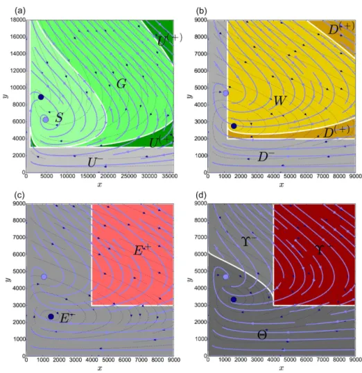
Figure 7. Combined population and resource dynamics. Coevolution of a population x and a resource stock y. In all cases, φ=4, r=0.04. When the globally stable fixed point of the default dynamics (pale blue) falls intoX+, only upstream regions occur (top-left
panel, γ0=4×10⁻⁶> γ1=2.8×10⁻⁶, δ= −0.1,κ=12 000, xmin=1000, ymin=3000). When it falls into X− instead, but the
sta-ble fixed point of the alternative management trajectory (dotted dark blue) is in X+, then only downstream regions occur (top-right
panel,γ0=8×10⁻⁶< γ
1=13.6×10⁻⁶,δ= −0.15,κ=6000,xmin=1200,ymin=2000). Otherwise (bottom panels,γ0=8×10⁻⁶< γ 1, δ= −0.15,κ=6000,xmin=4000,ymin=3000), the analysis depends on whether one can repeatedly reachX+by switching between
de-fault and alternative trajectories: forγ1=16×10−6(bottom-left panel), only eddies occur, while forγ
1=11.2×10⁻⁶(bottom-right panel),
only abysses and trenches occur.
coupled with a socio-economic Earth system component and shows how different parameters may qualitatively move the resulting state space topology through the whole main cas-cade, from an upstream-only situation via downstream-only and eddies-only to an abyss-and-trench situation.
The model was used in Brander and Taylor (1998) to ex-plain the rise and fall of the native civilization on Rapa Nui (Easter Island) before western contact, but it may also be interpreted as a conceptual model of global population– vegetation interactions. It is derived from simple economic principles and leads to a modified Lotka–Volterra model with a finite resource. The human populationx is preying on the island’s forest stocky, which itself follows logistic growth dynamics:
˙
x=δx+φγ xy, y˙=ry(1−y/κ)−γ xy
for some parametersγ,δ,κ,φ, andr representing growth and harvest rates and the stock’s capacity.
We assume management will either reduce the default har-vest rateγ0 to some smaller value γ1< γ0 to avoid over-exploitation of the resource or increase it to a larger value γ1> γ0to avoid famine. Our choice of the sunny region re-lies on two principles. The absolute population should not drop below a thresholdxminand the relative decline in popu-lation under the default dynamics,− ˙x/x, should not exceed a value ofℓ. HenceX+= {x > xmin andy > ymin=max(0, −(ℓ+δ)/φ γ0)}.
Figure 8. Gravity pendulum fun ride with management by
one-sided acceleration and undesirable fast rotations. The 2π-periodic
coordinateθ is the pendulum’s inclination angle. If its angular
ve-locityωexceeds±ℓ, people get sick (grey region). Since staying in L(balancing almost upright) orG(balancing somewhat inclined) is
more exciting than inS(resting downward), we have both a glade
and a lake dilemma.
managed fixed points belong to the desired or undesired re-gion. In Appendix B2, these kinds of transitions are more formally interpreted as bifurcations.
An interesting case occurs when the whole state space is a single eddy as in Fig. 7 (bottom-left panel): one can then re-peatedly visit the sunny region by suitably switching between a low default harvest rate and a managed higher harvest rate, but one cannot avoid getting back into the undesired region of a low or fast declining population. An “optimal” manage-ment strategy would then lead to slowly but strongly oscillat-ing behaviour.
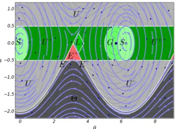
3.5 Gravity pendulum fun ride
While in the above examples typically only some of the pos-sible regions were non-empty for each parameter combina-tion, the following example from classical mechanics dis-plays a rich diversity of state space regions that coexist at a single choice of parameter values. Despite extremely sim-ple dynamics, it features both a glade and a lake dilemma, an eddy, and a trench at the same time.
In the model, people sit in a fun ride resembling a gravity pendulum with angle θ and angular velocityω and default dynamics given by
˙
θ=ω, ω˙ = −sinθ.
An optional additional clockwise acceleration of the pendu-lum of magnitudea >0 (“management”) leads to alternative admissible trajectories on which for some time interval(s) one hasω˙= −sinθ−a. The sunny region is where|ω|< ℓ, for someℓ >0 representing a safety speed limit above which people might get sick.
The unique shelterSis delimited by the default trajectory leading through the pointsθ=2kπ,ω= ±ℓthat surrounds the stable resting state ofθ=ω=0 (see Fig. 8). If a state lies on a default trajectory that hasω >0 (anticlockwise pendu-lum motion) at least some of the time, then there is an ad-missible trajectory from it leading into the shelter, generated by the management strategy of “braking” wheneverω >0. Hence the upstreamUequals the region strictly above the de-fault trajectory withω <0 that connects the unstable saddle point atθ=(2k+1)π,ω=0 (pendulum balancing upright) with itself.
Just left of the shelter is the unique gladeG. Depending on the parameter values, the stable fixed point of the managed dynamics (hanging pendulum inclined by constant acceler-ation) may either belong to the shelter or to the glade. In the latter case (Fig. 8), we have a glade dilemma since the inclined position is preferred to the resting position by the riders but is unsafe since if the engine breaks, people will get sick.
An even more exciting position is close to the upright bal-ancing saddle point, atθ slightly larger than (2k+1)π and ω≪1, where there is an admissible trajectory that stays close to there (by braking repeatedly for short intervals while stay-ing almost upright), so that this point is in the manageable regionM. This is a typical example of how a region close to a saddle point of the default dynamics may become man-ageable due to an alternative feasible trajectory that has a slightlyshifted saddle point, so that in the diamond-shaped region between the two saddle points, one can concatenate unmanaged and managed trajectories into periodic orbits.
However, for choices such asa=0.6 andℓ=0.5 (Fig. 8), there is no admissible trajectory leading from the exciting region with θ≈(2k+1)π, ω≈0 into the shelter without entering the region with|ω|> ℓ. In that case the diamond-shaped region is a lake and we have a lake dilemma.
Finally, the region below and including the default trajec-tory that touches the lineω= −ℓfrom below is the trenches since one cannot brake in that direction, and the region be-tween the trench and the upstream is the eddies. Downstream and abysses are empty in this example.
3.6 Bifurcations with manageable parameter
This final example system is designed to illustrate the rela-tionship of reachability and bifurcations of a dynamical sys-tem that can be managed through a parameter and shows bi-furcations of the type typically associated with tipping ele-ments of the Earth system (Schellnhuber, 2009).
It has a two-dimensional state spaceX= {(r,y)}, where the “fast” variabley∈Rhas default dynamics
˙
y=h(y|r)= −4+r23y3+2r2−1 4+r2y+er−10,
Figure 9. Bifurcations with manageable parameter. Loci of
sta-ble (solid black lines) and unstasta-ble (dotted lines) fixed points ofy˙= −(4+r2)3y3+(2r2−1)(4+r2)y+er−10. Leftmost and rightmost admissible management trajectories (dashed arrows) and their starting points (dots). Border (grey line) between sunny region
y >−1/3 and the dark. See Fig. 10 for an analysis.
which, however, can be changed by management up to a velocity at most 100 and with arbitrarily large acceleration, leading to admissible trajectories with r˙∈[−100, 100] and
˙
y=h(y|r). We assume that values ofy6−1/3 are undesir-able.
If r is instead interpreted as a parameter of the one-dimensional systemy˙=h(y|r), the setXcan be interpreted as its bifurcation space in which one can plot a bifurcation di-agram consisting of the loci of stable (solid lines) and unsta-ble (dotted lines) fixed points, as shown in Fig. 9. As one can see, there are three saddle-node bifurcations at r1≈ −2.2, r2≈1.735, andr3≈4.9 with monostable parameter regimes r1< r < r2andr > r3, and bistable parameter regimesr < r1 andr2< r < r3. Individual and paired saddle-node bifurca-tions (which often result from fold bifurcabifurca-tions) occur fre-quently in bistable Earth system components such as the hys-teretic thermohaline circulation (Stommel, 1961; Rahmstorf et al., 2005), monsoonal soil–vegetation feedbacks (Janssen et al., 2008), or other tipping elements (Schellnhuber, 2009). Hysteresis also occurs on other spatial and temporal scales, e.g. in local hydrology (Beven, 2006) and in long-term glacial climate dynamics (Ganopolski and Rahmstorf, 2001). The main part of the resulting network of ports and rapids of our example system is depicted in Fig. 10. On its coars-est level, there are two ports, each containing one of the two connected loci of stable/unstable fixed points, and a rapid in between through which one can pass from the left to the right port but not back. If the right port seems more attractive, e.g. because it allows a higher value of y, we have a port dilemma since by leaving the left port for the right one, we lose flexibility in terms of reachable regions.
The right port contains two harbours, similarly connected by a narrow “internal” channel, as well as another “exit” channel leading from the right harbour to the dark region. Note that on the leftward-pointing dashed management tra-jectory in the middle of the bifurcation diagram, there is a leftmost point from where one can still “turn around” and reach (if only unstably) the right part without entering the dark region; this point is a corner of the right harbour (but not belonging to it, for stability reasons), and below it is a chan-nel leading to another harbour in the bottom left. Again, if the right harbour seems more attractive, we have a dilemma, this time a harbour dilemma, since in order to reach the right harbour from the left one, we have to pass through the dark.
Finally, the right harbour contains two docks again con-nected by a fairway, plus some more fairways. Again, we get a dilemma if the top-right dock is more attractive than the top-left one: the dock dilemma is that, in order to reach the top-right dock from the top-left one, one has to pass through the unsafe middle region and risk ending up in the dark if management breaks down.
4 Discussion and conclusions
We have presented a formal classification of the possible states of a dynamical system such as the Earth system into re-gions of state space which differ qualitatively in their safety, the possibilities of reaching a safe state, the possibilities of avoiding undesired states, and in the amount of flexibility for future management.
Figure 10.Main part of the three-level reachability network of ports and rapids (top panel), harbours and channels (middle panel), and
ups and downs. It must remain an open question here whether this effect might be an additional explanation for empirically observable cycles such as business or resource cycles when management is involved.
The introduced concepts have then been used to point out a number of qualitatively different decision problems: the glade, lake, port, harbour, and dock dilemmas. In our opin-ion, one particularly nasty form of decision problem is the lake dilemma, where one has to choose between uninter-rupted desirability and eventual safety, and Sect. 3.2 indicates that this dilemma may easily occur at least in ecological sys-tems or other multistable syssys-tems with a sunny attractor and another one slightly in the dark. Since the transformation of socio-metabolic processes or complex industrial production systems may resemble the soil transformation of Sect. 3.2, one may also expect the lake dilemma to occur in the socio-metabolic and economic subsystems of the Earth, e.g. in the context of a great transformation leading to decarbonisation of the world’s energy system. The form of lake seen near the saddle point in the pendulum (Sect. 3.5) can also occur in other nonlinear oscillators, e.g. the Duffing oscillator or mod-els of glacial cycles that resemble it such as Saltzman et al. (1982) and Nicolis (1987), when a management option exists that has a slightly shifted saddle point. This indicates that the lake dilemma may also occur in purely physical subsystems of the Earth system.
We argue that our concepts may be especially useful in the context of the current debate about planetary bound-aries (PBs), a possible safe and just operating space (SAJOS) for humanity, and the necessary socio-economic transitions to reach it or stay in it. We suggest that the region delimited by some identified set of PBs in the sense of Rockström et al. (2009a) and Steffen et al. (2015) and some similar socio-economic limits, e.g. those relating to the United Nations sus-tainable development goals (Raworth, 2012), should be inter-preted in our framework as a natural choice for the desirable region X+, although their definitions already contain some reasoning about the consequences for the respective sub-systems when the boundaries are violated. Such boundaries might be called the ultimate planetary boundaries (UPBs), and they are typically defined by some simple thresholds for relevant indicators as in Rockström et al. (2009a) and Stef-fen et al. (2015), not taking into account theoverallsystem’s inherent dynamics much. In this sense, UPBs are typically “non-interacting”. Based on the UPBs, one may then try to identify one or more smaller shelter regions S that can be considered a SAJOS in the sense that, once there, no further large-scale management in the form of global policies is nec-essary to stay within the limits for all times (or at least for a sufficiently long planning horizon). The borders of these shelters are also a form of PBs but are much more restrictive than the UPBs we started with, and we suggest to call them safe planetary boundaries (SPBs).
If it turns out that the current state of the Earth is out-side the shelters, one should then aim next at trying to decide
whether it is in the upstream. If so, knowledge about whether it is in a glade or lake or not, and which safe docks can be stably reached, will be necessary in order to choose a man-agement path. In the glade case, one can still reach the shelter without ever violating the UPBs by appropriate management; hence we suggest to refer to the border of shelters and glades together as the provident planetary boundaries (PPBs).
In the lake case, one has to decide instead whether a tem-porary violation of the UPBs can be justified by the eventual safety of the shelters. In addition, a port dilemma may ne-cessitate a decision between higher desirability and higher flexibility at this point. Only after these qualitative decisions have been made does it seem advisable to optimize the cho-sen type of management pathway by means of more tradi-tional control and optimization theory, hopefully using ac-curate enough quantitative estimates of the involved options, costs, and benefits. Once in the shelters, one may start car-ing about improvcar-ing the state further by movcar-ing between docks to either improve desirability or flexibility, but this may require a risky temporary passage through a sunny but unsafe region (which poses a dock dilemma) or even a pas-sage trough the dark (which poses a harbour dilemma). Of course, many combinations of these qualitative and quantita-tive criteria may appear in the actual global decision process, e.g. in the form of lexicographic preferences, decision trees, or more sophisticated welfare measures or other quantitative objective functions that take the topology suitably into ac-count and that may relate to some form of market (or other game-theoretic) equilibrium or else be governed by some suitable policy instruments, as kindly suggested by an anony-mous referee.
If we are not in the “upstream” of the Earth system, prospects are worse. Violating the limits can then only be avoided by management, either eventually forever (if in the downstream), or only repeatedly but with repeated violations occurring (if in the eddies), or even only for a limited time with an ultimate descent into the undesired region (if in the abysses or already in the trench). We suggest to call the up-stream borders the no-regrets planetary boundaries (NRPBs). If the diagnosis reads “eddy”, “abyss”, or “trench”, one may repeat the analysis with a less ambitious, “second best” definition of the desirable region by choosing less restrictive UPBs, or revert to quantitative optimization, e.g. to mini-mize some damage function along the system’s trajectory. On the other hand, as long as one is in the “manageable re-gion”M(shelters, glades, lakes, and backwaters), the UPBs need never be transgressed if managed wisely; hence we propose to call the borders ofM the foresighted planetary boundaries (FPBs).