CROSS
Monte Carlo Simulation and Cross-Entropy
João Meneses Figueiredo Costa
F
INALV
ERSIONDissertation submitted in fulfillment of the requirements
for the Master in
Electrical
and Computers Engineering
in the
Major
of Energy
Supervisor
: Vladimiro Henrique Barrosa Pinto de Miranda (
Ph.D.)
Co-
supervisor: Leonel de Magalhães Carvalho (
Ph.D.)
i
Abstract
The planning of power system operations is a complex problem, mostly due to the presence of uncertainties tied to the multiple variables of such system. Given the liberalization of the power systems in late 20th century, early 21st century, and its continued evolution as well
as the expanding accessibility of the transmission and distribution networks provided to the distributors and the consumers with the introduction of micro-production and renewable energy options, this planning problem grows in complexity at an exponential rate.
Initially treating these problems and modelling them based in probabilistic concepts, presented a problem due to the lack of data related to the behavior of each variable. The Sequential Monte Carlo simulation (MCS) method is one of the most powerful tools for power systems reliability assessment.
Through sequentially sampling the durations of the different states for the multiple components that compose the power systems, this method can somehow simulate the stochastic behavior of such components. Therefore, time-dependent issues like the renewable power production, micro-grid operation, scheduled maintenance, hydric thermal power systems, the evolution of the system load, etc.
Presenting itself with numerous advantages, such as making it possible to estimate average durations for different events and their frequency, as well as quantify the power unavailability associated with each system failure. The MCS major downside is the simulation time, sometimes too slow due to computational effort of the method itself.
As so the main objectives of this dissertation are to investigate alternative and incorporated methods based on the Cross-Entropy theory and propose algorithmic advances that can effectively improve the time-efficiency of the sequential MCS simulation.
iii
Resumo
O planeamento das operações do sistema de energia é um problema complexo, principalmente devido à presença de incertezas ligadas às múltiplas variáveis do referido sistema. Dada a liberalização dos sistemas de energia no final do século 20, início do século 21, e sua evolução contínua, bem como a acessibilidade a expansão das redes de transmissão e distribuição dadas aos distribuidores e os consumidores, com a introdução de microprodução e opções de energia renovável, este problema de planeamento cresce em complexidade a uma taxa exponencial.
Inicialmente, o tratamento destes problemas e modelização baseada em conceitos de probabilidade, apresentou um problema devido à falta de dados relacionados com o comportamento de cada variável. O método de simulação Monte Carlo Sequencial (MCS) é uma das ferramentas mais poderosas para avaliação da fiabilidade de sistemas de energia, através da sequencial amostragem as durações das diferentes estados para os vários componentes que compõem os sistemas de energia, este método pode de alguma forma simular o comportamento estocástico dos ditos componentes, os mesmos problemas dependentes do tempo, como a produção de energia renovável, a operação micro-rede, manutenção programada, os sistemas de energia hídrico-térmicos, a evolução da carga do sistema, etc.
Apresentando-se com inúmeras vantagens, como tornando-se possível estimar durações médias para diferentes eventos e sua frequência, bem como quantificar a indisponibilidade de energia associada a cada falha do sistema, a principal desvantagem MCS é o tempo de simulação, por vezes demasiado lento devido ao esforço computacional do próprio método.
Como assim os principais objetivos desta tese são, investigar métodos alternativos incorporados com base na teoria entropia cruzada e propor avanços algorítmicos que possam melhorar eficazmente o tempo-eficiência da simulação MCS sequencial.
v First of all, I’d like to talk about my supervisor, Professor Doctor Vladimiro Henrique Barrosa Pinto de Miranda, who I met in my 4rd year o MIEEC and have learned a lot from him the last two years, and when the opportunity arose to work together, I didn’t think twice. I’d like to express my sincere gratitude, for a major contribution in helping refine this work, for his brilliant insights, encouragement, for the opportunity granted to me. Most of all for believing and supporting my commitment in what he warned me it was going to be an overwhelming exercise of overcoming and suffering that, nonetheless, in the end proved out to be incredibly rewarding.
I could never have imagined the great opportunity that was yet to come, work with Doctor Leonel Magalhães Carvalho, to him I’d like to express my deepest gratitude, whose availability, hard work, endless patience, and correct guidance throughout this work helped overcome all and any difficulties. I feel proud and honored to have learned so much with such a brilliant engineer and exceptional human being, who I believe to be and undeniable role model for all of us who seek to accomplish more and better each day.
I’d like to address a special thanks to everyone I came in contact in INESCTEC Porto, for their sympathy, friendliness and availability, who made this brief passage warmly comfortable. The same goes to everyone I met at FEUP, who helped me become what I am today, from the many teachers that passed me their knowledge and the pride in their job, as well as the many friends I’ve made and who have enriched my heart and soul.
Above all, the last and most important thanks goes to my family, I owe everything I have to them, they have been a constant pillar of strength, hope, endurance and belief, the very foundation of what I am today. A family that despite the sacrifices and difficulties faced, gave me the opportunity to improve my education and that never ceased to support me and my dreams, even when my biggest dream is and will always be to make them proud of what they achieved. If the time comes, I can only hope to be as good of a parent as mine were to me.
vii
Contents
ABSTRACT ... I RESUMO ... III ACKNOWLEDGMENT’S ... V CONTENTS ... VII LIST OF FIGURES ... XI LIST OF TABLES ... XIV LIST OF ABBREVIATIONS ... XVII LIST OF SYMBOLS... XVIII... 1
Introduction ... 1
1.1. Context and Importance of Electric Power Systems Reliability Assessment ... 1
1.2. Current Methodology and Motivation ... 2
1.3. Hypothesis and Purpose of this Dissertation ... 3
1.4. Dissertation’s Structure ... 4
... 5
State of the Art ... 5
2.1. Reliability Assessment... 5
2.1.1. Exponential Distribution ... 7
2.1.2. Markov Models for repairable components ... 8
2.1.3. Basic Indices in Electrical Systems Reliability ... 9
2.1.4. Mean time to failure and to repair ... 9
2.2. Reliability Indices ... 10
2.2.1. Hierarchical Levels of Reliability of a Power System ... 11
2.2.2. Hierarchical Level 1 (Generating System) ... 12
2.2.3. Hierarchical Level 2 (Composite System) ... 12
2.3. Analytical Methodology ... 12
2.3.1. Capacity Outage Probability Table ... 13
2.3.2. Loss of Load risk calculus ... 13
2.4. Simulation Methodology ... 14
2.4.1. Non-sequential MCS method initialization ... 15
viii
2.5.1. Conventional Generating Units ... 20
2.5.2. Hydro Generating Units ... 21
2.5.3. Wind Farms ... 21
2.5.4. Transmission Lines and Transformers ... 22
2.5.5. Load ... 22 2.6. Simulation Algorithm ... 22 2.7. Convergence Accelerators ... 23 2.7.1. Control Variable ... 23 2.7.2. Importance Sampling ... 25 ... 27
Sequential Monte Carlo with Kullback-Leibler Cross-Entropy ... 27
3.1. Kullback-Leibler Cross-Entropy ... 27
3.1.1. Main Kullback-Leibler CE Algorithm for Rare Event Simulation ... 29
3.1.2. Cross-Entropy Integration with the Sequential Monte Carlo ... 31
3.2. Validation of the Sequential Monte Carlo Simulation ... 32
3.2.1. Test System ... 32
3.2.2. IEEE-RTS 79 Generating System ... 34
3.2.3. Generating System Results ... 34
3.3. Crude Sequential Monte Carlo Simulation Results ... 35
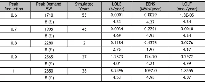
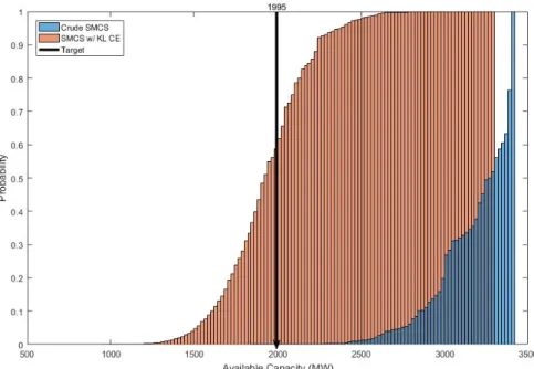
3.4. Sequential MCS with Kullback-Leibler Cross-Entropy ... 36
... 43
Sequential Monte Carlo with Cauchy-Schwarz Cross-Entropy ... 43
4.1. Cauchy-Schwarz Divergence ... 43
4.2. Metaheuristics ... 45
4.2.1. Evolutionary Particle Swarm Optimization ... 45
4.2.2. Particle Movement Equation ... 45
4.2.3. The mutation scheme ... 47
4.2.4. Cauchy-Schwarz CE EPSO parameter tests ... 47
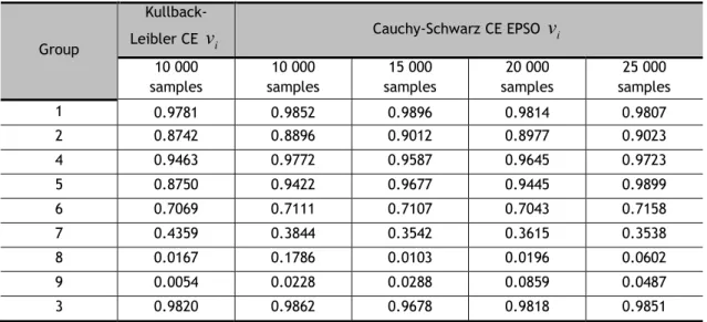
4.2.5. Cauchy-Schwarz CE EPSO results ... 49
4.3. Cauchy-Schwarz Cross-Entropy ... 51
4.3.1. Simple Analytic Example ... 54
4.3.2. Cauchy-Schwarz CE Method Algorithm for Rare Event Simulation ... 55
ix
4.4.2. SMCS with Cauchy-Schwarz CE results ... 61
... 69
Conclusions... 69
5.1. General Conclusions ... 69
REFERENCES ... 73
ANNEX A – CAUCHY-SCHWARZ EPSO CE PARAMETERS TESTS ... 77
ANNEX B – CAUCHY-SCHWARZ EPSO CE TEST RESULTS ... 81
ANNEX C – CAUCHY-SCHWARZ CE PARAMETER TESTS ... 85
xi Figure 2.1 - Models of the development of failure rate throughout time. On the left, typical case of mechanical components subject to wear and tear. To the right typical case of electronic
or electrical components, wherein the aging factors are different. ... 6
Figure 2.2 - Probability Distribution Function of an Exponential Distribution ... 7
Figure 2.3 - Markov diagram for a component with two possible states ... 8
Figure 2.4 - Historical representation of a continuously repairable component ... 9
Figure 2.5 - Graphical representation of the MTTF, MTTR and the MTBF of a component ... 10
Figure 2.6 - Hierarchical Levels [15] ... 11
Figure 2.7 - Generic algorithm for the MCS method ... 15
Figure 2.8 - Values of t distributed according to the Gaussian distribution, following the reverse function of the evenly drawn values of y [11] ... 17
Figure 2.9 - Normal Distribution N (0,1) ... 19
Figure 2.10 - Multi-state Markov chain for modeling the wind speed with transitions between non-adjacent states [14]. ... 21
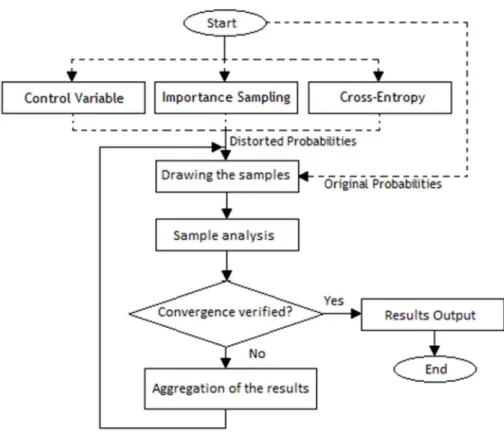
Figure 3.1 – Block Diagram representing the Sequential Monte Carlo method, with the alternative integrated techniques for variance reduction, depicted with dashed lines. ... 32
Figure 3.2 - Single-Line diagram for the test system IEEE-RTS 79 [14] ... 33
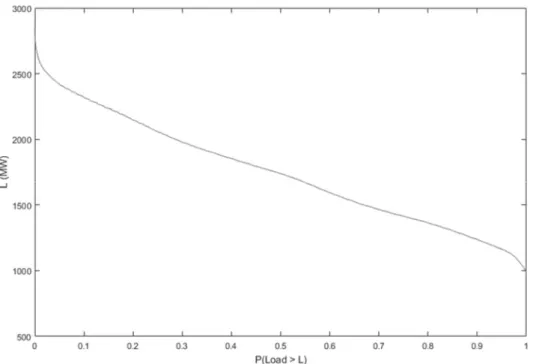
Figure 3.3 – Load cumulative distribution diagram ... 36
Figure 3.4 – Capacity Outage Probability Table (COPT) histogram for 50 000 samples obtained the original FOR and the FOR with Kullback-Leibler distortion for a peak reduction factor of 0.6 ... 38
Figure 3.5 – COPT histogram for 50 000 samples obtained the original FOR and the FOR with Kullback-Leibler distortion for a peak reduction factor of 0.7 ... 39
Figure 3.6 - COPT histogram for 50 000 samples obtained the original FOR and the FOR with Kullback-Leibler distortion for a peak reduction factor of 0.8 ... 39
Figure 3.7 - COPT histogram for 50 000 samples obtained the original FOR and the FOR with Kullback-Leibler distortion for a peak reduction factor of 0.9 ... 40
Figure 3.8 - COPT histogram for 50 000 samples obtained the original FOR and the FOR with Kullback-Leibler distortion for a peak reduction factor of 1.0 ... 40
Figure 4.1 - Illustration of the EPSO movement rule [27]. ... 46
Figure 4.2 - Capacity Outage Probability Table (COPT) histogram for 50 000 samples obtained the original FOR, the FOR with Kullback-Leibler distortion and the FOR with Cauchy-Schwarz EPSO CE distortion for a peak reduction factor of 0.6 ... 51
xii the original FOR, the FOR with Kullback-Leibler distortion and the FOR with Cauchy-Schwarz CE distortion for a peak reduction factor of 0.6 ... 62 Figure 4.5 - COPT histogram for 50 000 samples obtained the original FOR, the FOR with Kullback-Leibler distortion and the FOR with Cauchy-Schwarz CE distortion for a peak reduction factor of 0.7 ... 63 Figure 4.6 - COPT histogram for 50 000 samples obtained the original FOR, the FOR with Kullback-Leibler distortion and the FOR with Cauchy-Schwarz CE distortion for a peak reduction factor of 0.8 ... 65 Figure 4.7 - COPT histogram for 50 000 samples obtained the original FOR, the FOR with Kullback-Leibler distortion and the FOR with Cauchy-Schwarz CE distortion for a peak reduction factor of 0.9 ... 66 Figure 4.8 - COPT histogram for 50 000 samples obtained the original FOR, the FOR with Kullback-Leibler distortion and the FOR with Cauchy-Schwarz CE distortion for a peak reduction factor of 1.0 ... 68 Figure 4.9 – Failure states with contribution to the reliability indices [30] ... 68
xiv Table 3.1 – IEEE-RTS 79 generating system [14]... 34 Table 3.2 – Crude Sequential MCS (SMCS) Generating System Reliability Indices Results for IEEE-RTS 79 [14] ... 34 Table 3.3 – Crude SMCS results for IEEE-RTS 79 with different peak reduction factors. ... 35 Table 3.4 - SMCS with CE results for IEEE-RTS 79 with different peak reduction factors. ... 37 Table 3.5 - Distorted availability introduced by the cross-entropy for different peak reduction factors ... 37 Table 3.6 – Number of load shedding occurrences for different peak reduction values and different number of samples for the original unavailability values ... 41 Table 3.7 - Number of load shedding occurrences for different peak reduction values and different number of samples for the unavailability values with the distortion introduced by the CE method ... 41 Table 4.1 - EPSO test results for Cauchy-Schwarz fitness function with different numbers of samples ... 48 Table 4.2 - EPSO test results for Cauchy-Schwarz fitness function with different population sizes ... 48 Table 4.3 - EPSO test results for Cauchy-Schwarz fitness function for values of max generation ... 49 Table 4.4 - Cauchy-Schwarz CE EPSO results for peak reduction factor 0.6 ... 49 Table 4.5 - Mean years simulated in SMCS to achieve convergence, for the KL and CS distortions ... 50 Table 4.6 – Table for out of service capacities for a small generating system described above ... 54 Table 4.7 – Distortion obtained with the Kullback-Leibler CE and the Cauchy-Schwarz CE .... 54 Table 4.8 – Cauchy-Schwarz CE tests for 10 000 samples with lower bound lb = 0.01 and upper bound ub = 0.99 ... 59 Table 4.9 – Cauchy-Schwarz CE tests for 25 000 samples with lower bound lb = 0.01 and upper bound ub = 0.99 ... 59 Table 4.10 – Cauchy-Schwarz CE tests for 50 000 samples with lower bound lb = 0.01 and upper bound ub = 0.99 ... 60 Table 4.11 – Cauchy-Schwarz CE tests for 50 000 samples with lower bound lb = 0.01 and upper bound ub =
v
t1 ... 60xv Table 4.15 - Mean years simulated in SMCS to achieve convergence, for the KL and CS distortions for a peak reduction factor of 0.7 ... 63 Table 4.16 - Cauchy-Schwarz CE EPSO results for peak reduction factor 0.8 ... 64 Table 4.17 - Mean years simulated in SMCS to achieve convergence, for the KL and CS distortions for a peak reduction factor of 0.8 ... 64 Table 4.18 - Cauchy-Schwarz CE EPSO results for peak reduction factor 0.9 ... 65 Table 4.19 - Mean years simulated in SMCS to achieve convergence, for the KL and CS distortions for a peak reduction factor of 0.9 ... 66 Table 4.20 - Cauchy-Schwarz CE EPSO results for peak reduction factor 1.0 ... 67 Table 4.21 - Mean years simulated in SMCS to achieve convergence, for the KL and CS distortions for a peak reduction factor of 1.0 ... 67
xvii COPT Capacity Outage Probability Table
CE Cross-Entropy
CDF Cumulative Distribution Function CMC Conditional Monte Carlo
CV Control Variables
CS Cauchy-Schwarz
EENS Expected Energy Not Supplied
EPSO Evolutionary Particle Swarm Optimization
EU European Union
HL1 Hierarchical Level One HL2 Hierarchical Level Two HL3 Hierarchical Level Three IS Importance Sampling KL Kullback-Leibler LOLC Loss of Load Cost LOLD Loss of Load Duration LOLE Loss of Load Expectation LOLF Loss of Load Frequency LOLP Loss of Load Probability MCS Monte Carlo Simulation MTTF Mean Time to Failure MTTR Mean Time to Repair PDF Probability Density Function PRF Peak Reduction Factor
SMCS Sequential Monte Carlo Simulation
WF Wind Farm
WTG Wind Turbine Generator
xviii
Failure Rate
Repair Rate R Reliability Q Unreliabilitym Mean Time to Failure r Mean Time to Repair
L Load
Eˆ
Estimated Expected ValueE
Expected ValueVˆ
Estimated VarianceV
Variance
Coefficient of VariationN
Sample Dimension
Standard DeviationC
Covariance
Correlation Coefficient KLD
Kullback-Leibler Divergence KLD
Cauchy-Schwarz Divergence iu
Unavailability of i group for the original distributioni
Introduction
This chapter serves as exhibition of the complex problem at hand, along with its context and the ideas behind this dissertation. Firstly, the context and the importance of problem will be explained as well as the importance of the reliability assessment, followed by the current means of calculating these indices and their significance, finally the motivation for this dissertation will be defended along with its organization.
1.1. Context and Importance of Electric Power Systems Reliability
Assessment
The concept of reliability took a vital Role mid-20th century, when the dimension and complexity of power systems started to rapidly grow. Its modern definition as we know it dates back to 1940 when the U.S. Military started to develop advanced systems of armament which in turn resulted in some of the first reliability studies through computer simulation [1].
Modern power system, nowadays, consist of a complex network of electrical components progressively more interconnected, geographically dispersed across the world, focused on the production, transfer and distribution of electric power, delivering energy downstream to the final consumers. The high number of components, coupled with the demand uncertainties and the fluctuation of energy resources, both renewable and fossil-fueled make the design and its compartmentalized operation extremely complex. Requiring a frequent and precise monitoring by the different operators that compose the system, due to the enormous quantity of components, combined with their unique operation characteristics, there is a possibility of failure of the entire system simply by failing a crucial or a set of crucial components. These phenomena are classified as rare events due to the low probability associated with them.
With its constant growing expansion and complexity, many depend on its normal operation to be as smooth as possible, the economy of a country depends on it, seeing as most of its industry depend on it to boost their activity, as well as possibly its security, with all the electronic equipment used by the military depending mostly to direct connections to the grid, making the power grid of a country a strategic aspect of its defense, presently, not only is the power system delegated to supply the end costumers with energy but likewise to assure that the system functions with a set of standards
in continuity, quality and security, to further develop the economic and social sectors of a modern society [2].
Constant interruptions on electric energy supply can dramatically affect multiple sectors of the economy, forcing them to “buy” reliability, usually in the form of emergency generators, in worst scenarios, these economic agents are forced to move its activities to other countries with high losses in the economic sector as well as a shift of scenery in the social environment.
These setbacks can often be repaired, following short term government measures put in place to attract the industries with other benefits such as tax reductions, financial compensations, etc. Nevertheless, these setbacks lead to more investment both in the power grid and the financial incentives, in turn leading to an unsustainable economic development.
In order to decrease the probability as well as the frequency and the duration of these rare events, more investment is required, however, the tendency to postpone these investments, operating the system near its limits, leaves the decision makers these contradictory requirements when the time comes to reinforce the electric system in order to increase its reliability.
The recent changes in the sector, such as the progressive deregulation with the purpose of creating an electric market, raised the degree of importance to the continuity of service, being the responsibility of the electricity provider to assure a continuous power supply. The operation scenery of the electric power systems has changed, due to new concepts, distributed generation, micro-grids, the increased penetration of energy from fluctuating sources, brought the necessity describe the energy system minutely, to correctly assess its reliability.
1.2. Current Methodology and Motivation
The development of accurate models for the increasing uncertainties and the fluctuating power sources presents itself as a problem with the reliability assessment of modern power systems. Other difficulties are related to the increasing size of the set of the stochastic variables of these models. Even with the current computational power available, the reliability assessment of complex power systems is still time-consuming [3-6].
The creation of efficient methodologies that cope with the new and increasing complexities affecting the reliability of modern power systems is of the utmost importance. The new methodologies must provide satisfactory results with sufficient accuracy, attainable in useful time and must be competitive with existing methods.
The Monte Carlo Simulation (MCS) is, of the available current methods, the most used for reliability assessment of power systems [7-8]. The MCS method is based on the frequentist theory of sampling, which defines the probability of an event as its long-run expected frequency of occurrence [9]. According to this theory, the population mean, in this case is a reliability index, can be estimated by drawing successive samples from the population. The resulting estimate is used to create a
confidence interval for the population mean, which is centered at the sample mean. The MCS methods used for the reliability assessment of power systems are in fact stochastic simulation methods given the random behavior of these systems varying with time [2].
The MCS methods can be subdivided into two different approaches: the non-sequential (non-Chronological) and the sequential ((non-Chronological) [10], the non-sequential MCS method, which is closely related to random sampling, differs from the sequential MCS method which can accurately reproduce the whole cycle of interruptions, as so, this method can easily include all chronological characteristics of power systems into the simulation, such as time fluctuating load models and power sources, the time-dependency of primary energy resources, loss of load cost, maintenance schedules, weather effects, calendar patterns, etc.
1.3.
Hypothesis and Purpose of this Dissertation
For the reasons above, the sequential MCS method can be considered the most complete approach to model accurately the increasing complexity of modern power systems. Unfortunately, the advantages of the sequential MCS method are met by the considerable disadvantageous simulation time necessary to accurately estimate the reliability indices.
The MCS method already has adequate mechanisms to accelerate its convergence time, namely, the Control Variable (CV), or the Importance Sampling (IS), [11]. The Control Variable method assumes it’s possible to calculate an approximate value for that we wish to know, through an analytical method independent in relation to the Monte Carlo. Importance Sampling is based on a distribution distortion in order to increase the probability of rare events. This technique seeks to reduce the variance without changing the expected value.
The purpose of this dissertation is to research more ways to accelerate the MCS method. The research explores the notions of importance sampling and Cauchy-Schwarz Probability Distribution Function (PDF) distance, and further developing the implementation of cross-entropy methods currently based on the Kullback-Leibler PDF distance. This study is motivated by the theoretical hypothesis that the optimal distribution distortion would require only one iteration of the method to converge, and therefore obtain accurate results with less simulation time. That being said we, will be looking for a parallelism between the current methodologies to facilitate the implementation of new algorithms to distort such distribution.
1.4.
Dissertation’s Structure
This dissertation’s work is compartmentalized in 5 chapters, that obey the following structure: Chapter 1 consists of a brief, yet important, contextualization of the problem, this dissertation and its studies will revolve around, along with some of the implications of power systems reliability in the world as we know it and lastly, the motivation and scope of this work.
Chapter 2 serves as a more detailed and structured introduction to the current methodologies. Starts with a brief explanation on reliability assessment, followed by the different reliability indices, describing the hierarchical levels, the analytical methods, finishes with the MCS and the basic concepts associated, as well as the complementary mechanisms used in conjunction with the MCS to accelerate its convergence.
Chapter 3 will introduce the model IEEE RTS 79 used in all of this work’s tests, as well as, show the current CE and MCS results and efficiency, through a battery of different tests using both methods in conjunction and the crude MCS alone. Finishes by comparing and discussing the obtained results.
Chapter 4 introduces the Cauchy-Schwarz Inequality, along with the possibilities of introduction in the MCS method, investigates the parallelism with the current Cross-Entropy methods based on the Kullback-Leibler Divergence. The second part of this chapter presents the results obtained with the new method and compares them with the current one.
Chapter 5 finally closes this dissertation with the conclusions attained in the previous chapters, trough research and extrapolations, and the reference list to the main scientific knowledge contributors.
State of the Art
2.1. Reliability Assessment
Reliability is a branch of engineering knowledge that seeks to establish behavior models for systems with components subjected to, partial or full, malfunctions that may impede the normal operation, for which the system was conceived [11].
The reliability assessment studies concern systems, more or less complex. The representation of such failures in the system’s equipment is done with basis in probabilistic models, allowing us to represent the uncertainty of those events, especially when there is insufficient statistical sampling [11].
Due to the probabilistic nature of the events, it’s assumed that such events related with the system occur randomly, and there is no way to predict with enough precision the moments when the components fail. Therefore, probabilistic distributions are used, based on the statistical analysis of the behavior of similar systems of components [11].
As an example, if we assume X as random variable representing a component’s lifetime the likelihood of such component surviving a certain time t or past that certain time t, can be respectively represented as and . The probability of a component surviving past a certain time, is designated as reliability, which can be represented by the letter R. We can establish:
t
P
X
t
R
, (2. 1)if we assume f(x) as the PDF of X, we have
tf
x
dx
t
R
. (2. 2)Another important concept associated to these studies is the failure rate, often represent by the Greek letter λ, the failure rate is defined as follows:
t
R
f
t
t
t
R
dR
t
t
dt
. (2. 3)The failure rate can be perceived as the frequency with which an engineered system or component fails, in a determined interval between t and t+dt. Upon expansion of the following equation
t
dt
dR
R
t
t
, (2. 4) we obtain
dR
t
t
R
dt
t
t Rt
0
11
, (2. 5) which is equivalent to
e
t tdtt
R
0 . (2. 6)Thus we have the reliability of a component as function of the failure rate. If the failure rate is considered constant throughout time, λ λ, and so independent from time, comes
t
e
tR
(2. 7)As equation 2.7 shows, this is one of the justifications for the use of exponential distribution. Nevertheless, the failure rate can’t always be assumed as constant, and so it’s possible to observe two different patterns for its evolution throughout time in the following figure.
Figure 2.1 - Models of the development of failure rate throughout time. On the left, typical case of mechanical components subject to wear and tear. To the right typical case of electronic or electrical components, wherein the aging factors are different.
2.1.1. Exponential Distribution
If a random continuous variable, is non negative, X will present an exponential distribution with the failure rate λ, if its PDF it’s given by
t
e
tf
, for t≥0, (2. 8)if we integrate function f(t), we have 1, which in turn represents a PDF:
Figure 2.2 - Probability Distribution Function of an Exponential Distribution
Therefore, we can define the PDF of an Exponential distribution as:
0
,
0
0
,
)
;
(
x
x
e
t
f
t . (2. 9)The exponential distribution plays a practical central role in the establishment of component behavior models, particularly in power systems, despite other distributions being used in reliability models. Namely the Gauss distribution and Weibull, having no memory, is a good representation of electrical and electronic systems, in particular the ones subjected to maintenance in order to keep them working within their lifetime.
2.1.2. Markov Models for repairable components
The Markov models assume a special importance, because they can serve as a reference model to most of the studies. However, they require a certain data precision, which in many cases it’s not compatible with the existing or the stored database. Nonetheless the Markov processes allow us to model many phenomena, in this particular case the electric power systems [11-13].
In order to build a Markov model for the reliability assessment problem, it’s necessary that we begin with defining the possible residing states for a component. In this case, it can be as simple as a component being in two states, enabled (E) and disabled (D). It’s also necessary to describe the transitions between states: admitting such state might change or maintain we have the following possible Markov diagram:
Figure 2.3 - Markov diagram for a component with two possible states
Assuming that time is a sequence of discrete leaps, we are in the presence of a discrete Markov process, and the system’s evolution is a sequence of states. This allows us to mathematically represent the process through the so called Markov matrix, that states
1
1
1
1
t
P
t
P
t
P
t
P
D E D E
, (2. 10) with:
P
E
t
- Probability of the component being enabled in the time instance t;
P
D
t
- Probability of the component being disabled in the time instance t; λ – failure rate (constant); µ - repair rate (constant);
2.1.3. Basic Indices in Electrical Systems Reliability
In most of the electrical reliability assessment studies, the analysis and calculus are based in basic statistical indices, such indices, commonly represented by traditional letter are as follows [11]:
λ – Failure Rate, [failures/year]; FOR – forced outage rate, [%]; µ – Repair Rate, [year-1];
r – Mean time to repair, [hours]; U – unavailability, [hours/year]; PNS – Average power cut, [kW, MW];
E – Average Annual Non Supplied Energy, [kW, MW/year]
The first five are a result of the probabilistic models, the last two measure the impacts in the system, the average power cut corresponds to the expected value of the power cut distributions because of the unscheduled service interruption
The average annual non supplied energy corresponds to the expected value of the product of each power cut in each incident by the respective duration.
Although there are more indices that help define a systems reliability, but these five form the necessary conceptual basis.
2.1.4. Mean time to failure and to repair
The operation of a component continuously repairable, may be represented as follows:
Figure 2.4 - Historical representation of a continuously repairable component
The definition of the mean time to failure and mean time to repair is depicted by the following equations [11] [13]:
1
1
f n i fin
t
MTTF
m
f , (2. 11)
1
1
r n i rin
t
MTTR
r
r . (2. 12)These indices can be easily diagrammed, as it can be seen below, along with another important index, the mean time between failures (MTBF),
MTBF
m
r
:Figure 2.5 - Graphical representation of the MTTF, MTTR and the MTBF of a component
Therefore, the probabilities of a component being available or not, at any moment are given by:
r
m
r
Available
P
(
)
’ (2. 13)
r
m
m
le
notAvailab
P
(
)
. (2. 14)2.2. Reliability Indices
Reliability assessment studies, as we would expect result in reliability indices that help define the systems and characterize the service quality. Reliability indices can provide information on the reliability of a system, which are most commonly associated to the planning phase. These indices can be called predictive indices, in turn there are the past performance indices which refer the actual system reliability, presenting the events observed in the studies. Considering this dissertation addresses mostly the planning phases with simulation methods, only predictive indices are used [14].
The main objective of these studies is not to solve decision problems, but instead to provide quantitative information, whether of economic nature or risk, which constitutes aid elements to decision. Below are some of the most common reliability indices, addressing frequency, duration, cost and even the energy associated with each event [13]:
Load of Loss Probability - LOLP [%]– Probability associated with load shedding;
Load of Loss Expectation - LOLE [hour/year} - Average hours with load shedding during a year;
Expected Energy Not Supplied – EENS [MWh/year] – Average energy shedding during a year;
Expected Power Not Supplied – EPNS [MW] – Average load shedding;
Loss of Load Frequency – LOLF [occurrence/year] – Average number of load shedding occurrences during a year;
Loss of Load Duration – LOLD [hour/occurrence] – Average duration of load shedding occurrences;
Loss of Load Cost – LOLC [currency/year] – Average cost of load shedding during a year;
Although there are more indices that help define a systems reliability, these are the ones that will be use in this dissertation due to the nature of this work.
2.2.1. Hierarchical Levels of Reliability of a Power System
Power systems can be divided in three hierarchical levels (HL). Firstly, the HL1 refers to the generation facilities, HL2 is concerned to the so called composite system, which includes both the generation and transmission facilities, lastly HL3 concerns the entirety of the power system, including the composite systems and the distribution facilities up to consumer load [15].
In this dissertation we will mostly deal with HL1 reliability, which is enough to test the efficiency of current and the researched methodologies.
2.2.2. Hierarchical Level 1 (Generating System)
Planning the expansion or the operation of a production system, requires taking into account the economic rationalization objectives and goals or restrictions associated with service quality assurance. In particular, it’s imperative, as a first concern, to focus in having sufficient production capacity to supply the load (forecast) system [11].
The necessity for these studies results from the dramatic consequence, of not having enough capacity to satisfy the peak demand, that in turn derives from component breakdowns, unseasonable forced outages and schedule maintenance. Therefore, the determination of the appropriate values of availability of power production, in the form of installed capacity in the core, is at the center of static reserve studies. In general, these studies attempt to determine the suitability of building up a central or adding new groups, so that we may numerically determine the assurance that the system load will be powered entirely.
2.2.3. Hierarchical Level 2 (Composite System)
These HL2 studies, no longer concern only the generating systems as well as the transmission, as so, it’s required to include the detailed model for the transmission grid. Another important aspect is the inclusion of more restrictions in comparison to the HL1 studies, due to the characteristic of components that compose the transmission grid, such as, voltage and loading limits of the circuit and the active and reactive power transit [2] [15]
The more complete model approach of these studies, allows, in turn, for a more accurate, way of determining the effects of the geographic dispersion of the loads and energy sources. The necessity for these studies comes from the independent nature of the components, that can cause load shedding even with the generating system fully operational, as such, they attempt to determine the suitability of building new transmission lines or reinforcing existing ones, so that we may numerically determine the assurance that the composite system.
2.3. Analytical Methodology
Analytical methods, aim to solve the mathematically modeled problem, resorting to the calculus of the reliability indices through the obtainment of the probability mass functions. This approach is computationally more efficient, however, the systems have to be simple to mathematically model and with a reduced number of components due to exponential increase in complexity [14] [11].
2.3.1. Capacity Outage Probability Table
The capacity outage probability table, is one of the steps to calculate a basic system’s reliability indices, this table is an enumeration of all possible systems states and their probability of occurrence. Nevertheless, the information obtained calculating it, is of the utmost importance because it gathers pertinent values and allows us to proceed to the calculus of the Loss of Load Probability and other reliability indices [11].
2.3.2. Loss of Load risk calculus
Given the values obtained from the capacity outage probability table, it’s possible to calculate the risk values known as LOLP and LOLE, both concern to the probability of load shedding events throughout an evaluation period commonly set as a year. The main difference between LOLP and the LOLE, is that the LOLP is dimensionless, considered as a probability percentage and the LOLE expresses the same value in days or hours per year [11]. With that in consideration the formula is as it follows:
n ip
x
ip
L
X
X
iLOLP
1 max . (2. 15) In which:
p
x
i - lost capacity probability ofx
i kW or MW:
X
max - total installed capacity in Kw or MW;
L
- load peak;
p
L
X
max
X
i
- probability that the load peak exceeds the availablecapacity at the i state; n – total number of states;
365
)
(
Risk
LOLP
2.4. Simulation Methodology
Simulation methods are mostly based in the MCS [3] [8], these methods integrate optimization techniques into simulation analysis, due to the complex nature of some of the simulations the objective function may prove hard to evaluate and optimize.
The MCS is a powerful tool, evaluating phenomena which can be characterized as probabilistic. The main idea behind the model is to form a representative sample of the system’s behavior, by drawing and analyzing each state in order to evaluate the average values of the results and other parameters, and thus, deducing the system’s behavior from the behavior of the sample.
The estimates that result from these studies, do so, not only delivering the reliability indices, as well as a confidence interval, plausible to obtain due to the computer-based simulation of the stochastic behavior of these mathematically modeled systems [12-13].
The main advantages that derive from using the MCS are:
It allows us to use any probability distribution function; Easy to include dependency relations between events; Easily adjustable to any system alterations;
Despite the obvious advantages, this method can present as well some disadvantages:
Great number of experiments, necessary to perform;
If the study of each state proves to be complex, it may end up requiring a great computational effort, and in turn more computational time;
The MCS method, as previously said, can be divided in two approaches, classified according to how each system state is sampled. If the state’s space representation is used then, we might call the MCS as non-sequential or non-chronological, in turn, if the state’s sampling, is done following a chronology of the events such as those in figure (2.4), the method is called sequential or chronological. A more simplistic and metaphoric approach would be comparing the non-sequential MCS states to pictures, a collection of static images of the system in different moments, and the sequential MCS states chronology, as a film’s timeline, in both methods each state is the aggregation of the states of each component [12-13].
The sequential MCS allows as well to integrate generating capacity from fluctuating or time dependent power sources such as renewable resources, which are modeled with uncertainty.
Drawing the samples (states) to analyze;
Analysis of the sample depending on the value to study;
Preforming a convergence test to verify if the estimate possesses the required accuracy and quality;
Figure 2.7 - Generic algorithm for the MCS method
2.4.1. Non-sequential MCS method initialization
As previously stated the non-sequential MCS, draws each sample, as static images of the system’s stochastic behavior, that being said, each components current state is completely independent from previous or future states [14].
The estimated reliability indices are mathematically calculated as
N iH
x
iN
X
H
E
11
ˆ
, (2. 17)considering , , , … , to be a real vector, in which x1, x2, x3, …, xn,are the sampled system
states, with N concerning the number of samples, and H being the test function every state is submitted, H(xi) will be the outcome in the following terms
Xs i Xf i iif
if
x
x
S
S
x
H
0
1
, (2. 18)where,
S
XfandS
Xsare respectively all the failure states and the success states.2.4.2. Sequential MCS method initialization
The sequential approach, requires more information, it’s no longer sufficient knowing the component’s FOR, it’s now necessary to know the PDF functions associated with the time to failure and time to repair. If we assume exponential distributions these will be characterized by the failure and repair rate [11].
It’s also necessary to have a model for the load fluctuation based on a forecast, it can consist of a deterministic load curve, with no uncertainty, that must be chronological, in other words it can no longer be an accumulated load diagram, otherwise it might as well be a load forecast with a probabilistic model or uncertainty.
The generation of a random time value t normally distributed (Gaussian function), is done, firstly by evenly drawing a value y in [0,1], and then intersecting from the Y-axis the distribution curve, we find the correspondent value of t, due to the exponential character of the function,
t
e
y
F
1
t
, (2. 19)it’s possible to resort the inverse function,
y
F
t
1y
1
log
1
. (2. 20)As so this allows us to evenly distribute in [0,1] and immediately calculate the exponential distributed value of y.
Figure 2.8 - Values of t distributed according to the Gaussian distribution, following the reverse function of the evenly drawn values of y [11]
Consequently, all the simulated lifecycles are aggregated to create the system lifetime, which in turn will be evaluated every step of the way to see if the systems composition is enough to supply the respective load in that moment, to guarantee each component resides in 2 states (on and off). The timeline simulation is done by chaining successively drawn times to failure and times to repair [14]. The estimated reliability indices are mathematically calculated as
N i S n n ix
H
N
X
H
E
1 11
ˆ
, (2. 21)considering , , , … , , ∈ ℕ, is the chronologically sampled system states x, concerning the period i, with N the number of periods simulated, and H being the test function every state is submitted, the outcome will be in the following terms
n S n n S n nT
d
H
H
x
i1
ix
x
1 1
. (2. 22)where is the nth state of the sequence, T is the total duration of the simulated period (typically T
= 8760 h), d ( ) is the duration of the state and H ( ) is the outcome of (2.18) with as argument.
2.4.3. MCS method convergence
In the MCS, we estimate E
H , from equations (2. 16) and (2. 20), depending on the simulationapproach, however Eˆ
H , is an estimate and not the “real” expected value E
H , which is unknown.As in most sampling processes, the average sample value, distributes itself around the “real” value in such way that the uncertainty of the estimate may be represented as a variance V ˆ
E
H of theestimator [11]:
N
H
V
H
E
V
ˆ
, (2. 23)where V
H is the real variance of H, as this one is also unknown, we resort to an unbiased estimator, given by,
N iH
x
iE
H
N
H
V
1 2ˆ
1
1
ˆ
. (2. 24)As shown in the equation above (2. 23), we can interpret the uncertainty in the Eˆ
H estimate,reversely proportional to the sample dimension N. In order to limit this uncertainty, we can establish a convergence criterion to stop the MCS, through the definition of a relative uncertainty, based in the variation coefficient designated as β, such that
2 2ˆ
ˆ
H
E
H
E
V
, (2. 25)rearranging the equation, to putting N in evidence, and substituting V ˆ
E
H , we arrive to the followingexpression
ˆ H
2E
H
V
N
. (2. 26)Through the above expression we can finally arrive to the conclusion that, for a given precision of the estimate’s β, to decrease the number of drawings N, or the size of the sample, we must first reduce V
H .This forms the conceptual basis of the variance reduction schemes which aim to reduce the computational effort involved in the calculation of an estimator, for a given predefined accuracy β.
2.4.4. Confidence interval
Knowing the variance V
E
H
, allows us to easily estimate a confidence interval (CI) for Eˆ
H ,and that means, there is a given probability the calculated interval contains the exact value we are looking for. Based in the central limit theorem [16], that states the sum of independent identically distributed variables
N iH
iN
Z
1x
, (2. 27)tends towards the normal (Gaussian) distribution N (0,1) with average µ=0 and a variance σ2=1, as it
can be seen in figure (2.9), with a symmetric interval centered in 0 and with a half-width of two standard deviations, corresponding to a probability possible of calculating through the integral of the respective PDF:
Figure 2.9 - Normal Distribution N (0,1)
For any real positive value Z, it’s possible to find the opposing values (+z) and (-z), between which Z lies with a certain probability 1-α,
z
Z
z
1
the number z can be obtained via the cumulative probability distribution as,
1
2
Φ
1
2
)
(
Φ
z
P
Z
z
z
1
, (2. 29)therefore, determining a confidence interval CI for Eˆ
H , in a MCS method, originates:
N
H
E
N
H
E
CI
1
ˆ
Φ
11
2
ˆ
,
ˆ
Φ
11
2
ˆ
. (2. 30) For example, defining a variation coefficient β=0,05 or 5%, and CI=95%, the confidence interval is:
N
H
E
N
H
E
CI
95
%
ˆ
,1
96
ˆ
,
ˆ
,1
96
ˆ
. (2. 31)2.5. Modeling Generating System Components
2.5.1. Conventional Generating Units
Conventional generating units are still the more common source of energy, mostly composed of thermal energy conversion units, commonly based of fossil-fuel, such as petroleum, natural gas and charcoal, but also derived from nuclear sources conversion through thermodynamic cycle [14].
These unit’s failure/repair state cycles can be easily represented by the Markov model for a two state component, with the enabled state representing the fully functional operating unit with maximum capacity, and the disabled sate as the opposite. However, there may be some cases in which a component might not be in any of those two states, but instead in a “partial damaged” state, in which the unit is operating at a percentage of its total capacity and therefore not fully operational neither disabled.
2.5.2. Hydro Generating Units
Hydro generating units nowadays occupy a considerable percentage of the any country’s generating system. These units convert the potential energy of the water to electric energy, through controlling the volume of water and the fall distance that interact with the dam’s generators, as such, they can also be modeled the same way as the conventional generating units,
However, the capacity time-dependent model for these units, is complex, due to the ties with the reservoir storage, weather, and the inflows. One simple yet crude approach, is to resort to hydrological series, historical recordings, in order to forecast the production each month. Doing this by capturing the proportional relation between the reservoir availability and the energy produced [17-18]. Therefore, modeling these units’ in the sequential MCS can be easily done with the hydrological series, due to the chronological nature of the method.
2.5.3. Wind Farms
Wind farms consisting of an aggregation of multiple independent wind turbine generators, convert the kinetic energy of the wind to electricity. Assuming all the wind generators to be equal within a farm, allows us to model such power source using the multi-state Markov model, as pictured below, with each transition following an exponential distribution [14],
Figure 2.10 - Multi-state Markov chain for modeling the wind speed with transitions between non-adjacent states [14].
As with the hydro generating units, these units follow a capacity time-dependent model, with the aid of the historical records for hourly wind series, which capture the hourly production in a percentage of the total capacity. It’s possible to integrate them in the MCS method without any trouble, mainly, due to the needlessness to build spatial and time correlation models, since these correlations are included in the historical recordings, and naturally integrated in the simulation timeline.
2.5.4. Transmission Lines and Transformers
Assuming the operating limits are constant these components are also modeled by the Marko model for two state component with transitions that follow an exponential distribution [14].
2.5.5. Load
Loads are often modeled using a chronological representation with fluctuating load levels for every hour of the year, forecast uncertainties can also be introduced in the model through normal distribution [16], with a probability for each forecast scenario.
The chronological nature of the load, also allows for an easy integration with the sequential MCS, which follows the load level throughout the simulation period matching them with the respective available capacity to determine if the load shedding occurs, adding to this, each load bus has its own hourly load profile in percentage of its peak load, obtained by dividing the peak load of that hour by the peak load of the year.
2.6. Simulation Algorithm
The algorithm for the sequential MCS method for the HL1 reliability assessment follows the next few steps [14]:
1. Defining the initial parameters, maximum simulation period, NMAX, the relative uncertainty
β, initialize the counters time, h=0, and NYEAR =1;
2. Update the simulation time: h: = h + 1;
3. Select a system state (select the availability of the components according to their stochastic failure/repair cycle model and the capacity time-dependent model, select the load level, etc.)
4. Evaluate the system state selected (compose the state and check if the load level can be supplied with the available generating and/or transmission capacity without violating
operating limits; If not, apply remedial actions, such as generation re-dispatch and/or load shedding)
5. Update the outcome of the test functions of the reliability and other indices
6. If h = 8760, store the reliability indices, update their relative uncertainty (β), and advance, if not, go back to step 2
7. If NYEAR is equal to NMAX or if the relative uncertainties of the reliability indices are less than
the specified tolerance, stop the simulation; otherwise, NYEAR = NYEAR + 1, h = 0, and go back
to step 2
2.7. Convergence Accelerators
As seen before, it’s possible to decrease the computational effort and the number of samples, maintaining the same precision β, and the expected value Eˆ
H , only by diminishing the variance
HV . The following paragraphs describe two effective techniques to accelerate the MCS convergence [11].
2.7.1. Control Variable
This method assumes it’s possible to calculate a value approximate to the real one which we wish determine, through an analytical method independent from the MCS. For instance, if we wish to determine the LOLP of a composite system, we can perceive that LOLPg, calculated considering only
the generating system, may be an approximation to the correct value of the compound system and even some well-correlated manner with him [11] [14].
The MCS will only be used to calculate the difference between both values. In order to insure that the convergence is effective, it’s imperative, considering we wish to achieve a quick convergence speed, choosing a highly correlated value with the solution of the problem, a correct control variable, therefore.
Considering Z as a random variable with the result deriving from the approximate analytic model, and that is strongly correlated with H (LOLP), we may define this new auxiliary random variable Y as,
Z
E
Z
r
H
Y
, (2. 32)where r is a real parameter, as said before it’s easy to prove that Y and H have the same expected value, and the variance is as follows:
Y
E
H
r
E
Z
E
E
Z
E
H
E
, (2. 33)
Y
V
H
rE
Z
V
, (2. 34) withrE
Z
as a scalar,
Y
V
H
rC
H
Z
r
V
Z
V
2
,
2 , (2. 35)
H
Z
C ,
is the covariance between H and Z, the theoretical value of r that minimizesV
Y
may be obtained with the derivative of the right member of equation (2.34) equating to zero,
2
,
0
2
rV
Z
C
H
Z
. (2. 36) Substituting
Z
V
H
Z
C
r
,
in the expression above we have,
Y
V
H
C
V
H
Z
Z
V
2,
, (2. 37)now
C
2
H
,
Z
is, by definition, equal to
2V
H
V
Z
, in which ρ is the correlation coefficient between H and Z, then
Y
V
H
V
1
2
. (2. 38)If Z and Y are correlated,
V
Y
will be less thanV
H
, as Y and H have the same expected value,E
H
may be estimated in a more efficient manner by sampling Y than F,
* 1 *1
ˆ
N iY
iN
H
E
, (2. 39)in which N* is the new number of system state drawings, necessary and smaller than N, the reason between N/N* is the acceleration measure introduced by the control variable
2 *
1
1
N
N
. (2. 40)This result shows that the more correlated are the variable that is intended to estimate and the analytical value calculated, the greater the acceleration introduced by the method.
2.7.2. Importance Sampling
This technique is based in the distortion of the probability distribution of xi, in turn distorting H(xi)
and increasing the probability of occurrence of rare events, such as Loss of Load. Like the control variable this method aims to reduce the variance without perturbing the expected value.
Recalling that the probabilistic analysis of a power systems can be seen as determining the expected value of the analysis function of the system states, such that [11] [14],
i N iH
x
if
x
N
H
E
11
, (2. 41)where
f
x
i is the probability distribution function, if we considerg
x
i the distorted PDF, calculated through the next expression,
x
if
x
ik
f
x
i
g
1
, (2. 42)K represents the acceleration coefficient, and directly affects the method’s efficiency, therefore is required to choose an adequate value. Now, multiplying and dividing the interior of the summation in equation (2. 40) by
p'
x
i we can rewrite it as:
i i i N i ig
x
g
x
x
f
x
H
N
H
E
11
. (2. 43)Now the system state’s sampling will follow the probabilistic distribution of
g
x
i , as previouslymentioned this too doesn’t affect the expected value however it can considerably reduce the variance,
N i i i ig
f
x
x
E
H
x
H
N
H
V
1 21
1
. (2. 44)Theoretically speaking, there is a value of
g
X
, that could render the variance as zero,
f
X
LOLP
H
X
X
g
*
, (2. 45)However, such value would require of us to know the exact value
LOLP
E
H
which we wish to estimate, creating a circular reference in the calculus,E
H
may now be estimated in a more efficient manner by samplingg
x
i thanf
x
i resulting,
i i N i ig
x
x
f
x
H
N
H
E
* 1'
1
ˆ
, (2. 46)in which N* is the new number of system state drawings, necessary and smaller than N, due to the acceleration introduced by the distorted distribution
![Figure 2.8 - Values of t distributed according to the Gaussian distribution, following the reverse function of the evenly drawn values of y [11]](https://thumb-eu.123doks.com/thumbv2/123dok_br/15495086.1043164/39.892.200.689.108.345/figure-values-distributed-according-gaussian-distribution-following-function.webp)
![Figure 2.10 - Multi-state Markov chain for modeling the wind speed with transitions between non-adjacent states [14]](https://thumb-eu.123doks.com/thumbv2/123dok_br/15495086.1043164/43.892.155.724.698.1039/figure-multi-state-markov-modeling-transitions-adjacent-states.webp)
![Figure 3.2 - Single-Line diagram for the test system IEEE-RTS 79 [14]](https://thumb-eu.123doks.com/thumbv2/123dok_br/15495086.1043164/55.892.206.696.98.757/figure-single-line-diagram-test-ieee-rts.webp)