Spatio-temporal Modelling of Tornados with
R-INLA, at the county-level in Texas and
Oklahoma
Spatio-temporal Modelling of Tornados
with R-INLA, at the county-level in
Texas and Oklahoma
by
Angela Afonso Rodrigues
Dissertation supervised by
Jorge Mateu Mahiques, Ph.D
Institute of New Imaging Technologies (INIT),
Universitat Jaume I, Castellón, Spain
Co-supervised by
Fernando Santa, M.Sc.
NOVA Information Management School (NOVA IMS),
Universidade Nova de Lisboa, Lisbon, Portugal
and
Edzer Pebesma, Ph.D
Institute for Geoinformatics,
University of Münster, Münster, Germany
ACKNOWLEDGNEMENTS
I would like to express my uttermost and sincere gratitude my supervisor Prof. Dr.
Jorge Mateu Mahiques, for all his support and guidance throughout the development
of this thesis. It was a great honor to learn from such a great professional, and be
advised by his positive and whole-hearted personality. I also express my gratitude to
Dr. Pebesma and Fernado Santa, for accepting and co-supervising this thesis.
I am also indebted to Prof. Doctor Marco Painho, for his support and follow-up during
the course of the whole program.
In addition, I would like to express my gratitude to Dr. Marta Blangiardo, Dr. Barry
Rowlingson, and Dr. Peter Diggle for their prompt and effective advice.
I dedicate this thesis to my parents, for the comfort, support and spiritual shelter that
only a family can provide. To my brother, for being the greatest human being alive,
and for his limitless support and patience with me.
To my friends Pedro R., Chenah J., Dave M., Vânia O., and Carina D., who always
cared for me with a truthfully and unbiased friendship. For all their support, advice
and great moments shared over this period.
Last but not least, to Abuzar P., for the comfort and care; for the unlimited and
unconditional support; for all the moments and places; for standing by, and holding
on; for “this side of the ocean”.
Spatio-temporal Modelling of Tornados
with R-INLA, at the county-level in
Texas and Ocklahoma
ABSTRACT
The United States of America is the county in the world that is more prone to tornado
occurrence. This fact led many researchers, for the past years, to study and formulate
theories about tornado occurrence, and which factors promote tornadogenesis. The
theories around tornados are always coupled with an attempt to predict their
occurrence, for better disaster alertness, and response, in case they happen. At the
country level, the tornado occurrence is highly studied and understood. But the same
does not happen for the state level, or county level.
In this thesis, it is proposed a statistical model to characterize the occurrence of
tornados in a state, given physical (terrain roughness and land-cover types)and
demographic properties of its counties. This model also takes into consideration the
spatial and temporal dimensions, as well as a space time interaction component. This
model was applied for Oklahoma and Texas.
The model with the covariates fits Texas‟ tornado occurrence, but for Oklahoma, only
the spatio-temporal formulation can be applied.
For Texas, the model explains the covariates as being congruent with the low-level
inflow hypothesis, with tornados decreasing in zones where natural barriers for the
flow can be constituted.
Under the Bayesian framework, maps of spatial risk and probability of tornado
occurrence for Texas and Oklahoma were computed, that can be used to make
predictions in the future.
KEYWORDS
Tornados
County-level tornado modelling
R-INLA
Arcpy
Python
Point-processes
Areal Modelling
Spatio-temporal analysis
Spatio-temporal modelling
Bayesian Statistics
ACRONYMS
LULC – Land-use Land-cover
FS – Fujita Scale
CWA – County Warning Areas
NOAA – National Oceanic Atmospheric Administration
SPC – Storm Prediction Center
USA – United States of America
WAIC – Wanabe-Akaike Information Criteria
INLA – Integrated Nested Laplace Approximation
TPI – Topographic Position Index
RI – Roughness Index
DEM – Digital Elevation Model
Kinhom – Inhomogeneous K-function
BYM – Besag-York-Mollie
PIT - Probability of Integral Transform
CPO - Conditional Predictive Ordinates
MCMC – Markov-Chain Monte Carlo
CrI – Credible Interval
CAR – Conditional autoregressive
RW – Random Walk
STI – Space-Time Interaction
STITI – Space-Time Interaction Type I
SD – Standard Deviation
ST – Space Time
INDEX OF TEXT
ACKNOWLEDGNEMENTS ... iii
ABSTRACT ...iv
KEYWORDS ... v
ACRONYMS ...vi
INDEX OF FIGURES ...ix
INDEX OF TABLES ...xi
1. INTRODUCTION ... 1
1.1 Tornado Dataset: some statistics and remarks ... 2
1.2 The Tornado Alley ... 6
1.3 Why so many tornados? ... 7
1.4 Final Problem Statement ... 10
1.5 Objectives ... 10 1.6 Research Questions ... 11 1.7 Thesis Structure ... 11 2. THEORETICAL FRAMEWORK ... 12 2.1 Bayesian Framework ... 12 2.1.1 Bayesian Statistics ... 12 2.1.2 Bayesian Inference... 12
2.1.3 R-INLA: The Integrated Nested Laplace Approximation ... 13
2.1.4 Spatio-temporal modelling under the Bayesian Framework ... 16
2.2 Modelling Tornado Occurrence ... 18
3 STUDY AREA ... 19
3.1 Texas ... 19
3.2 Oklahoma ... 22
4 RESOURCES USED ... 23
4.1 Data description ... 24
4.1.1 Tornado Occurrence in North-America ... 24
4.1.2 Digital Elevation Model ... 25
4.1.3 Population ... 26
4.1.4 Land Use/ Land Cover ... 28
4.2 Description of Software used ... 29
5 METHODOLOGY ... 30
5.1 Point Processes ... 30
5.1.1 Intensity ... 30
5.1.2 Intensity as a function of covariates... 31
5.1.3 Correlation ... 32
5.1.4 Spatio-temporal Inhomogeneous K-function ... 33
5.2 Lattice Approach ... 34
5.2.1. Why INLA? ... 34
5.2.2. Data manipulation and database construction ... 34
5.2.3. Accessing model quality ... 35
5.2.3.3. Distribution of the random effects ... 36
5.2.4. Modelling Technique and formulation ... 36
5.2.5. About the model outputs ... 39
6. RESULTS AND DISCUSSION... 40
6.1. Point Processes ... 41
6.2. Lattice Approach ... 46
7. CONCLUSIONS AND FUTURE WORK ... 63
8. BIBLIOGRAPHIC REFERENCES ... 65
9. ATTACHMENTS ... 71
A.1. Python script for DEM geoprocessing ... 71
A.3. Python Script to construct the buffer of 40Km outside and give the points of the
polygon ... 75
A.4. Adjacency matrix for the counties ... 76
A.5. Visual representation of the point process pattern by FScale ... 77
A.6. R-Code for Point Processes... 80
A.7. R-code for Lattice approach ... 88
A.8 Packages used in R ... 102
INDEX OF FIGURES
FIGURE 1-1.EVOLUTION OF ABSOLUTE TORNADO YEARLY COUNTS IN USA, DURING THE PERIOD OF 1950-2015;THE LINEAR SMOOTHER DENOTES THE MAIN TENDENCY OVER THE YEARS. DATA SOURCE:SPC2016A. ... 2
FIGURE 1-2.ABSOLUTE YEAR COUNTS OF TORNADOS PER YEAR, PER FUJITA SCALE.THE TREND LINE, COMPUTED BY ´LOESS´
METHOD, SHOWS THE GENERAL TENDENCY FOR THE MENTIONED PERIOD.DATA SOURCE:SPC2016A. ... 4 FIGURE 1-3.ANNUAL TOTALS OF PROPERTY LOSSES,FATALITIES AND INJURIES, SUBSEQUENT OF TORNADOS, DURING THE
PERIOD OF 1950-2015(DATA SOURCE:SPC2016A) ... 6 FIGURE 1-4.STATES THAT COMPOSE THE TORNADO ALLEY ZONE, OR, IN OTHER WORDS, STATES THAT HAVE MAJOR
INCIDENCE OF TORNADO RECORDS IN USA. ... 7 FIGURE 1-5.NUMBER OF ABSOLUTE COUNTS OF TORNADOS PER YEAR, FOR ALL STATES OF THE TORNADO ALLEY.DATA
SOURCE:SPC(2016A) ... 9 FIGURE 3-1.LOCATION OF TEXAS IN USA, WITH REPRESENTATION OF MAIN CITIES, AND SURROUNDING STATES. ... 20 FIGURE 3-2.NUMBER OF TORNADO REPORTS IN TEXAS, OVER THE PERIOD FROM 1970 TO 2015, REPRESENTED BY
FSCALE, WITH TREND LINE COMPUTED BY “LOESS” METHOD.SOURCE SPC2016A. ... 21 FIGURE 3-3.MAP OF TEXAS WITH THE NUMBER OF TORNADOS PER COUNTY DURING THE PERIOD 1970-2015.PLEASE
NOTE THAT THESE VALUES ARE THE SUMMATION OF TORNADO REPORTS OF ALL YEARS. ... 22
FIGURE 3-4.NUMBER OF TORNADO REPORTS IN OKLAHOMA, OVER THE PERIOD FROM 1970 TO 2015, REPRESENTED BY
FSCALE, WITH TREND LINE COMPUTED BY “LOESS” METHOD.SOURCE SPC2016A. ... 23 FIGURE 3-5.MAP OF OKLAHOMA WITH THE NUMBER OF TORNADOS PER COUNTY DURING THE PERIOD 1970-2015.
PLEASE NOTE THAT THESE VALUES ARE THE SUMMATION OF TORNADO REPORTS OF ALL YEARS. ... 23 FIGURE 4-1.TOPOGRAPHIC POSITION INDEX FOR TEXAS.ORIGINAL DEM FROM USGS2016. ... 26 FIGURE 4-2.TOPOGRAPHIC POSITION INDEX FOR TEXAS.ORIGINAL DEM FROM USGS2016. ... 26
FIGURE 4-3.LEFT:POPULATION CHANGE GIVEN BY PERCENTAGE BETWEEN THE YEARS OF 2015-1970 FOR TEXAS;RIGHT: 2015POPULATION DENSITY FOR TEXAS. ... 27 FIGURE 4-4.LEFT:POPULATION CHANGE GIVEN BY PERCENTAGE BETWEEN THE YEARS OF 2015-1970 FOR OKLAHOMA;
RIGHT:POPULATION DENSITY FOR THE OKLAHOMA COUNTIES IN 2015. ... 28 FIGURE 5-1.GENERAL OUTPUT OF THE K-FUNCTION, AND ITS INTERPRETATION.THE BLUE LINE INDICATES THE EXPECTED
RANDOM SPATIAL PATTERN (POISSON).RED LINE IS THE DISTRIBUTION OF THE SAMPLE UNDER INSPECTION. ENVELOPES REPRESENT THE THRESHOLD FOR 95% CONFIDENCE. ... 32 FIGURE 6-1.GRAPHIC REPRESENTATION FOR THE INTENSITY FUNCTION SURFACE IN 2-D(UPPER PANELS) AND 3-D(LOWER
PANELS), FOR DIFFERENT BANDWIDTHS. ... 41 FIGURE 6-2.SURFACES OF THE STANDARD ERROR FOR INTENSITY. A) FROM INTENSITY FUNCTION COMPUTED WITH
BANDWIDTH 150 000; B) FROM INTENSITY FUNCTION COMPUTED WITH BANDWIDTH 100 000; C) FROM INTENSITY FUNCTION COMPUTED WITH BANDWIDTH OF 50 000. ... 42 FIGURE 6-3.INTENSITY FUNCTION Ρ ˆ(Z) AGAINST COVARIATE VALUES FOR ELEVATION AND TPI, TOGETHER WITH 95%
CONFIDENCE BANDS ASSUMING AN INHOMOGENEOUS POISSON POINT PROCESS. ... 42 FIGURE 6-4.ESTIMATED INTENSITY FUNCTION Ρ ˆ(Z) AGAINST COVARIATE VALUES FOR THE LOGARITHMIC SCALE OF THE
POPULATION, TOGETHER WITH 95% CONFIDENCE BANDS ASSUMING AN INHOMOGENEOUS POISSON POINT PROCESS. ... 44 FIGURE 6-5.INHOMOGENEOUS K-FUNCTION,KINHOM^(R), FOR TORNADO POINT PROCESSES, TOGETHER WITH THE
THEORETICAL K-FUNCTION OF THE INHOMOGENEOUS POISSON PROCESS KPOIS(R)= ΠR2... 44
FIGURE 6-6.INHOMOGENEOUS SPATIO-TEMPORAL K-FUNCTION (𝐾𝑢, 𝑣 − 2𝜋𝑢2𝑣) FOR TORNADO OCCURRENCE IN
TEXAS.TOP-LEFT: FOR DISTANCE UP TO 70KM AND TIME UP TO 15 DAYS;TOP RIGHT: TIME UP TO 30 DAYS AND DISTANCE UP TO 30KM;BOTTOM LEFT: TIME UP TO 30 DAYS AND DISTANCE UP TO 100KM;BOTTOM RIGHT: TIME UP TO 100 DAYS AND DISTANCE UP TO 30KM. ... 45 FIGURE 6-7DENSITY PLOT FOR THE SPATIAL RANDOM EFFECTS DISTRIBUTION IN THE FRAILTY MODEL (SPATIALLY
UNSTRUCTURED) ... 47 FIGURE 6-8MAP OF THE RANDOM EFFECTS FOR TEXAS, DESCRIBED BY THE FRAILTY MODEL. ... 48 FIGURE 6-9DENSITY PLOT OF THE DISTRIBUTION OF: A)RANDOM EFFECTS; B)SPATIALLY STRUCTURED EFFECTS; IN THE
CONVOLUTION MODEL ... 48 FIGURE 6-10MAP OF THE RANDOM EFFECTS FOR THE CONVOLUTION MODEL B) MAP OF THE SPATIAL STRUCTURED EFFECTS FOR THE CONVOLUTION MODEL... 49 FIGURE 6-11SPATIAL RISK 𝜁(PROBABILITY OF TORNADO OCCURRENCE) IN TEXAS, GIVEN BY THE CONVOLUTION MODEL . 50 FIGURE 6-12FITTED EFFECTS (Θ) FOR THE CONVOLUTION MODEL ... 50
FIGURE 6-13DENSITY PLOTS FOR THE DISTRIBUTION OF THE RANDOM EFFECTS FOR THE CONVOLUTION MODEL PLUS AN UNSTRUCTURED TIME COMPONENT: A) SPATIALLY RANDOM EFFECTS; B) SPATIALLY STRUCTURED EFFECTS; C) TEMPORAL UNSTRUCTURED EFFECTS ... 51 FIGURE 6-14DENSITY PLOTS FOR THE DISTRIBUTION OF THE (FROM LEFT TO RIGHT) SPATIALLY UNSTRUCTURED EFFECTS,
SPATIALLY STRUCTURED RANDOM EFFECTS AND THE TEMPORAL STRUCTURED RANDOM EFFECTS FOR THE MODEL FORMULATED WITH BYM PLUS A STRUCTURED TIME COMPONENT. ... 51 FIGURE 6-15FITTED EFFECTS (Θ) FOR THE SPATIO-TEMPORAL MODEL WITH STRUCTURED TIME EFFECTS ... 52 FIGURE 6-16MARGINAL EFFECTS 𝜁(RISK) FOR THE SPATIO-TEMPORAL MODEL WITH STRUCTURED TIME EFFECTS ... 52 FIGURE 6-17LEFT:OCCURRENCE RATE OF TORNADOS IN TEXAS (AVERAGE OVER YEARS; AS A PERCENTAGE OF DIFFERENCE
FORM THE STATE AVERAGE);RIGHT:STANDARD ERROR OF OCCURRENCE RATE MAP ... 52 FIGURE 6-18POSTERIOR MARGINALS OF THE MODEL DESCRIBED SPATIALLY BY THE BYM, PLUS TIME STRUCTURED AS RW1,
AND THE COVARIATES.THE RED LINES ARE THE BENCHMARK FOR “NO CORRELATION”. ... 54
FIGURE 6-19LEFT:MAP OF THE OVERALL FITTED EFFECTS, AVERAGED ALONG THE YEARS.RIGHT:SPATIAL RISK FOR EACH AREA, COMPARED TO THE WHOLE STATE ... 58 FIGURE 6-20BAYESIAN PROBABILITY OF TORNADO OCCURRENCE IN TEXAS.LEFT: FOR MORE THAN ONE TORNADO PER
COUNTY;RIGHT: FOR MORE THAN TWO TORNADOS. ... 59 FIGURE 6-21POSTERIOR MARGINALS OF THE TORNADO OCCURRENCE MODEL IN OKLAHOMA, DESCRIBED SPATIALLY BY THE
BYM, PLUS TIME STRUCTURED AS RW1, AND THE COVARIATES.THE RED LINES ARE THE BENCHMARK FOR “NO CORRELATION”. ... 60 FIGURE 6-22SPATIAL RISK FOR THE TORNADO OCCURRENCE IN OKLAHOMA, GIVEN THE STITI MODEL FORMULATION,
WITHOUT COVARIATES. ... 62
FIGURE 6-23BAYESIAN PROBABILITY OF TORNADO OCCURRENCE IN OKLAHOMA.LEFT: FOR MORE THAN ONE TORNADO PER COUNTY ... 63
INDEX OF TABLES
TABLE 1-1.DETAILS ON FUJITA DAMAGE SCALE;DAMAGE DESCRIPTION FROM FUJITA (1971) AND SPC(2016B). ... 3
TABLE 1-2.CODES ATTRIBUTED AT THE TORNADO DATABASE (SPC2016A) TO CHARACTERIZE CONSEQUENTIAL PROPERTY LOSS FROM EACH TORNADO ... 5
TABLE 4-1.CODES FOR EACH LAND COVER TYPE CLASSIFICATION, AND INTERDEPENDENCE BETWEEN CATEGORIES. CODE 1 CORRESPONDS TO THE CLASSIFICATION TYPE-KEYS USED FOR THE SCOPE OF THIS STUDY, AND IT IS A BROAD GENERALIZATION OF BOTH CODE 2 AND 3;CODE 2 CORRESPONDS TO THE CLASSIFICATION PRODUCED FOR 1992 (USGS,2014A);CODE 3 WAS SHARED BY THE CLASSIFICATION PRODUCED FOR THE YEARS OF 2001-USGS (2014B), 2006-USGS(2014C) AND 2011,USGS(2014D). ... 29
TABLE 5-1TEMPORAL GENERALIZATION FOR EACH LANDCOVER DATASET ... 35
TABLE 5-2CORRESPONDENCE BETWEEN THE LATENT MODELS GIVEN BY THE PACKAGE R-INLA AND THE NAME OF THE MATHEMATICAL MODEL. ... 36
TABLE 6-1.DIC AND WAIC VALUES FOR THE MODELS: NUMBER TORNADOS ~ YEAR WITH DIFFERENT FORMULATIONS: LINEAR TREND AND NON-LINEAR TREND FOR DIFFERENT YEAR STRUCTURE MODELS ... 46
TABLE 6-2RESUME OF THE RESULTS FOR THE SPATIAL MODELS: WITH SPATIAL UNSTRUCTURED INTERACTION (FRAILTY) AND WITH SPATIAL STRUCTURE (CONVOLUTION) ... 48
TABLE 6-3RESUME OF THE MODELS CREATED FOR THE ADDITION OF A COVARIATE TO THE SPATIO-TEMPORAL MODEL.DIC, WAIC AND BRIER–BRIER-SCORE – ARE MEASURES FOR QUALITY ASSESSMENT OF THE MODEL;LOG-LOG-SCORE ON THE CPO AND CVM P-VALUE ON PIT ARE MEASURES FOR THE PREDICTIVE QUALITY OF THE MODEL ASSESSMENT; FIXED EFFECTS ARE INHERENT VALUES TO THE MODELS ... 55
TABLE 6-4RESUME OF THE FIXED EFFECTS FOR THE MODEL FORMULATED WITH SPATIAL BYM AND STRUCTURED TIME WITH RW1, AND ALL COVARIATES. ... 56
TABLE 6-5RESUME OF THE MODEL QUALITY PARAMETERS ASSESSMENT FOR THE SPATIO-TEMPORAL MODELS WITH DIFFERENT FORMULATION, WITH COVARIATES ... 56
TABLE 6-6MEAN FITTED EFFECTS FOR THE SPITI MODEL FORMULATION WITH COVARIATES, FOR TEXAS ... 57
TABLE 6-7RESULTS FOR THE SPACE-TIME FORMULATIONS FOR OKLAHOMA WITH COVARIATES ... 60
1.
INTRODUCTION
In a very general description and characterization, tornados are columns of air that touch the earth surface and hastily rotate over themselves in an axis that is defined at their center. These events are highly energetic, capable to inflict damage, and are connected or placed beneath a cumuliform, buoyant convective cloud. Their diameter can be somewhere between 10 m and 2 Km, but generally they are around values of 200 m (Bluestein 2013).
There are extensive studies on tornado occurrence, scientists that made their whole career in studying and predicting tornados (e.g. the work of Ted Fujita, mentor ofGregory Forbes, which continued his work) and even tornado chasers that lost their life in trying to spot and study these events (e.g. Tim Samaras and his son, Paul, both deceased during the El Reno tornado, Oklahoma).
The interest on tornados, and the attention they get amongst the scientific community is not recent, and is not confined to the scientific community; it involves political and social aspects of our society.
As explored further in this section, USA are highly prone to tornado occurrence, and, in this context, it was back in 1970 that President Nixon proposed the creation of NOAA, not exclusively, but also dedicated to tornado occurrence studies, “to serve a national need for better protection of life and property from natural hazards...for a better understanding of the total environment...[and] for exploration and development leading to the intelligent use of our marine resources..." (NOAA, 2016c).
But even before, in 1884, U.S. Army Signal Corps Sergeant John Finley, in charge of tornado investigation and development of forecasting methods, produced one of the first efforts to tornado forecast and study: he established 15 rules for early tornado detection, published after, in 1888, where he identified signs that a tornado is likely to occur.
The first official tornado report was executed by David Ludlam (1970), of a tornado that occurred in 1643, Massachusetts. The same author wrote in another piece, his review on local severe storms, that he made no consideration on tornado events for that publication, once they are “only a detail in the severe storms. However, its importance as a hazard and the interest of the problems which it poses make it desirable to indicate its probability place in the cumulonimbus1 problem” (Ludlam 1963).
These events constituted the major advent for the upcoming massive tornado research, where NOAA plays a major role, but also some individual names such as James and Ian Elsner
1Cumulonimbus – Etymologically, from Latin “cumulus” means stockpile, amass, heap, and “nimbus” that means storm cloud. These are the most dangerous clouds on Earth, their horizontal and vertical dimensions are huge, as they can be seen as far as 400 Km, and are the principal first sign and cause of storms in general, and one of their outcomes are tornados.
(Florida University), Todd Moore (Towson University), Richard Dixon (Texas University), Thomas Grazulis (Oklahoma University) and Thomas Jagger (Florida University).
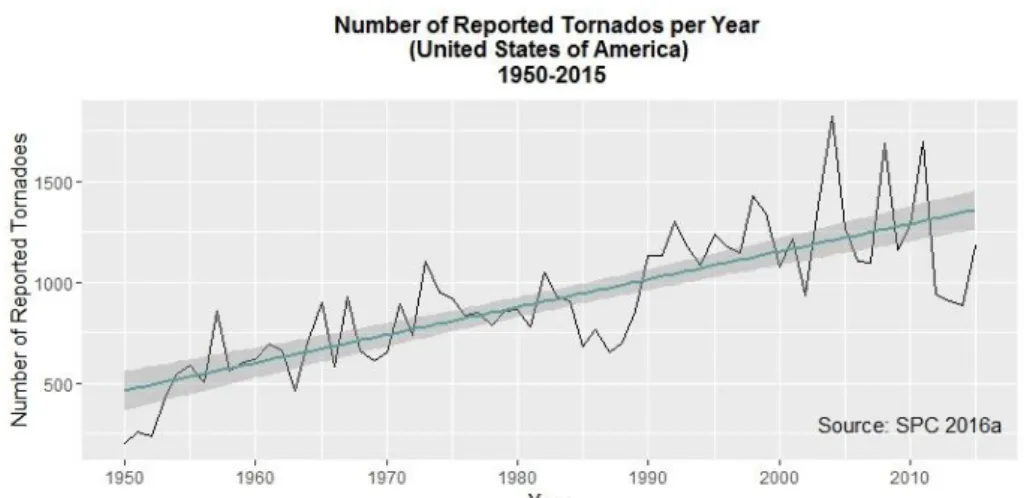
USA are prone to tornado occurrence, leading the list of highest annual tornado counts per country, with an outstanding average value of more than 1000 tornados recorded (after 1990) as denoted by Figure 1-1 (SPC 2016a). The following country in that very same list is Canada, with a much lesser annual tornado counts value: around 100 per year (NCEI 2016a).
Figure 1-1. Evolution of absolute tornado yearly counts in USA, during the period of 1950-2015; The linear smoother denotes the main tendency over the years. Data Source: SPC 2016a. After the heat waves in the last 10 years, tornados are the deadliest natural weather disasters in the United States (Romanic et al. 2016). And, even though each single tornado do not surpass the damage of a hurricane, the sum of losses in property and human lives that all the tornados can cause in a year in the country are very superior to the hurricane ones. Every year, in average, 60 people die from tornado occurrence, 1500 are injured and the losses sum up to 200 million dollars in damage (SPC 2016a).
1.1
Tornado Dataset: some statistics and remarks
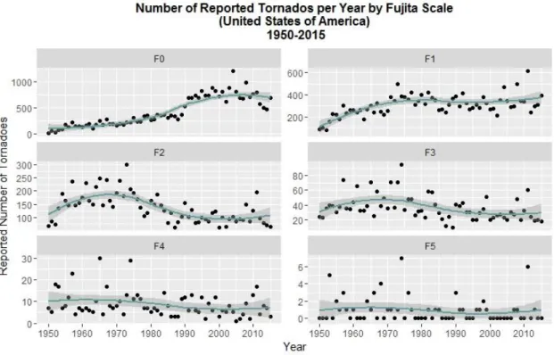
Figure 1-2 shows the number of reported tornados, per Fujita Scale, during the time period comprehended between 1950-2015.
As a side note, Fujita Scale was developed by Theodoro Fujita (1971). Briefly, it organizes tornados by classes of damage, where the designation F0, F1, F2, F3, F4 and F5 are given to the classes “Light Damage”, “Moderate Damage”, “Considerable Damage”, “Severe Damage”, “Devastating Damage” and “Incredible Damage”, respectively. Table 1.1. displays some more detailed information about each damage class.
From simple observation of the plots on Figure 1-1 and 1-2, one can simply assume that the main trend in tornado occurrence in the United States of America is generally increasing with
time. More specifically, tornados from classes F0 and F1, after 1990, presented more registries.
Classes F2 and F3 are more irregular over time, with both having more incidence over the period 1950-1980, and remaining relatively constant until the present.
Table 1-1. Details on Fujita Damage Scale; Damage description from Fujita (1971) and SPC (2016b).
Class F4 is relatively constant through time, with mean values around 10 counts per year; and class F5 occurrence is reserved for only a few years, with a maximum of 6 tornados occurrences in 1974. There are some constrains in what concerns to this postulation, which will be discussed in more detail in Section 4.1.1., but as for now, the main idea is the fact that, as a major trend, tornado occurrence in United States is increasing over time. Even though this rate is more accentuated for the less harmful FS classes, it is worth to remark that even an F0-class tornado could already cause some damage (Table 1.1).
Figure 1-3 displays the annual total of losses in property, total fatalities, and injuries, per year in USA, consequent from tornado occurence.
It is important to point out that the methods to calculate property loss and input the values into the database were very much limited, prior to 1996; for each tornado, there was an attribution of property loss code, whose meanings are presented in Table 1.2. As observable, the thresholds are not, at all, proportional in their increment rate. Therefore, for representation on Figure 1-3, the mean value for each threshold was attributed to each year, to have an approximated mean of comparison with the values after 1996. Yet, this is only a very Scale
Wind Estimate (Km h-1)
Damage (Fujita 1971; SPC 2016b)
F0 <117 Some damage in chimneys, and antennas; some breaks in trees branches; shallow trees pushed over; sign boards damaged.
F1 117 – 180 Surfaces peeled off the roofs; windows broken; light trailer houses pushed; some trees uprooted; moving automobiles pushed off the road.
F2 182 – 253 Roofs torn off frame houses; weak buildings are demolished; trailer houses destroyed; large trees uprooted; light object missiles generated; cars lifted off ground.
F3 254 – 332 Roofs and some walls torn off from well-constructed houses; trains overturned; some rural buildings completely destroyed; most trees in a forest uprooted, snapped or leveled; heavy cars lifted off the ground.
F4 333 – 418 Well-constructed houses leveled, leaving piles of debris; structures with weaker foundation blown away some distance; cars and trains thrown and/or roll for considerable distances; large missiles generated.
F5 419 – 592 Strong frame houses leveled off foundations and swept away; steel-reinforced concrete structures badly damaged; automobile-sized missiles generated and fly through the air for more than a hundred meters; “Incredible phenomena will occur”.
Figure 1-2. Absolute year counts of tornados per year, per Fujita scale. The trend line, computed by ´loess´ method, shows the general tendency for the mentioned period. Data Source: SPC 2016a. unpolished approximation: e.g., if a code 4 is describing the property loss of a tornado, it could be any value between 5 000 and 50 000 dollars, but for the year summation computed for Figure 1-3, a value of 22 500 dollars was inputted. Moreover, analyzing the trends of property losses in dollars, without taking into consideration any inflation and wealth adjustments could lead to what Brooks and Doswell (2000) call as a “temporal myopia”. In their study, they realized that the measurements of property loss in dollars subsequent from
tornados are not increasing over the years, but they reflect the changes in inflation and population wealth.
Nonetheless, even with this rough approximation, after the time of publication of the referred study, it can be assumed a general trend that reflects a yearly increase in property losses. This trend is also clearly accentuated by the 2011 Tornado Outbreak2, with an astonishing value of almost 9 billion dollars in property losses, across the states of Mississippi, Alabama, Georgia, Tennessee, and Virginia (Knupp et al. 2014).
In fact, Figure 1-1 points displays at least 3 years after 2000 where records were broken in what concerns to absolute annual tornado counts (2004 – 1817 tornado counts; 2011 – 1691 tornado counts; 2008 – 1688 tornado counts).
2
Out of curiosity, accordingly to NOAA (2016), 2011 was an unusual year, with some of the deadliest and destructive tornados ever registered (e.g. Joplin in Missouri (SPC 2016c)) and the second year with most registered tornados, with a total of 1691. Several records were broken, including the more number of tornados in a single month (758 in April) and the greatest daily total (200, on April 27th).
Regarding the evolution of fatalities over the time, there is a general decreasing trend over the period of 1950 to 1990, from 150 annual deaths to 50, a value that raises until the present day to an average to 150 deaths. It is worthy to point out that what seems to be an accentuated increase over the last 15 years, is highly dictated by the extreme values of 2011.So, having this fact into consideration, the apparent increase can be explained partially by the fact that the tornado occurrences are raising over time, and partially by the fact that, as the time increases, the accuracy of registries become more accurate, due to improvements in technology, measurement devices, etc.
The number of injuries seem to, after 1975, follow a general decrease over time, even though there are some outliers from the general tendency that express extreme values. These extreme values are scattered among time, and represent extremely high values.
Under these statements, two scenarios can be assumed to interpretation of Figure 1-3: either property losses, injuries and deaths subsequent from tornados are increasing over time, since 1950; or, in a more skeptical view, they have been remaining constant over the years (in what concerns to median values), and external factors to the database are creating an illusion of increment (including social and economic factors) as well as internal factors (tornado classification methods; property losses classification methods; machine-based spotting of events, such as radar, that could have misinterpretations).
Table 1-2. Codes attributed at the tornado database (SPC 2016a) to characterize consequential property loss from each tornado
From 1950 to the present time, technology advanced and developed at an exponential rate, improving both forecasting methods and the disaster response strategy. In this sense, it would be expected that the social and economic consequences of tornados would represent a general decrease over time, which, in both scenarios, do not appear to be the most feasible option. As a wrap-up from all this information, the conclusion to reach is that the changes on how tornados are reported make it difficult to formulize a general trend. But, as pinpointed by Brooks et al. (2014), one fact is for sure: the variability of occurrence has increased since the 1970s, given the standard deviations, and for the last years, several extreme events have been reported. Tippet (2014) endorses the theory of increasing variability by reporting an increase
Code Threshold of Property Losses in Dollars
1 < 50 2 50 – 500 3 500 – 5 000 4 5 000 – 50 000 5 50 000 – 500 000 6 500 000 – 5 000 000 7 5 000 000 – 50 000 000 8 50 000 000 – 500 000 000 9 > 500 000 000
in the volatility of annual tornado frequency, given by the standard deviation of the difference between annual tornado counts of consequent years.
On the other hand, in what concerns to the formulation of a generalized trend, the studies made so far reflect a vast heterogeneity. On one side, some studies have shown that the annual number of tornados in US have not increased over time, e.g. Brooks et al. (2014); Elsner et al. (2015); Tippett and Cohen (2016). On the other hand, there are studies that support the thesis that they are increasing (Gensini and Mote 2015; Seely and Romps 2015; Tippet et al. 2015).
From another perspective, Tippet and Cohen (2016) report a growing trend of the mean of number of tornados per outbreak per year.
Figure 1-3. Annual Totals of Property Losses, Fatalities and Injuries, subsequent of tornados, during the period of 1950-2015 (Data Source: SPC 2016a)
1.2 The Tornado Alley
Under the thematic of USA tornado sensitivity, presented over the last paragraphs, there is a zone in the United States, nicknamed by the media as Tornado Alley zone (NSSL 2016). Bibliography varies in what concerns to which states belong to this area or not, e.g., in
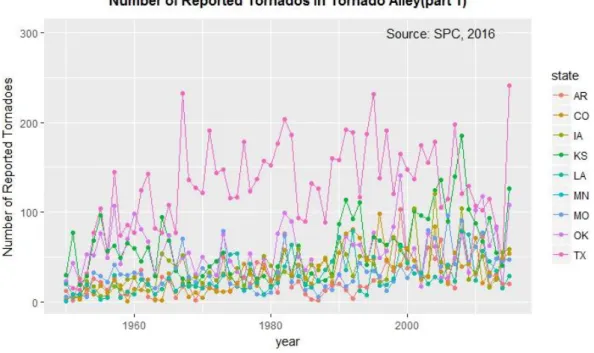
Tornado (2017), Concannon et al. (2000) or Scolastic (2017); Coleman and Dixon (2014) present a great discussion about this matter. The difference of definition of this zone lies in the difference for quantification of tornados, as it could be expressed in many different ways: by all tornado counts, by tornado-county segments, or strong and violent tornados only (NSSL 2016). For the scope and purpose of this thesis, the following states were considered as inside the Tornado Alley Region (Figure 1-4.): Oklahoma, Kansas, Arkansas, Iowa, Missouri, Texas, Colorado, Louisiana, Minnesota, South Dakota, Mississippi, Illinois, Indiana, Nebraska, Tennessee, Kentucky and Wisconsin.
Figure 1-4. States that compose the Tornado Alley zone, or, in other words, states that have major incidence of tornado records in USA.
Figure 1-5 shows the yearly counts of tornados for each of the states of the referred zone. From all, Texas is the state that, by far, has more incidence of tornado occurrence, followed by Oklahoma and Kansas. All the other states follow, more or less the same trend, in tornado counts inside the threshold of 0-100 tornados year -1.
1.3 Why so many tornados?
The physical and meteorological principles behind the great occurrence of tornados in the USA at the national level is well studied and understood (Jagger et al. 2015). As Brooks (2014) and Grazulis (2003) explain, the central US are the place where tornados are more likely to occur, due to the presence of the Rocky Mountains and the Gulf of Mexico. “The
surface winds from the south bring warm and moist air at low levels, whereas the winds from the west bring upward relatively cold and dry air, forming a north-south barrier.The temperature and moisture profile brings in the right conditions for thunderstorms and the change of the wind with height means storms will rotate” – Brooks (2014).
This has more influence during the spring, across Oklahoma and Kansas (Schultz et al. 2014) and will spread towards north to the northern Plains and Midwest during summer, due to the migration of the jetstream northwards (Brooks and Doswell 2000; Jagger et al. 2015).
Nonetheless, the regional-scale dynamics is poorly understood (Jagger et al. 2015). This is due to several facts.
Figure 1-5. Number of absolute counts of tornados per year, for all states of the Tornado Alley3. Data Source: SPC (2016a)
Firstly, tornado events are locally rare, discrete and mostly clustered. Moreover, the quality for tornado records is uneven. The tornado national database for the United States, even though the biggest in the world, with records from 1950 to nowadays, it has many issues in what concerns to data interpretation for climatic studies, as referenced by countless studies,
3States Acronyms: “AR” – Arkansas; “CO” – Colorado; “IA” – Iowa; “KS” – Kansas; “LA” – Louisiana; “MN” –
Minnesota; “MO” – Missouri; “OK” – Oklahoma; “TX” – Texas; “IL”- Illinois; “IN” – Indiana; “KY” – Kentucky; “MS” – Mississippi; “NE” – Nebraska; “SD” – South Dakota; “TN” – Tennessee; “WI” – Wisconsin.
e.g., Verbout et al. (2006), Doswell (2007), Coleman et al. (2011), Elsner et al. (2013), Kunkel et al. (2013), Widen et al. (2013), and Elsner et al. (2016)4.
1.4 Final Problem Statement
USA are highly prone to tornados and this tendency seems to be increasing over time, as shown above. Not only the tendency of tornado occurrence seems to be increasing, but also, over the last decade, the extreme events, with tornado counts superior to 1500 tornados per year in the USA, values that were never reached before.
Tornados are a big source of property loss, injuries, and even fatalities; they can devastate huge zones, leaving nothing behind but destruction.
The physical climatology is well studied at the national level, but not so well for the regional scale (Jagger et al. 2015). In this sense, modelling tornado occurrence at the regional scale could help to better understand what are the mechanisms that favor tornadogenesis. This, in turn, could lead to serious improvements in what concerns to disaster management and response. Namely, a model that specifies the occurrence of tornado counts as a function of several covariates, characteristics of a given place, and that also has into consideration the spatial and temporal components (Moore 2017). Moreover, if defined at the county-level for a determined state, it could be of great interest to local authorities to improve both prevention and response to tornadoes. Furthermore, if it is clear what are the mechanisms that can control tornadogenesis for a county, the design of tornado-county alert, and risk zones alerts will be much more effective and precise. In this sense, it is also possible to understand on how a change in the territory could enhance or reduce the risk of tornados. Thus, such a model will not only help local policies in what concerns to disaster management and response, but also in what concerns to land management: e.g. in construction site definition or environmental management.
1.5 Objectives
Once Texas is the state in the Tornado Alley that has more occurrence of tornados, the main objective is to model spatio-temporal tornado occurrence at the county level for this state. The modelling strategy has into consideration three covariates: Elevation, Population and Land-Cover. Beyond the covariates, the model should have into consideration the spatial and temporal variability. The model is then tested against Oklahoma, the second state out of all 50 states that have more tornado occurrence.
The study focus is mainly concentrated on understanding how tornados are distributed over space and time, at the county level for Texas, and the potential link between tornado occurrence and the above mentioned covariates, using two approaches: point processes and lattice. The first one will take into consideration each single tornado occurrence. The second one takes into consideration the amount of tornados at the county level, per year, from 1970 to 2015. For Oklahoma only the lattice approach will be performed to attest the quality of the state-based tornado model.
1.6 Research Questions
The main research questions for this study are:
Would it be possible to come up with a reliable regional scale (for a state at the county level) model from a scattered and apparently non-reliable database?
What is the spatial and spatio-temporal distribution of tornado occurrence in Texas?
Are the events clustered somehow?
Is there any link between the tornado occurrence and the terrain roughness?
Is there any link between the tornado occurrence and population of a place?
Is there any link between tornado occurrence and different kinds of land-cover classes?
What is the statistical model equation that defines the spatial and temporal structure of tornado occurrence per state in Texas?
What is the final statistical model equation that better describe tornado occurrence in Texas?
Does this model fits another state?
1.7 Thesis Structure
In order to follow the reproducible research principle, all scripts (R and Arcpy) and data are given at https://github.com/AngRodrigues/Modelling-Tornado-Ocurrence-with-R-INLA. For future reference, the coordinate reference system used for the whole geoprocessing and statistical analysis was the EPSG 102003, which is the Conic Contiguous Albers Equal Area projection for USA.
The second chapter deals with the theoretical framework, that gives an overview of the general principles applied in this thesis, from Bayesian statistics, to the R-INLA principles and spatio-temporal modelling within its framework. It also gives a «n overview of past research that had as an objective the tornado occurrence modelling.
Chapter three presents the study areas, Texas and Oklahoma, and gives a general overview of the distribution of occurrence of tornados in those states.
Chapter four refers to the resources used, from data (with a description of each dataset) to the software.
Chapter five presents all the steps used in the data analysis, and some complements on the theoretical framework, related to the model specifics.
Chapter six shows the results and discussion, and chapter seven highlights the main conclusions.
Bibliography is presented in chapter 8, and chapter 9 has all the attachments.
2.
THEORETICAL FRAMEWORK
2.1 Bayesian Framework
During the last three decades, Bayesian methods have been suffering significant advances and are starting to be extensively recognized in many investigation areas (Blangiardo et al., 2012).
2.1.1 Bayesian Statistics
Bayesian statistics have a huge influence from conditional probability, as well documented and discussed by Hartmann and Sprenger (2010) and Hajek and Hartmann (2010), and even more detailed in Samandiego (2010) and Wakefield (2013). Bayes theorem (Bayes and Price 1763) is defined as:
P B A = P A B ∗ P (B) P(A)
In simpler words, the theorem follows the ideas developed by Bayes and Laplace regarding inverse probability: the probability of an event B, given that an event A occurs. So, it all occurs following the process: P(B) is computed before the event A is observed; then the P(A) is computed and used to access the P(B) and P(B|A) is then accessed.
In this sense, P(A) is the information on the event of interest available a priori, without carrying any experiment (also called prior information); this probability will affect the posterior probability of B. Thus, the P(B) will be dictated both by the prior information, as well as by the results of the experiment itself (Blangiardo and Cameletti 2015).
2.1.2 Bayesian Inference
Bayes theorem is well established in what concerns to observable events. But when it comes to Bayesian inference, i.e., general statistical analyses, where the parameters are less-known quantities and their prior distribution needs to be specified in order to reach the posterior distribution, its application becomes more controversial (Blangiardo and Cameletto 2015).
Let a random variable be Y, and the data available for its analysis be 𝑦 = (y1, … , yn)’. Its uncertainty is modeled using a probability function or a density function (for a discrete or continuous variable, respectively) which is always indexed by a parameter θ. The likelihood function 𝐿 𝜃 = 𝑝 𝑌 = 𝑦 𝜃 , or, simpler, 𝑝(𝑦|𝜃), specifies the distribution of the data y under the model defined by 𝜃.
The variability on 𝑦 depends on the sampling selection: it is assumed that the data are a random sample from the study population and uncertainty is generated by the fact that we only observe that sample instead of all the possible other ones (Blangiardo and Cameletti 2015).
The parameter 𝜃 is modeled through a suitable prior probability distribution 𝑝(𝜃), before any observation of a realization 𝑦. Given the two components, prior and likelihood, the inferential problem is solved by recurring to Bayes Theorem, to obtain the posterior distribution – 𝑝(𝜃|𝑦) - which represents the uncertainty about the parameter θ after observing the data:
p θ y = p y θ ∙ p(θ) p(y)
The denominator 𝑝(𝑦) defines the marginal distribution of 𝑦, or the “prior predictive distribution of 𝑦” (Jeffreys 1961), is defined as:
p y = p y θ p θ d θ
and indicates what y should look like, given the model, before y has been observed (Statisticat LLC 2015); it is considered a normalization constant, so the Bayes theorem is also reported as:
p(θ|y) ∝ p(y|θ) × p(θ)
In other words, the posterior distribution is proportional to the likelihood times the prior distribution, known as the “Bayesian Mantra” (Jackman 2009).
2.1.3 R-INLA: The Integrated Nested Laplace Approximation
2.1.3.1 The Algorithm
INLA algorithm was introduced by Rue et al. (2009). It is a deterministic algorithm for Bayesian inference. This is the key-point that makes it different from Monte Carlo and Markov Chain Monte-Carlo, because these are based in simulations. INLA is specially developed for latent Gaussian models and provides accurate results for an improved computing time, when compared to MCMC (Blangiardo and Cameletti, 2015). LGM‟s, or structure additive regression models, are a widely used class of models in statistical applications (Rue 2014). They include, amongst others, generalized linear models, smoothing
spline models, spatio and spatio-temporal models, log Gaussian Cox-processes and geostatistical and geo-additive models (Rue et al. 2009).
The very first step to define a latent Gaussian model within the Bayesian framework is to identify a distribution for the observed data 𝑦 = (𝑦1, … , 𝑦𝑛). As a general approach, it is specified a distribution for 𝑦𝑖 characterized by a parameter 𝜙𝑖. This parameter is given by a function of a structured additive predictor 𝜂𝑖 through a link function f(⋅), such that 𝑓(𝜙𝑖) = 𝜂𝑖. In this sense, the additive linear predictor 𝜂𝑖 is given by:
𝜂𝑖 = 𝛽0+ 𝛽𝑚𝑥𝑚𝑖 + 𝑓𝑙(𝑧𝑙𝑖) 𝐿 𝐼=1 𝑀 𝑚 =1 Where:
𝛽0 is a scalar representing the intercept;
the coefficients 𝜷= {𝛽1,… , 𝛽m} quantify the (linear) effect of some covariates
x=(x1,…,xm) on the response;
f = {f1(⋅),… , fL(⋅)} is a collection of functions defined in terms of a set of covariates
z=(z1,… , zL).
The terms fl(⋅) can assume different forms such as smooth and nonlinear effects of covariates,
time trends, temporal or spatial random effects. For this reason, the latent Gaussian models can be used in a wide range of applications, from generalized and dynamic linear models, to spatial and spatio-temporal models (Blangiardo and Cameletti, 2015).
In this sense, all latent (non-observable) components of interest are collected, in a set of parameters designated by θ (θ = {𝛽0, β, f}. In addition, it is needed to specify a vector K of
hyperparameters such as 𝜓= {𝜓1, … , 𝜓K}.
By assuming conditional independence, the distribution of n observations is given by a likelihood:
𝑝 𝑦 𝜃, 𝜓 = 𝑝 (𝑦𝑖|𝜃𝑖, 𝜓 𝑛
𝑖=1
)
Where each data point yi is connected to one element θi in the latent field θ.
On the logarithm, it is assumed a multivariate normal prior on θ, with mean 0, and precision matrix Q(𝝍), i.e., 𝜽∼ Normal(𝟎, Q−1(𝝍)) with density function given by:
𝑝 𝜃 𝜓 = (2𝜋)−𝑛2 |𝑄 𝜓 1 2exp 1
2𝜃′𝑄 𝜓 𝜃
This specification is known as Gaussian Markov random field, where the components of the latent Gaussian field 𝜽are supposed to be conditionally independent with the consequence that Q(𝝍) is a sparse precision matrix.
The specification matrix is what improves computational times (Blangiardo and Cameletti, 2015). Here, the joint posterior distribution of 𝜽 and 𝝍 is given by:
𝑝 𝜃, 𝜓 𝑦) ∝ 𝑝 𝜓 ∙ 𝑝 𝜃 𝜓 ∙ 𝑝(𝑦|𝜃, 𝜓) ∝ 𝑝 𝜓 ∙ 𝑝 𝜃 𝜓 ∙ 𝑝(𝑦𝑖|𝜃𝑖, 𝜓 𝑛 𝑖=1 ) ∝ 𝑝 𝜓 ∙ |𝑄 𝜓 |1/2exp −1 2𝜃′𝑄(𝜓)𝜃 ∙ exp log 𝑝 𝑦𝑖 𝜃𝑖, 𝜓 𝑛 𝑖=1 ∝ 𝑝 𝜓 ∙ 𝑄 𝜓 12exp −1 2𝜃′𝑄 𝜓 𝜃 + log(𝑝 𝑦𝑖 𝜃𝑖, 𝜓 ) 𝑛 𝑖=1
Under the scope of R-INLA, the objectives of Bayesian inference are the marginal posterior distributions of each element of the parameter vector
𝑝 𝜃𝑖 𝑦 = 𝑝(𝜃𝑖, 𝜓 𝑦 ∙ 𝑑𝜓 = 𝑝 𝜃𝑖 𝜓, 𝑦 ∙ 𝑝 𝜓 𝑦 ∙ 𝑑𝜓
And also for each element of the hyperparameter vector,
𝑝 𝜓𝑘 𝑦) = 𝑝 𝜓 𝑦) 𝑑𝜓−𝑘
In this sense, two tasks are needed to achieve:
the computation of p(𝜓|y), from which also all the relevant marginals p(𝜓𝑘|y) can be
obtained;
the computation of p(𝜃i| 𝜓, y), which is needed to compute the parameter marginal posteriors p(𝜃i|y).
The idea to maintain here is that R-INLA perform these two tasks. The details on how they are processed and approached mathematically and computationally are given in Rue et al. (2009).
In this sense, “eff ectively only one form of uncertainty exists, which is described by suitable probability distributions” (Blangiardo et al. 2012). Consequently, there is no difference between observable data or unobservable parameters; these are also considered as random quantities. Under the Bayesian framework, the uncertainty about the realized value of the parameters given the current state of information (i.e. before observing any new data) is described by a prior distribution. Typically, but not constantly, the objective of the inference
is to deliver the posterior distribution; the inferential process, thus, combines the prior and the data model itself to derive the posterior distribution (Lindley, 2006; Blangiardo et al. 2012).
2.1.4 Spatio-temporal modelling under the Bayesian Framework
R-INLA has been used for an infinity of applications. Here are presented some recent studies that used INLA spatio-temporal capabilities:
Laurini (2017) recurred to INLA to analyze the spatio-temporal gasoline price, arriving to a contiguous space model that allows the estimation of prices distribution throughout Brazil.
Wang et al. (2017) estimated car crashes by crash types and crash severity, having into consideration factors such as crash type and severity counts on rural two lane highways.
Braulio-Gonzalo et al. (2017) model the energy performance and indoor thermal comfort of residential stocks at a city-scale.
Diaz-Avalos et al. (2016) modelled the wild fires in Castellón, Spain, for the period of 2001-06, using several spatial covariate information, in order to predict and, therefore, prevent wildfires in the zone.
Tabb et al. (2016) modelled the relationship between alcohol outlets availability and violence, for the period of 2010-2013, in Seattle, USA.
Breivik et al. (2017) used the INLA process to model historical bycatch in commercial fisheries, and project a prediction for the future.
The reason why many studies take advantage of the R-INLA, instead of other tools, is the computational time; MCMC takes days to compute, while INLA takes a few minutes. Moreover, there are advantages related to the modelling approach itself are quite something. For example, the specification of prior distributions allows the formal inclusion of information that can be obtained from previous studies or from expert opinion. In addition, the (posterior) probability that a parameter does/does not exceed a certain threshold is easily obtained from the posterior distribution, providing a more intuitive and interpretable quantity than a frequentist p-value (Blangiardo et al. 2012).
In addition, and perhaps the most important fact, is that, within the Bayesian approach, it possible to postulate a hierarchical structure on the data and/or parameters, which presents the added benefit of making prediction for new observations and missing data imputation relatively straightforward.
Theoretically, data that contains a spatial component are the so well-known spatial data, and are defined as a realization of a stochastic process indexed by space
𝑌 𝑠 ≡ { 𝑦 𝑠 , 𝑠 ∈ 𝐷} where D is a fixed subset of ℝd
(Rue et al. 2009).
In what concerns to spatial data, Cressie (1993) and others, such as Gelfand et al. (2010), grounded and structured the distinction between three types of spatial data: Area (or lattice) data; point referenced (or geostatistical) data; and spatial point patterns.
Spatial data is considered by many as a “special kind of data”, considering that the spatial trend has to be taken into consideration for its interpretation. The spatial component will provide such an additional information that, if neglected, could lead to serious biases in estimations. Under this scope, the Bayesian approach is particularly effective (Blangiardo et al. 2013; Gómez-Rubio et al. 2014; Bivand et al. 2015; Blangiardo and Cameletti 2015). All above mentioned types of spatial data can be fitted into models, under the Bayesian framework, by extending the concept of hierarchical structure; such structure will acknowledge similarities that are based on the neighborhood or on the distance (Blangiardo and Cameletti 2015). For the purpose and scope of this thesis, area data will be explored under the Bayesian framework. For details on the other two types of spatial data, please see Blangiardo and Cameletti (2015).
At the area level of data, the neighbor structure dictates the spatial dependency. Given the area i, its neighbors N(i) are specified as the areas that share borders with it (first order neighbors), or that share border with its first order neighbors. Under the Markovian property that the parameter θi for the ith area is independent of all the other parameters, given the set of
N(i) (local Markov property), then
𝜃𝑖⊥⊥ 𝜃−𝑖 | 𝜃𝑁 𝑖
Where θ-i indicates all elements in the parameter θ, except the ith. In this sense, the precision
matrix Q of θ is sparse, a fact that enhances computational benefits. Thus, for any pair of elements (i, j) in θ
𝜃𝑖⊥⊥ 𝜃𝑗 | 𝜃−𝑖𝑗 ↔ 𝑄𝑖𝑗 = 0
Meaning that the precision matrix is now given by the neighbor structure of the event, by the pairwise Markov property. Qij ≠ 0, only if j∈ {i, N(i)}. The independence of θi from θj is not
only conditioned by the hyperparameters, but also by the set of neighbors. The main formulation is specified in
The precision matrix can be now specified as a function of the structure matrix, as well documented by Rue and Held (2015):
𝑄 = 𝜏 𝑅 Where
𝑅𝑖𝑗 =
𝑁 𝑖 , 𝑖𝑓 𝑖 = 𝑗 1, 𝑖𝑓 𝑖 ~ 𝑗 0, 𝑜𝑡𝑒𝑟𝑤𝑖𝑠𝑒
Where i ~ j denotes that areas i and j are neighbors.
The spatial framework described does not allow to characterize the temporal variation of the data; it should be extended to the spatio-temporal case, by including a time dimension. Thus, both spatial and temporal models can be incorporated into a unique model to enhance the detection resolution. In a prior instance, the stochastic models were designed to, mainly, define a temporal model on a pixel, and, having it into consideration, subsequently describe the spatial model, as described by, for example, Ahmad and Collet (2016), or Friston et al. (1994).
Bayesian models are a reflection of this technique (Craigmile and Guttorp 2011). In this sense, data should be defined by a process indexed by space and time:
𝑌 𝑠, 𝑡 ≡ 𝑦 𝑠, 𝑡 , 𝑠, 𝑡 ∈ 𝐷 ⊂ ℝ2 ∙ ℝ
That are observed at n spatial areas and at T time points.
More details in what concerns spatio-temporal model are given in section 5.2.4.
2.2 Modelling Tornado Occurrence
Literature in this matter is extensive. On one side, because of the above cited USA‟s tornado occurrence susceptibility. Secondly, because modelling techniques are different amongst the different studies and the study region scale largely varies from study to study.
The National Center for Environmental Information (NCEI) and Storm Prediction Center (SPC), included in the National Oceanic and Atmospheric Administration (NOAA), are the main suppliers for tornado information in USA (e.g. NCEI 2016a;NCEI 2016b; SPC 2016a). Data provided by this information center was the basis of inspiration for many studies that make an attempt to theoretically explain, model and forecast tornado occurrence in the USA (e.g. Boruff 2003; Ashley et al. 2008; Dixon et al. 2011; Dixon and Moore. 2012; Widen et al. 2013; Ashley et al. 2014; Coleman and Dixon 2014; Cusack 2014; Rosecrants and Ashley 2015; Elsner et al. 2016; Romanic et al. 2016; Moore 2017), to name a few.
Beyond these studies, there were over the last years, many authors that tried to compute statistical models to describe tornado occurrence. Here is a compilation of some of the methods and models proposed:
Wikle and Anderson (2003) came up with a spatio temporal model constructed under the Bayesian framework, based on tornado count data for USA. In this study, it was used a zero-inflated Poisson likelihood to model the excess of zeros; the mean of this Poisson is then
modelled using different spatial and non-spatial random effects; a relationship with the El Niño/Southern Oscillation phenomenon was also taken into consideration.
Elsner et al. (2013) built a model to predict violent tornados during springtime across US Central Plain, as a function of the nearest distance to a Poisson point process of non-violent tornados. It was also proposed a correction for the population bias (which they assume is expressed by less tornado reports in less populated areas), by including the distance to the nearest city.
Karpman et al. (2013) suggested some spatio-temporal models, that were implemented by using an approach that is based on non-parametric kernel. The variables used in the model were tornado point patterns and topographic variation. The model was selected recurring to AIC5.
Elsner et al. (2014) proposed a model where tornado intensity is assumed to be distributed as a Weibull with the log-mean depending linearly on the path length and width which are strongly correlated to the Fujita categories.
Akers et al. (2014) also explored the relationship between length and width of tornados and intensity, by recurring to a multinomial logistical model, without spatial random effects, to compute the probability of a particular tornado with a certain FS class occur.
Gomez-Rubio et al. (2015) analyze the dataset by performing a model under INLA framework and estimated with stochastic Partial Differential Equations, to model the intensity of point patterns with marks.
Jagger et al. (2015) proposed a regional scale model, that assumes a negative binomial distribution for tornado occurrence and is normalized with population, and has into account fluctuations in elevation and CWA.
3 STUDY AREA
3.1 Texas
Texas is the more southward state of USA, Figure 3-1. Toponymically, the word Texas was the Spanish pronunciation of Tejas. The latter was the Hasinai Indian word for allies or
friends. Their state motto is, in fact, “friendship” (Dingus 1981).
Texas is the second most populous state in US, after California. This state has three of the top ten most populous cities in the USA, which are Houston, Dallas, and San Antonio, and 70% of its population lives within 200 miles of Austin, the capital of the state (USCB, 2016).
5 Refer to section 5.2.
It covers 7.4% of the total USA‟s area, with around 80% of its own land being covered by farms, and 10% covered by forest, a class that includes four national and five state forests (USGS 2014d).
The highest point of Texas is the Guadalupe Peak, at 8749 feet and the lowest is the Gulf of Mexico (USGS 2016).
The deadliest natural disaster in this state, that there are records of, was Galveston Hurricane, in 1900, which killed around 8 000 to 12 000 people (Dar, 2008).
Figure 3-1. Location of Texas in USA, with representation of main cities, and surrounding states.
Out of all states that were considered as belonging to the well-known Tornado Alley,
Texas is the one that has major tornado counts over the years (Figure 1-5.). In fact, it
is the state in USA that has more tornado counts per year. Of course, this statement is
largely biased by the fact that Texas covers, after Alaska, the greatest area, out of all
the 49 states.
Texas is shared by two areas that are potentially prone to tornado occurrence: the
already referred “Tornado Alley”, reserved to the central plains of the US, and “Dixie
Alley”, which has its main concentration in states across the Gulf of Mexico. These
zones are highly prone to tornado occurrence. This fact occurs because they constitute
the meeting point of the humid air from the Gulf of Mexico, hot dry air from Arizona
and New Mexico, and cool dry air from Canada. Specially in spring time, these
masses of air work together and originate most of tornados.
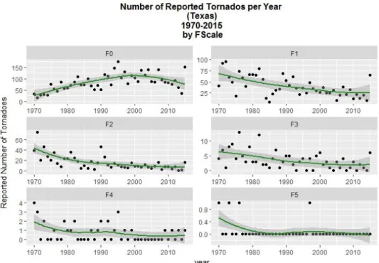
Figure 3-2 shows the year tornado counts for Texas, per FS, over the period of
1970-2015
6(Source SPC 2016a). It is clear that F0 tornados are the ones with more
prevalence, with mean values generally above 75 counts per year; classes F1, F2 and
F3 seem to follow a decreasing trend after the seventies and eighties, the very same
period where F0 tornado counts seem to increase. This could be related to the
aforementioned fragility of the database. What is worth to pinpoint is that weaker
tornados occur more than stronger ones: F4 tornados fluctuate over time, but never get
over the limit of four tornados per year, and, after 2010, there is one event every two
years. F5 tornados are considerably rare in Texas.
Figure 3-2. Number of tornado reports in Texas, over the period from 1970 to 2015, represented by FScale, with trend line computed by “loess” method. Source SPC 2016a.
Figure 3-3 displays the total number of tornado counts per county in Texas, over the
period of 1970-2015. There are several counties with a minimum value of two tornado
counts over the years. The county that has more total tornado counts over the years is
Harris, with 189 tornados, followed by Hale and Galvinson, with 85 and 80,
respectively. The mean value of total tornado counts is the summation of 26 tornados.
3.2 Oklahoma
Oklahoma is the state that is immediately northwards Texas. It covers around 180 000 Km-2 of American soil, being the twentieth biggest in area. With a population of 3 700 000 inhabitants, it is the second state that has more native American population.
In what regards to tornados, Figure 3-4. shows the tornado yearly tornado counts per FScale. As mentioned before, Oklahoma is the second state in the Tornado Alley with more occurrence of tornados per year. The distribution for each FS class follows, generically, the same as Texas, with an occurrence trend that decreases with increase in FS. Nonetheless, is worth to pin-point the great increase of F0 and F1 tornados after 1990. From the observation of Figure 3-5., the states that had a major occurrence of tornados during the period 1970 to 2015, have a total count of around 80, a much smaller value than the ones for Texas.
Figure 3-3. Map of Texas with the number of tornados per county during the period 1970-2015. Please note that these values are the summation of tornado reports of all years.
Figure 3-4. Number of tornado reports in Oklahoma, over the period from 1970 to 2015, represented by FScale, with trend line computed by “loess” method. Source SPC 2016a.
Figure 3-5. Map of Oklahoma with the number of tornados per county during the period 1970-2015. Please note that these values are the summation of tornado reports of all years.
4.1 Data description
4.1.1 Tornado Occurrence in North-America
The tornado database used for this study is provided by the Storm Prediction Center, from the National Oceanic and Atmospheric Administration of USA (SPC 2016a). It was originally organized by the SPC, from newspaper accounts and reports (Corfidi 1999; Schaefer and Edwards 1999).
Generally, the database contains records from tornados that occurred in USA since 1950 until the present time. For each tornado are recorded several attributes, from time and date, to state, losses amount (for crops and property), magnitude, length, width, injuries, fatalities, among others. This specificity of data allows an infinity of different combination of space, time and attributes, originating a multitude of kind of analysis: from point processes to lattice data; at national, state, or county level; hourly, weekly, seasonal, monthly or yearly approaches; by attribute (FS, damage, etc.). Though the high specificity of the database, it has several limitations that many authors have been pointing out.
It all comes down to a simple limitation: the fact that the tornado records rely mostly on visual spotting and human annotation of occurrences. From this fact,
Hart (1993) was one of the many authors that reported the fact that the number of reports are greater for places or regions with a greater population density. Therefore, factors such as highways distribution or distance to an official reporting station can influence the numbers is the database.
The occurrence of F0 and F1 tornados shows a dramatic increase since 1980, while the stronger ones remain steady over time (Figure 1.2.). Otsby (1993) was one of the first authors to realize that reasons for this include an improvement of verification efforts by local offices but also a marked increase in tornado chasing.
Doswell et al. (1999) and Verbout et al. (2006) advocate that due to technological developments and more tornado chasers, the probability of a tornado be reported will increase.
Elsner et al. (2013) adds that the number of tornados reported in the database are smaller than the actual number of occurrences, but that this difference is shrinking over time.
Widen et al. (2013) says that the database is imprecise and inhomogeneous, and that any resulting study from raw data will have a lower estimated risk of encountering a tornado.
In order to minimize some of this limitations, it was followed the advice from SPC not coun the tornados prior to 1970.
Moreover, several authors have been working intensively in this database, especially in what concerns to spatial and spatio-temporal analysis, as presented in section 2.2., and therefore, the database seems to be suitable for the scope of this study, with the temporal correction. In fact, this is one challenge to overcome: the difficulty of uniformizing the database.
4.1.2 Digital Elevation Model
The DEM was retrieved from USGS (2016), with a pixel resolution of 1x1 Km. The same resolution was used throughout data analysis. The two states were clipped from the original dataset. It was needed a data simplification process, due to the high dimensions of each raster file. Therefore, the Topographic Position Index was calculated. It was developed by Weiss (2001) and compares the elevation of each cell in a DEM to the mean elevation of a specified neighborhood around that cell.
In this sense, focal statistics were applied for the 10 adjacent cells of each pixel, and the final equation to compute the TPI was:
𝑇𝑃𝐼 =𝑚𝑒𝑎𝑛𝑟− 𝑚𝑖𝑛𝑟 𝑚𝑎𝑥𝑟− 𝑚𝑖𝑛𝑟
Where mean represents a smoothed DEM, computed by the mean of 10x10 adjacent cells of each pixel, and min and max are the DEM with minimum and maximum values of the 10x10 adjacent cells. The python script used to compute it is shown in Attachment A.1., for the case of Texas. The Oklahoma one followed the same procedure.
Figure 4-1 shows the TPI computed for Texas, and Figure 4-2. the TPI for Oklahoma. The index varies from 0 to 1, with values near 0 representing areas characterized by flat plains, and values close to 1 by peaks and ridges (Seif 2014). This generalization was imperative to simplify the inputted data on INLA, and worked as a simple but effective representation of elevation variability. Then, the standard deviation of this index was used to input in the modelling strategy, once it reflects itself a measure of Terrain Roughness (Riley et al. 1999; Ascione et al. (2008).
Figure 4-1. Topographic Position Index for Texas. Original DEM from USGS 2016.
Figure 4-2. Topographic Position Index for Texas. Original DEM from USGS 2016.
Jagger et al. (2015) uses the same strategy: they represent the Roughness Index as a measure of the standard deviation of elevation.
The new approach in this study is to simplify the DEM with the TPI computation and use its standard deviation as a measure of Terrain Roughness.
4.1.3 Population
Historical Population estimations were retrieved from the NBER (2016) for both states. The data was organized as individual counts per state per year, with a temporal coverage for the
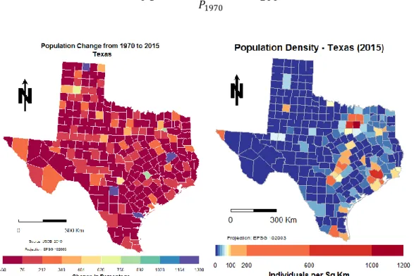
period 1970 to 2015. Figure 4.3. shows the population change in percentage over the study period, for Texas, as well as the most recent population density (2015) and Figure 4.4. shows the population change for Oklahoma, and respective population density, given by:
𝑃𝐶 = (𝑃2015 − 𝑃1970) 𝑃1970 ∙ 100
Figure 4-3. Left: Population Change given by percentage between the years of 2015-1970 for Texas; Right: 2015 Population density for Texas.
It is possible to see that from 1970 to the present day, in Texas, the population of more than half of the counties doubled, at least. The county of Ansford, Houston, Medina and San Patricio show an increase of population in the order of 1300% from the original values of 1970.
In order to account for the difference of area values between the counties, the unit used to input in the models was given by the population density (individuals per square kilometer). Oklahoma shows a smaller percentage of change in the time period, which means that variability for this variable is lower spatially and temporally. The county with the highest percentage of change was Latimer, with 300% of positive change.