Spatio-Temporal Modeling of Data Imputation for Daily Rainfall Series
in Homogeneous Zones
José Ruy Porto De Carvalho, Alan Massaru Nakai, José Eduardo B.A. Monteiro
Embrapa Informática Agropecuária, Campinas, SP Brazil.
Received: 9/3/2015 - Accepted: 17/08/2015
Abstract
Spatio-temporal modelling is an area of increasing importance in which models and methods have often been developed to deal with specific applications. In this study, a spatio-temporal model was used to estimate daily rainfall data. Rainfall records from several weather stations, obtained from the Agritempo system for two climatic homogeneous zones, were used. Rainfall values obtained for two fixed dates (January 1 and May 1, 2012) using the spatio-temporal model were compared with the geostatisticals techniques of ordinary kriging and ordinary cokriging with altitude as auxiliary vari-able. The spatio-temporal model was more than 17% better at producing estimates of daily precipitation compared to kriging and cokriging in the first zone and more than 18% in the second zone. The spatio-temporal model proved to be a versatile technique, adapting to different seasons and dates.
Keywords:spatio-temporal model, rainfall data, ordinary kriging, ordinary cokriging, homogeneous zones.
Modelagem Espaço Temporal para Imputação de Dados para Séries de
Precipitação Diária em Zonas Homogêneas
Resumo
A modelagem espaço-temporal é uma área de importância crescente em que modelos e métodos têm sido desenvolvidos para aplicações específicas. Neste estudo, o modelo espaço-temporal foi utilizado na estimativa de dados de precipitação diários. Foram utilizados dados provenientes dos registros pluviométricos de diversas estações meteorológicas, obtidos junto Sistema Agritempo para duas zonas climaticamente homogêneas. Valores de chuva para duas datas fixas (01 de ja-neiro de 2012 e 01 de maio de 2012) estimados pelo modelo espaço-temporal foram comparados com as técnicas geoestatísticas de krigagem e cokrigagem ordinária, com altitude como variável auxiliar. O modelo espaço-temporal foi superior em mais de 17% em relação às técnicas geoestatísticas de krigagem e cokrigagem para produzir estimativas da precipitação diária para a primeira zona homogênea e mais de 18% para a segunda zona homogênea. O modelo espaço-temporal provou ser uma técnica versátil, adaptando-se nas diferentes épocas e datas estudadas.
Palavras-chave: modelos espaço-temporal, dados de precipitação, krigagem ordinária, cokrigagem ordinária, zonas homogêneas.
1. Introduction
Research in agrometeorology depends on complete meteorological data collected from weather stations, re-mote sensors or climate models without spatial or temporal missing data.
The formation of a solid meteorological database of-ten requires reconstruction of time series, which involves quality control methods, including gap filling or data impu-tation (Vicente-Serranoet al., 2010). In most cases, filling gaps in daily rainfall data is a difficult task. Rainfall data
observed at various locations during different times typi-cally show intrinsic spatial and temporal variations.
A typical example would be a network of weather sta-tions in which data are collected at regular, daily, weekly, monthly or yearly intervals. Data analysis must consider the spatial dependence of the seasons, but also that observa-tions at each station are usually not independent from each other, but form a time series. Therefore, temporal and spatial correlations have to be considered in the analysis. Articles of Ruiz-Cárdenaset al.(2009) studying pest
distri-Artigo
butions, Lou and Obradovic, (2011) developing more accu-rate spatio-temporal predictors, Haworth and Cheng (2012) defining a non-parametric spatio-temporal kernel regres-sion model to forecast the future unit journey time values of road links, Li and Parker (2008) developing a novel method to estimate missing observations in wireless sensor networks, Lauet al.(2014) defining a novel approach for diagnosing mis-specifications of a general spatio-temporal transmission model, Franciscon et al. (2008) proposing strategies applied to the analysis of citrus leprosis inci-dence, through the use of spatio temporal autologistic mo-del, have this concern.
Agriculture is the human activity most dependent on weather and climate conditions. Weather conditions affect all stages of agricultural activities and climate adversities often lead to serious social impacts and huge economic losses that are often difficult to quantify. As adverse wea-ther conditions are common and difficult to control, agri-culture constitutes a high-risk activity (Pereiraet al., 2002). Therefore, climate monitoring and weather forecasting are becoming increasingly important for agricultural decisions. Due to the usually-sequential nature of the calcula-tions in crop simulation models, interrupcalcula-tions or lack of data at any point in a time series of a crop cycle prevents completion of the simulation of that cycle or harvest. Therefore, such errors, will often result in the loss of results for an entire crop cycle or year of simulation, at a given site. Meteorological databases maintained by several Brazilian institutions such as the Institute of Meteorology INMET and the Weather Center and Climate Studies -CPTEC, for example, often have missing data. This re-quires that series with gaps be rebuilt for end-user applica-tions and further analysis.
A number of approaches have been used to produce complete time series including multiple discriminant analy-sis (Young, 1992) nearest neighbor analyanaly-sis (Vicente-Ser-rano et al,. 2010), regression methods (Lo Presti et al., 2010), geostatistical methods (Bajatet al., 2013), multiple linear regressions or neural networks (Fowleret al., 2007).
Often, the primary interests in the analysis of spatio-temporal data is a prediction of development time of re-sponse variable in a given spatial domain (Lasinioet al., 2007). In recent years, there has been an increase in re-search on statistical models and techniques to solve this problem.
Spatio-temporal models have been successfully ap-plied in several areas such as hydrology (Rouhani and Myers, 1990; Amisigo and Giesen, 2005), meteorology (Soareset al., 2014; Haslett, 1989) and environmental sys-tems (Goodall and Mardia, 1994; Mardiaet al., 1998; Fassò and Cameletti, 2009, 2010).
These models can be represented in state-space form and their parameters can be estimated using a Kalman filter (Cressie and Wikle, 2002). However, for the most common configuration, where the model parameters are unknown,
the standard approach uses the EM algorithm (Expecta-tion-Maximization) to estimate the model parameters (Shumway and Stoffer, 1982).
In this work, a spatio-temporal model was used to es-timate daily rainfall data. We used data from weather sta-tions located in two rainfall homogeneous zones in Brazil. The results were compared in two specific days with geo-statistical kriging and cokriging techniques.
2. Material and Methods
We used rainfall data from several weather stations, in two homogeneous areas in Brazil, identified according to Keller Filhoet al.(2005), obtained through the Agritempo System for all Brazilian regions (Embrapa Informática Agropecuária, 2014). Agritempo is an agro-meteorological monitoring system that allows users to access weather and agro-meteorological information from various Brazilian municipalities and states via the Internet.
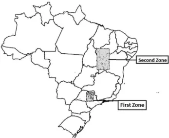
The homogeneous zones are identified according to the similarity of their rainfall probability distributions and delimited using the hierarchical cluster analysis obtaining 25 rainfall homogeneous zones in Brazil. Two homoge-neous zones were chosen. The first zone covers the states of São Paulo within a rectangle with latitude ranging from -23.0 to -20.5 and longitude of -49.5 and -47.5 with 103 weather stations. The second zone included 51 weather sta-tions located in the northeast of Brazil, within the rectangle defined with latitude ranging from -14.0 to -8.0 and longi-tude between -46.5 to -43.0. The first homogeneous zone is a climatic transition zone with average rainfall. In the sec-ond homogeneous area dominates the semi-arid tropical climate of low rainfall.
The spatio-temporal model for each set of data from each zone was adjusted using programs developed in R lan-guage (R Development Core Team, 2011) with the support of the Stem library (Spatio-temporal models in R) (Came-letti, 2009). In order to improve the estimates of the model parameters, the altitude of the stations was used as a cova-riate.
The spatio-temporal model used is discussed follow-ing Fassò and Cameletti (2009). Let Z (s,t) be a scalar spatio-temporal process observed at time t and geograph-ical location s. LetZt= {(s1,t), ...,Z(sn,t)} be a dataset at
time t for n geographic locationss1, ..., sn. Moreover, let
Yt = {Y1(t), ..., Yp (t)} be a vector of p dimension of a
not-observed temporal process at time t withp£n. The hi-erarchical three stage model fort= 1, ...,Tis defined as fol-lows:
Zt =Ut +rt
e (1)
Ut =Xt +KYt + t
r
r
b w (2)
Yt =GYt-1+ t
r
In Eq. (1), the erroretis introduced so thatUtis re-garded as a smoothed version of the spactio-temporal pro-cess Zt. In Eq. (2), the not-observed spatio-temporal processUtis defined as the sum of three components: theXt matrix of observed covariates for the time t for n locations, the latent spatio-temporal processYtand thewterror mo-del. Finally, the Eq. (3) is modeled as an autoregressive pro-cess where G is the matrix of transition and ht is the innovation error. The errorset,wtandhthave zero mean and are time-independent and independent from each other. Substituting Eq. (2) into Eq. (1) results in the following hi-erarchical two stages model:
Zt =Xt +KYt + t
r
r
b e (4)
Yt =GYt-1+ t
r
h (5)
Equations (4) and (5) are the state-space model equa-tions (Durbin and Koopman, 2001; Carvalhoet al., 2011; Chui and Chen, 2009). Eq. (4) is the equation of measure-ments and Eq. (5) is the equation of state. TheYttemporal process can be estimated using the Kalman filter or Kalman smoother.
In Eq. (4), the erroret = t + t
r r
w e is normally distrib-uted with zero mean and variance and covariance matrix
r r
r
Se =sw2G i- j i j= n
1
(s s ), ,... , (6)
wherer
Gis the spatial covariance function defined as
r
G ( )d q, q
d
h h
C h h
= + = > ì í î 1 0 0 if if
( ) (7)
and d s s e w = 2 2 (8)
In geostatistics, the errorse2 is the nugget effect for the spatial process (s,t) for a fixedt. The vector of para-meters to be estimated is { ,r , ,r , , log , ,}
r
b sw m se d q
2 2
GSn n = ,
whereb= regression matrix,sw2 = spatial variance,
G= tran-sition matrix of the autoregressive process,r
Sn = Kalman
filter variance covariance matrix, r
mn = Kalman filter means,se2= nugget effect, andq= spatial process.
Among the known approaches to perform parameter estimations, one can cite the maximum likelihood tech-niques involving the use of scoring techtech-niques or the New-ton-Raphson method for solving non-linear equations arising from the differentiation of the log likelihood func-tion. The likelihood methods usually have several undesir-able characteristics such as inversion of large Hessian matrices, the instability of the numerical maximization pro-cess and the resulting non-positive definite matrices (Fassò and Cameletti, 2009, 2010). To avoid these problems, the Stem library uses the EM algorithm (Shumway and Stoffer,
1982; Mclachlan and Krishnan, 1997), which is widely used for problems with missing values, as it is the case for Eqs. (4) and (5) where the component of missing values is given by the latent variableYt.
Since the EM algorithm does not use a Hessian matrix in the log-likelihood function, it does not provide standard errors for use with the estimated parameters, as the New-ton-Raphson algorithm does. Hence, the bootstrap method is used mainly for the estimation of EM to obtain an esti-mate of the standard errors.
Bootstrap methods are computationally intensive me-thods of statistical analysis that uses simulation to calculate standard errors and confidence intervals. These methods are applicable to any level of modeling, and thus can be used in both parametric and non- parametric analysis (Efron and Tibshirani, 2003).
To validate the values obtained using the spatio-tem-poral model, for the study zones, two dates were chosen, January 1, 2012 and May 1, 2012. For these fixed times, or-dinary kriging and cokriging geostatistical techniques (Yamamoto and Landim, 2013) were used with altitude as a covariate, to estimate missing values by cross-validation assuming that one of the sample elements, was not ob-served.
The first date corresponds to the rainy season in the first homogeneous zone of Brazil. In the second homoge-neous zone, this date is during the dry season. The second date, represents the dry season in the first homogeneous zone of the study area and the rainy season for the second homogeneous zone. According to these criteria, the best in-terpolation for each variable, is one that has the lowest value for the Mean Squared Error (MSE), that is, the ratio of the squared difference between the observed value and the estimated value divided by the number of observations. It is expected that by setting two distinct dates, the best per-formance of the estimates are obtained by the spatio-tem-poral model.
It is quite common in verification studies to use the statistic SS (Skill Score) to summarize the quality of the forecasting system. This score quantifies the relative varia-tion of the mean square error of the spatio-temporal model (MSEmod) with regard to the kriging and cokriging (MSEkrig
and MSEcockri). Positive values of SS indicate that the
model improved the predictions (Carvalho et al., 2011; Libonatiet al., 2008).
SS MSE MSE
MSE 1
krig mod
krig
= - ´100% (9)
SS MSE MSE
MSE 2
cokrig mod
cokrig
3. Results and Discussion
For 2012, 103 weather stations with complete data se-ries were selected in the first homogeneous zone and 51 weather stations for the second homogeneous zone (365 days of precipitation values). Figure 1 shows the spatial dis-tribution of rainfall observations used in this study by zone.
For the first and second homogeneous zones, random data samples of six weather stations were taken out and es-timates of the same values for the spatio-temporal pattern and geostatistical interpolation using values of neighboring points were obtained. Estimates of daily rainfall for January 1, 2012 and May 1, 2012 using the spatio-temporal model, kriging and cokriging methods are shown in Tables 1 and 2 respectively.
The statistics Skill Score (SS1 and SS2) (Eqs. (9)
-(10), respectively) are used to quantify, as a percentage, the
improvement that occurred in the estimation of daily rain-fall data for the two dates, using the spatio-temporal model in relation to the estimates obtained by kriging and cokriging. For the first date in the first zone, the estimate obtained by the spatio-temporal model was 24.41% better than the estimate obtained by kriging (SS1) and 17.77%
better than the estimate obtained by cokriging (SS2). For the
second date in the same zone, the spatio-temporal model was 32.12% and 26.16% better. The statistical skill score has been used in several studies with good results, as in Carvalhoet al.(2011) in Kalman filter and correction of the temperatures estimated by PRECIS model.
For the second zone, the estimates obtained by the spatio-temporal model were always better than the esti-mates obtained by kriging and cokriging. In all cases, the mean squared errors obtained by the model (MSEmod) were
considerably less than the mean squared errors obtained by kriging (MSEkrig) and cokriging (MSEcokrig).
In both zones the result obtained by the spatio-tem-poral model is always better indicating that neither the year nor the station influences the results. However, the results of the three methods for second zone are considerably lower compared to the first zone. Amisigo and Giesen (2005) also obtained better results by estimating gaps in daily riverflow series using spatio-temporal modelling. As well as, Francisconet al.(2008) when she modeled the inci-dence of citrus leprosis using spatio-temporal autologistic model and Ruiz-Cárdenas et al. (2009) using the same model to estimate better values when the temporal series is inflated with zeroes and missing values.
4. Conclusions
• The application of a spatio-temporal model produced
better estimates of daily precipitation values compared with results obtained by geostatistical kriging and cokriging models for the study period.
• The spatio-temporal model proved to be a versatile
tech-nique, adapting to different seasons, and should be con-sidered as an alternative to fill gaps in time series.
• The mean squared errors obtained by the model were
considerably less than the mean squared errors obtained by kriging and cokriging.
• For the two time periods studied, predictions using the
spatio-temporal model were more than 17% better for first zone and more than 26% better for second zone, compared to the forecasts obtained by geostatistical techniques.
Acknowledgments
The authors would like to thank the anonymous re-viewers for the considerable contribution.
Figura 1- Spatial distribution of rainfall observations for first zone and second zone.
Tabela 1- Mean Square Error for estimates of gaps obtained from the spatio-temporal model (MSEmod), kriging (MSEkrig) and cokriging (MSEcokrig) on January 1, 2012 – SS1and SS2are the Skill-Score statistics when comparing the model with kriging and cokriging, respectively.
Zone MSEmod MSEkrig SS1(%) MSEcokrig SS2(%) First 19.77 26.15 24.41 24.04 17.77 Second 4.60 5.44 18.51 5.62 18.20
Tabela 2- Mean Square Error for estimates of gaps obtained by the spatio-temporal model (MSEmod), kriging (MSEkrig) and cokriging (MSEcokrig) on May 1, 2012 - SS1and SS2are the Skill-Score statistics when comparing the model with kriging and cokriging, respectively.
References
AMISIGO, B.A.; GIESEN, N.C. van de. Using a spatio-temporal dynamic state-space model with the EM algorithm to patch gaps in daily riverflow series.Hydrology and Earth Sys-tem Sciences, v. 9, p. 209-224, 2005.
BAJAT, B.; PEJOVIC, M.; LUKOVIC, J.; MANOJLOVIC, P.; DUCIC, V.; MUSTAFIC, S. Mapping average annual pre-cipitation in Serbia (1961-1990) by using regression kriging.
Theoretical and Applied Climatology, v. 112, n. 1-2, p. 1-13, 2013.
CAMELETTI, M. Spatio-temporal models in R. 2009. Availabe in: http://cran.r-project.org/web/packages/Stem/index.html. Access in: Nov. 2014.
CARVALHO, J.R.P de; ASSAD, E.D.; PINTO, H.S. Kalman fil-ter and correction of the temperatures estimated by PRECIS model.Atmospheric Research, v. 102, n. 1-2, p. 218-226, 2011.
CHUI, C.K.; CHEN, G.Kalman filtering with real-time appli-cations. Berlin: Springer-Verlag Berlin Heidelberg, 2009.
229 p.
CRESSIE, N.; WIKLE, C. Space-time kalman filter. In: EL SHA-ARAWI, A.; PIEGORSCH, W. (Ed.). Encyclopedia of environmetrics. New York: Wiley, 2002. v. 4, p.
2045-2049.
DURBIN, J.; KOOPMAN, S. Time series analysis by state space methods. New York: Oxford University Press, 2001.
346 p.
EFRON, B.; TIBSHIRANI, R.J.An introduction to the boot-strap. London: Chapman and Hall, 2003. 436 p.
EMBRAPA INFORMÁTICA AGROPECUÁRIA.Agritempo -Sistema de Monitoramento Agrometeorológico.
Campi-nas, 2014. Available in: www.agritempo.gov.br/. Access in: Oct. 2014.
FASSÒ, A.; CAMELETTI, M.A. The EM algorithm in a distrib-uted computing environment for modelling environmental space-time data.Environmental Modelling & Software, v.
24, n. 9, p. 1027-1035, 2009.
FASSÒ, A.; CAMELETTI, M.A. A unified statistical approach for simulation, modeling, analysis and mapping of environ-mental data. Simulation:Transactions of the Society for
Modeling and Simulation International, v.86, n. 3, p. 139-154, 2010.
FOWLER, H.J.; BLENKINSOP, S.; TEBALDI, C. Linking cli-mate change modelling to impacts studies: recent advances in downscaling techniques for hydrological modelling.Int. J. Climatol., v. 27, n. 12, p. 1547-1578, 2007.
FRANCISCON, L.; RIBEIRO JUNIOR, P.J; KRAINSKI, E.T.; BASSANEZI, R.B.; CZERMAINSKI, A.B. C. Modelo autologístico espaço-temporal com aplicação à análise de padrões espaciais da leprose-dos-citros. Pesq. Agropec. Bras., v. 43, n. 12, p. 1677-1682, 2008.
GOODALL, C.; MARDIA, K.V. Challenges in multivariate spa-tio-temporal modeling. In:International Biometric Con-ference, 17, 1994, Ontario, Canada. Proceedings. [Ontario]:
McMaster University Press, 1994. p. 1-17.
HASLETT, J. Space-time modelling in meteorology - a review.
Bulletin Statistical Institute, v. 51, p. 229-246, 1989.
HAWORTH, J.; CHENG, T. Non-parametric regression for space-time forecasting under missing data.Computers En-vironment band Urban Systems, v. 36, p. 538-550, 2012. KELLER FILHO, T.; ASSAD, E.D.; LIMA, P.R.S.R. Regiões pluviometricamente homogêneas no Brasil.Pesq. Agropec. Bras., v. 40, n. 4, p. 311-322, 2005.
LASINIO, G.J.; SAHU, S.K.; MARDIA, K.V. Modeling rainfall data using a Bayesian Kriged-Kalman model. In: UPADHYAY, S. K.; SINGH, UMESH; Dey, Dipak K. (Ed.).Bayesian statistics and its applications. Tunbridge
Wells, UK: Anshan, 2007. p. 61-86.
LAU, M.S.Y.; MARION, G.; STREFTARIS, G.; GIBSON, G.J. New model diagnostics for spatio-temporal systems in epi-demiology and ecology. J. R. Soc. Interface, n. 11:20131093 http://dx.doi.org/10.1098/rsif.2013.1093. LI, Y.Y.; PARKER, L.E. A spatial-temporal imputation
tech-nique for classification with missing data in a wireless sen-sor network.IEEE International Conference On Intelli-gent Robots And Systems, 2008, Nice, France.
Proceedings [Nice].
LIBONATI, R.; TRIGO, I., DACAMARA, C.C. Corrections of 2 m-temperature forecasts using Kalman filtering technique.
Atmospheric Research, v. 87, n. 2, p. 183-197, 2008.
LO PRESTI, R.; BARCA, E.; PASSARELLA, G.A. methodology for treating missing data applied to daily rainfall data in the Candelaro River Basin (Italy).Environmental Monitoring and Assessment, v. 160, n. 1-4, p. 1-22, 2010.
LOU, Q.; OBRADOVIC, Z. Modeling multivariate spatio-tem-poral remote sensing data with large gaps. International Joint Conference On Artificial Intelligence 22, 2011, Bar-celona, Spain. Proceedings [Barcelona].
MCLACHLAN, G.J.; KRISHNAN, T.The Em algorithm and extensions.New York: Wiley, 1997. 400 p.
MARDIA, K.V.; GOODALL, C.; REDFERN, E.J.; ALONSO, F.J. The Kriged Kalman filter (with discussion).Test, v. 7, p. 217-252, 1998.
PEREIRA, A.R.; ANGELOCCI, L.R.; SENTELHAS, P.C. Agro-meteorologia:fundamentos e aplicações práticas. Guaíba: Livraria e Editora Agropecuária, 2002. 478 p.
R DEVELOPMENT CORE TEAM. R: A language and environ-ment for statistical computing. Vienna: TheR Foundation for Statistical Computing, 2011. Available in:
http://www.gbif.org/resource/81287. Access in: Jan. 2015. ROUHANI, S.; MYERS, D.E. Problems in space-time kriging of
geohydrological data.Mathematical Geology, v. 22, n. 5,
p. 611-623, 1990.
RUIZ-CÁRDENAS, R.; ASSUNÇÃO, R.M., DEMÉTRIO, C.G.B. Spatio-Temporal modelling of coffee berry borer in-festation patterns accounting for inflation of zeroes and missing values.Sci. Agric., v. 66, n. 1, p. 100-109, 2009. SHUMWAY, R.H.; STOFFER, D.S. An approach to time series
smoothing and forecasting using the EM algorithm.Journal of Time Series Analysis, v. 3, n. 4, p. 253-264, 1982. SOARES, F.S.; FRANCISCO, C.N.; SENNA, M.C.A.
Distri-buição espaço-temporal da precipitação na Região Hidro-gráfica da Baía da Ilha Grande - RJ.Revista Brasileira de Meteorologia, v. 29, n. 1, p. 125-138, 2014.
LÓPEZ-MORENO, J.I.; GARCÍA-VERA, M.A.; STEPANEK, P. A complete daily precipitation database for northeast Spain: reconstruction, quality control, and homogeneity. Int. J. Climatol., v. 30, p. 1146-1163, 2010.
YAMAMOTO, J.K.; LANDIM, P.M.B.Geoestatística:conceito
e aplicações. São Paulo: Oficina de Textos, 2013. 215 p.
YOUNG, K.C. A three-way model for interpolating for monthly precipitation values.Mon. Weather Rev., v. 120, p. 2561-2569, 1992.