KNOWLEDGE DISCOVERY FROM TRAJECTORIES

(1)

KNOWLEDGE DISCOVERY FROM TRAJECTORIES

(2)

K

NOWLEDGE

D

ISCOVERY FROM

T

RAJECTORIES

Dissertation supervised by Professor Fernando Bação, Ph.D

Dissertation co-supervised by Professor Laura Diaz, Ph.D Professor Miguel Neto, Ph.D

(3)

ACKNOWLEDGEMENTS

I would like to thank Professor Bação for leading me into this amazing world of data mining. Also many thanks to Professor Painho, the best director I have ever seen, and Professors Michael Gould, Laura Diaz, Miguel Neto for their support, advice and feedback.

Additionally, I will say thanks to Professors Laube, Gennady, Bogorny and Cooley for helping me looking for appropriate data set. Special thank you should goes to Professor Gennady for helping me get access to his software. I have to say his software is amazing. Also thank Robert for helping me to solve all problems related with Geo-SOM. Other thanks are to all the staffs working in ISEGI, your warmth and hospitality make me feel like at home.

(4)

K

NOWLEDGE

D

ISCOVERY FROM

T

RAJECTORIES

ABSTRACT

(5)

KEYWORDS

Data mining Elk

Knowledge discovery Spatio-temporal patterns Starkey Project

Taxonomy

(6)

ACRONYMS

BMU – Best Matching Units

CB-SMOT – Clustering-based Stops And Moves of Trajectories

DBSCAN – Density-Based Spatial Clustering of Applications with Noise

FSP – Frequent Sequential Pattern

Geo-SOM – Geo-Self-Organizing Map

GI – Geographic Information

GKD – Geographic Knowledge Discovery

GMT – Greenwich Mean Time

GPS – Global Positioning Systems

GSM – Global System for Mobile communications

KDD – Knowledge Discovery from Databases

LBS – Location Based Services

LCSS – Least Common Sub-Sequence

OPTICS – Ordering Points To Identify the Clustering Structure

RFID – Radio Frequency Identification Tags

RoIs – Regions of Interest

SMOT – Stops and Moves of Trajectories

SOM – Self-Organizing Maps

STARs – Spatio-temporal Association Rules

UTM – Universal Transverse Mercator

(7)

INDEX OF TABLES

Table 1: Classification of trajectory data based on moving objects ... 14

Table 2: Classification of trajectory data based on format of locations ... 16

Table 3: Class and Cluster patterns ... 21

Table 4: Potentially helpful environmental variables ... 55

(10)

INDEX OF FIGURES

Figure 1: Some common movement patterns ... 5

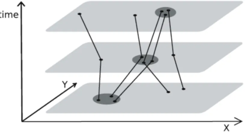
Figure 2: Space-time diagram showing residents in their daily lives ... 18

Figure 3: Groups of trajectories ... 20

Figure 4: Example of moving clusters ... 21

Figure 5: The geospatial lifelines of four MPOs and analysis in REMO ... 29

Figure 6: The constraints of the patterns track, flock and leadership ... 31

Figure 7: Geometric detection of convergence. ... 32

Figure 8: The location of Starkey Project... 36

Figure 9: Two elk tracks in May, 1996. ... 37

Figure 10: Parallel box plot of estimated elk speeds by hour of the day ... 38

Figure 11: Kernel density estimates of elks at noon during spring ... 39

Figure 12: Temporal distribution of samples from 2 May to 15 August, 1996 ... 41

Figure 13: Samples' distribution among elks ... 42

Figure 14: Rediscretization of original unevenly sampled data set ... 43

Figure 15: Four different perspectives to derive the movement azimuth. ... 44

Figure 16: Point and line density of elk distribution ... 53

Figure 17: Elk distribution at different period of a day ... 54

Figure 18: Geo-SOM architecture ... 57

Figure 19: Results after applying Geo-SOM on elks’ locations during daytime ... 58

Figure 20: Results after applying Geo-SOM on elks’ locations during midnight ... 59

Figure 21: RoIs produced by Minimum Convex Hull ... 60

Figure 22: Histogram of trajectory durations after partitioning ... 60

Figure 23: Histogram of the least 20% of trajectory durations after partitioning ... 61

Figure 24: Two clusters generated after first clustering ... 63

Figure 25: Three clusters generated after second clustering ... 63

Figure 26: Three clusters generated after third clustering. ... 64

(11)

1 Introduction

Trajectories are ubiquitous in the real world. As long as an object is moving, no matter it is as huge as a planet or as tiny as an electron, no matter it is a cannonball or a home letter, trajectory is being produced like a long tail. The only difference among them is some movements follow the rule set by Sir Isaac Newton, like guided missile and satellite, while others are under the control of God: God knows where I will go after finishing this thesis. This research is focused on the “unpredictable” trajectories and will start with introducing in the key terms in this context.

1.1 Trajectories

Common sense tells us trajectory is the track of water mark behind a sprinkler vehicle rambling on the street. But a more rigorous definition for scientific research is needed.

In database community, trajectories, which usually stored in moving objects databases (sometimes called trajectory databases in the literature), describe complete histories of movement. A definition giving trajectories semantic meaning was proposed by (Spaccapietra et al. 2008).

“A trajectory is the user defined record of the evolution of the position (perceived as a point) of

an object that is moving in space during a given time interval in order to achieve a given goal. Trajectory:

[t _begin, t _end] → space.”

In Geographical Information (GI) science community, people often use the term Geospatial lifeline, inspired by time-geography (Hägerstraand 1970; Hägerstrand 1976; Parkes et al. 1980), as a representation of an individual’s movement pattern in geographic space.

“A geospatial lifeline is … the continuous set of positions occupied by an object in geographic

space over some time period. Geospatial lifeline data consist of discrete space-time observations of a

geospatial lifeline, describing an individual’s location in geographic space at regular or irregular temporal

intervals.” (Mark et al. 1998).

(12)

animals bearing a transmitter, parcels tagged with RFIDs and hurricane tracking data from meteorological satellites.

The basic element of trajectories is a space-time observation consisting of a triple (ID, Location, Time), where ID, sometimes optional, is a unique identifier of the individual used throughout all recordings of that individual’s movements, Location is a spatial descriptor (such as a coordinate pair, a polygon, a street address, or some other locative expression), and Time is the time stamp when the individual was at that particular location (such as a clock time in minutes or event time in years) (Spaccapietra et al. 2008).

In addition, this thesis use the term trajectory instead of spatio-temporal data is to exclude another class of spatio-temporal data set recording spatio-temporal events, such as the records of crime, traffic accident. These events share the same (ID, Location, Time) structure and also applicable to some knowledge discover techniques used in this thesis. But it is beyond the scope of this study.

1.2 Knowledge Discovery

1.2.1 Traditional Knowledge Discovery

Knowledge discovery is often used as a part in the acronym KDD (Knowledge Discovery from Databases), in this case, we are applying it to trajectory databases. KDD is the higher level process of obtaining facts through data mining and distilling this information into knowledge or ideas about the mini-world described by the data. This generally requires a human-level intelligence to guide the process and interpret the results based on pre-existing knowledge (Miller et al. 2001). The KDD process does not seek any arbitrary pattern from a database; rather, data mining seeks only those that are interesting. These patterns are valid (a generalizable pattern, not simply a data anomaly), novel (unexpected), useful (relevant) and understandable (can be interpreted and distilled into knowledge) (Fayyad et al. 1996). The KDD process typically involves the following major steps grouped into larger activity categories (Fayyad et al. 1996; Miller et al. 2001; Qi et al. 2003), which we will also be followed in this study.

1. Background

(13)

2. Data pre-processing

2.1 Data selection, or determining a subset of the records or variables in the database for focusing the search for interesting patterns.

2.2 Data cleaning, including removal of noise and outliers.

2.3 Data reduction, including transformations, projections and aggregations to find useful representations for the data.

3. Data mining

3.1 Choosing the data mining task. This involves selecting the generic type of pattern sought through data mining; this is the language for expressing facts in the database. Generic pattern types include classes, associations, rules, clusters, outliers and trends.

3.2 Choosing the data mining technique for discovering patterns of the generic type selected in the previous step. Since data mining algorithms are often heuristics (due to scalability requirements), there are typically several techniques available for a given pattern type, with different techniques concentrating on different properties or possible relationships among the data objects.

3.3 Data mining: applying the data mining technique to search for interesting patterns.

4. Knowledge construction

4.1 Interpreting the mined patterns, often through visualization.

4.2 Consolidating the discovered knowledge, either by incorporating the knowledge into a computational system (such as a knowledge-based database) or through documenting and reporting the knowledge to interested parties.

1.2.2 Geographical Knowledge Discovery

Geographic knowledge discovery (GKD) is the process of extracting information and knowledge from massive geo-referenced databases. The nature of geographic entities, relationships and data means that standard KDD techniques are not sufficient (Shekhar et al. 2003).

(14)

defined in highly general terms, including distance, direction and/or topology. Spatial heterogeneity or the non-stationarity of the process with respect to location is often evident since many geographic processes are local.

Including time introduces additional complexity to the GKD process. A simple strategy that treats time as an additional spatial dimension is not sufficient. Time has different semantics than space: time is directional, has unique scaling and granularity properties, and can be cyclical and even branching with parallel local time streams (Roddick et al. 2001).

1.3 Spatio-temporal patterns

As the knowledge discovered from trajectories, the Spatio-temporal patterns should also be valid, novel, useful and understandable. Additionally, due to the innate semantics of spatial and temporal attributes, the number of possible patterns produced by this combination can hardly be exhausted. Roddick and Lees (2001) even argued that the potential complexity of spatio-temporal patterns may require meta-mining techniques that search for higher-level patterns among the large number of patterns generated from spatio-temporal mining. In this section, some common patterns that may be discovered from trajectories are listed as examples, later in this thesis, the patterns documented by researches will be further discussed along with the knowledge discovery techniques, also, a preliminary taxonomy will be proposed.

A class of spatio-temporal patterns is named movement patterns, which in trajectory data, refer to salient events and episodes expressed by a set of entities. In the case of moving animals, movement patterns can be viewed as the spatio-temporal expression of behaviors, as for example in flocking sheep or birds assembling for the seasonal migration. In a transportation context, a movement pattern could be a traffic jam (Gudmundsson et al. 2008) .

(15)

Figure 1: Some common movement patterns (Gudmundsson et al. 2008)

Another class of spatio-temporal patterns is spatio-temporal association rules (STARs). Just like diaper and beer often appear together in the shopping basket, s convenient analogy can be two places in one trip of a moving entity. In practice, this rule is often mined after transforming the trajectory into a series of semantic meaningful places or a series of regions passing by. However, besides using places, other features such as a U-turn in a trip and spatio-temporal attributes of the trajectory can also be used to derive association rules. In addition, a temporal annotation can be attached to the rules, thus the rule can be an object (satisfying some conditions) will show up at place B one hour after going to place A.

1.4 Motivation

(16)

1.4.1 Proliferating data

The availability of trajectory data is the initial driving force and perquisite of related research. Thanks to technical progress on satellite, sensor, RFID (Radio Frequency Identification Tags), video and wireless technologies, especially as mobile devices proliferate and networks become more location aware, large scale capture of the evolving position of individual mobile objects has become technically and economically feasible. The corresponding growth in spatio-temporal data will demand analysis techniques to mine patterns that take into account the semantics of such data.

In addition, for high resolution tracking data, the most distinctive feature is that they allow the track of individuals along an actual movement path, leaving little need for interpretation between sparse observation points. Thus, at almost every instant along the lifeline we can robustly determine the individual’s current movement properties, such as speed, acceleration, motion azimuth, path sinuosity, as well as generate even more complex motion properties (Laube et al. 2007).

1.4.2 Potential applications

The availability of trajectory data set opens new perspectives for a large number of applications (from e.g. transportation and logistics to ecology and anthropology) built on the knowledge of movements of objects (Spaccapietra et al. 2008). Some key application fields have been identified by Gudmundssonet al. (2008) as follows:

1.4.2.1 Animal Behavior

(17)

animals. It is possible to investigate social interactions, ultimately revealing the social structure within a group of animals. A major focus lies on the investigation of leading and following behavior in socially interacting animals, such as in a flock of sheep or a pack of wolves (Dumont et al. 2005). Advanced path analysis is considered to be a crucial obligation for the interpretation of behavioral experiments conducted with genetically modified animals, for example for water maze experiments with mice exploring spatial learning (Wolfer et al. 2001). Similar analysis is also of increasing interest in agricultural science, contributing to the development, for example, of optimal grazing strategies for cattle with respect to livestock management (Ganskopp 2001). On a larger scale, animal movement data reflects very well the seasonal or permanent migration behavior. In the animation industry, software agents implement movement patterns in order to realistically mimic the behavior of animal groups. Most prominent is the flocking model implemented in NetLogo which mimics the flocking of birds (Wilensky 1998).

1.4.2.2 Human Movement

(18)

1.4.2.3 Traffic Management

Movement patterns are used for traffic management in order to detect undesirable or even dangerous constellations of moving entities, such as traffic jams or airplane course conflicts. Traffic management applications may require basic Moving Object Database queries, but also more sophisticated movement patterns involving not just location but also speed, movement direction and other activity parameters.

1.4.2.4 Surveillance and Security Surveillance

Research involving video surveillance (Ng 2001; Porikli 2004; Shim et al. 2003) might have access to more detailed data sets capturing the movement of people, e.g. coordinates from mobile phones or credit card usage, video surveillance camera footage or maybe even GPS data. Apart from analyzing the movement data of a suspect to help prevent further crime, it is an important task to analyze the entire data set to identify suspicious behavior in the first place. This leads to define `normal behavior' and then search the data for any outliers, i.e. entities that do not show normal behavior. Some specific activities and the corresponding movement patterns of the involved moving entities express predefined signatures that can be automatically detected in spatio-temporal or footage data. One example is that fishing boats in the sea around Australia have to report their location in fixed intervals. This is important for the coast guards in case of an emergency, but the data can also be used to identify illegal fishing in certain areas. Another example is that a car thief is expected to move in a very characteristic and hence detectable way across a surveyed car park. Movement patterns have furthermore attracted huge interests in the field of spatial intelligence and disaster management. Batty et al. (2003) investigated local pedestrian movement in the context of disaster evacuation where movement patterns such as congestion or crowding are key safety issues.

1.4.2.5 Military and Battlefield

(19)

range queries like “Report all friendly tanks that are currently in region S.” A more complex movement pattern in a digital battlefield context would be the identification of the convergence area where the enemy is currently concentrating his troops.

1.4.2.6 Sports Scene Analysis

Research involving sports scene analysis (Moore et al. 2003) are further examples exhibiting deep interests in individual trajectories. Advancements in many different areas in technology are influencing professional sports. For example, some of the major tennis tournaments provide three-dimensional reconstructions of every single point played, tracking the players and the balls. It is furthermore known that, e.g. football coaches routinely analyze match video archives to learn about an opponent’s behaviors and strategies. Making use of tracking technology, the movement of the players and the ball can be described by 23 trajectories over the length of the match. Researchers were able to develop a model that is based on the interactions between the players and the ball. This model can be used to quantitatively express the performance of players, and more general, it might lead to an improved overall strategy. Finally, real-time tracking systems are developed that keep track of both players and the ball in order to assist the referee with the detection of the well-defined but nevertheless hard to perceive offside pattern.

1.4.2.7 Movement in Abstract Spaces

(20)

1.4.3 Challenges facing

While there is a growing commitment of resources to the large-scale recording of paths, the analysis commonly conducted with trajectory data remains fairly limited in scope and sophistication (Wolfer et al. 2001). In disciplines outside of geography do not commonly use geospatial methods or theory this may be due to a lack of awareness and understanding of the power of spatial analysis and GI system, and within geography GI science’s fetish for the static may be a factor (Raper 2002).

The challenges GI science is facing in developing analytical tools are well documented (Andrienko et al. 2006; Miller et al. 2001) and listed as follows.

a) The spatial relations, both metric (such as distance) and non-metric (such as topology, direction, shape, etc.) and the temporal relations (such as before and after) are information bearing and therefore need to be considered in the data mining methods.

b) Some spatial and temporal relations are implicitly defined, that is, they are not explicitly encoded in a database. These relations must be extracted from the data and there is a trade-off between precomputing them before the actual mining process starts (eager approach) and computing them on-the-fly when they are actually needed (lazy approach). Moreover, despite much formalization of space and time relations available in spatio-temporal reasoning, the extraction of spatial/temporal relations implicitly defined in the data introduces some degree of fuzziness that may have a large impact on the results of the data mining process.

c) Working at the level of stored data, that is, geometric representations (points, lines and regions) for spatial data or time stamps for temporal data, is often undesirable. For instance, urban planning researchers are interested in possible relations between two roads, which either cross each other, or run parallel, or can be confluent, independently of the fact that the two roads are represented by one or more tuples of a relational table. Therefore, complex transformations are required to describe the units of analysis at higher conceptual levels, where human-interpretable properties and relations are expressed.

(21)

e) Many rules of qualitative reasoning on spatial and temporal data (e.g., transitive properties for temporal relations after and before), as well as spatio-temporal ontologies, provide a valuable source of domain independent knowledge that should be taken into account when generating patterns. How to express these rules and how to integrate spatio-temporal reasoning mechanisms in data mining systems are still open problems.

f) Irregularity and Asynchronism: Many types of numerical temporal data are not uniformly and regularly sampled. Also in distributed computing environments like sensor networks, data from different sources might not to be perfectly aligned and hence synchronous methods are inapplicable before rediscretization.

g) Huge volume: The stream of data can be huge for a long, continuous observation period. Many types of measurements can be obtained from a large number of data sources. This requires designing scalable solutions in analyzing a large volume of temporal data, in terms of both the large number of data points and the large number of types of measurements.

h) Exploratory (spatial) data analysis (Anselin 1998) has been identifies as a good way to explore not only spatial but also spatio-temporal data. However, it has also been acknowledged that visual inspection reaches its limits if numbers of moving point objects and lengths of lifelines increase(Kwan 2000).

i) Additional research issues related to spatio-temporal data mining concern data structures used to represent and efficiently index spatio-temporal data.

1.5 Research context and objectives

(22)

Until now the studies in this area are insufficient in many aspects. From the very beginning, the authors often neglect the category of target data sets their methods can be applied to. For example, some methods may be applicable to a single long trajectory, while some methods are only for multiple trajectories. The semantic meaning of discovered patterns also varies correspondingly. Let alone the impact of uncertainty and granularity, which is seldom mentioned in most studies. Secondly, most researches discuss some simple classes of patterns and focuses mainly on algorithmic aspects. These algorithms often neglect the numerous possibilities produced by the special form of trajectories in different semantic context, like the definition of similarity of trajectories. Lastly, the great power of spatial analysis and visualization provided by GI systems is often neglected by researchers from data mining community.

Thus this thesis tentatively classifies all kinds of trajectory data available until now (input) and spatial-temporal patterns (output) respectively. The algorithms (methodology) appeared on papers are put in their applicable range to bridge the data and pattern. Then a real data set is put into this framework to explore the possible patterns and applicable methodology. Standard knowledge discovery procedure is followed along with an emphasis on preprocessing and visualization in GI system. More specifically, the objective of this study will be achieved by fulfilling the four tasks:

¾ T1: Classification of trajectory data sets

¾ T2: Classification of spatio-temporal patterns corresponding to different trajectory data

¾ T3: Bridge the data sets and patterns with methodologies proposed by previous researchers and find out the blanks that should be filled

¾ T4: Put a real data set into this framework to explore possible patterns.

1.6 Overview of document

(23)

Due to the particularity aspects (e.g. there are very few studies systematically discuss patterns in trajectories) of this research, chapter 2 will not be a traditional literature review, instead, it is a theoretical framework built on related researches. So the details of algorithm are mostly only referred to corresponding papers to avoid diluting the main purpose of this study. As a result, some methods and algorithms used later in the following case study are introduced where they will be applied.

A real data set will be introduced in chapter 3 along with some background knowledge about the data set, and the preprocessing and exploratory analysis will be applied to this data set.

In chapter 4, frequently visited locations, which referred as Regions of Interest (RoIs) are derived from the Starkey data set. Then, after partitioning the trajectories using these RoIs, the trajectories are further clustered to find corridors among these RoIs.

(24)

2 Theoretical framework

As illustrated in previous chapter, the theoretical framework is comprised of three parts: trajectories, patterns and methodologies, which will be explored in the following three sections respectively.

2.1 Trajectories

The basic element of trajectories is a space-time observation consisting of a triple (ID, Location, Time). The classification of trajectories then can also be from three aspects: ID, Location, and Time.

2.1.1 ID

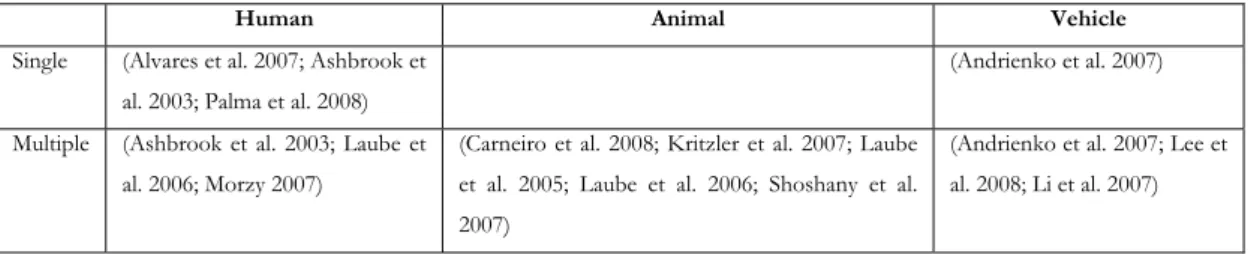
ID, the unique identification of location-aware devices bearer, is optional in the trajectory triple if only one moving object is studied. More often case is several or tens of objects are studied, which can produce more complex also more interesting patterns. Additionally, the typical bearers are mainly from three categories: human, animal and vehicle. Others like movement of hurricane landfall (Lee et al. 2007) rarely appears are not classified here. As an incomplete conclusion, table 1 shows a matrix of combination of these two factors and lists a few studies, not exhaustively, on each class of trajectories. No study on single trajectory of animal can be found, and there maybe two reasons explaining this. First, biologists are generally more interested in social behavior and spatial distribution, secondly, patterns shown in many animals as a group, like the Alzheimer-like pathology in laboratory mice (Kritzler et al. 2007), are more persuasive.

Human Animal Vehicle

Single (Alvares et al. 2007; Ashbrook et

al. 2003; Palma et al. 2008)

(Andrienko et al. 2007)

Multiple (Ashbrook et al. 2003; Laube et

al. 2006; Morzy 2007)

(Carneiro et al. 2008; Kritzler et al. 2007; Laube

et al. 2005; Laube et al. 2006; Shoshany et al.

2007)

(Andrienko et al. 2007; Lee et

al. 2008; Li et al. 2007)

Table 1: Classification of trajectory data based on moving objects

2.1.2 Location

(25)

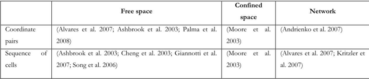
time, since in some sense, everything is moving in a confined space. The difference between then can be determined by the influence of border on movements. The football field is often too small for the 22 players while the ocean and sky is generally big enough for ships and birds. For the same reason, the movement of animal in pasture can be regarded as in free space if the range is big enough. Additionally, in some cases, due to the limitation of tracking technology, movement in free space can be tracked at only a few key places, which comprises a network instead (Kritzler et al. 2007).

Secondly, the locations can be of several formats. Most typical format of location is coordinates logged by GPS devices, which is a pair of latitude and longitude in WGS84 reference system. Another extensively studied format is that of data collected by mobile network using GSM (Global System for Mobile communications), which can only locate the mobile phone holder to a cell ranging several kilometers. Thus the data recorded is only sequences of different cells. The coordinate’s pairs can be rediscretized into sequences of cells, actually researchers did in many cases, by dividing the space into grids or only extract important places along the trajectories. A tradeoff between accuracy and mining efficiency is the reason behind the transformation.

A special case is the movement in abstract information space (Laube et al. 2006), where the coordinates can be arbitrary attributes instead of the latitude and longitude we often use, as a result, the border is proprietary to the attributes used.

An inevitable issue related to the location is uncertainty, which is an inherent characteristic of spatiotemporal data (Nanni et al. 2008). It arises due to physical and technical limitations during data collection and storage. Uncertainty of location varies with the applied technology between a few meters (GPS) and kilometers (GSM). In addition, the sampling rate possesses a great influence on accuracy. The faster an object move, to sustain a given level of spatial uncertainty, the more often must an object’s location be reported. Background knowledge as well as certain assumptions about movement behavior helps to reduce the uncertainty in data. For example, when tracking a vehicle, we can safely assume that all movements are restricted to the street network. Cars are unlikely to move through buildings.

(26)

P2 at times t1 and t2 and a maximum speed, an object’s position at each moment in time t ∈[t1,t2] is restricted to some area (Pfoser et al. 1999). If no further information is given, a uniform distribution of the objects within this area can be assumed.

Table 2, similar to table 1, shows the classification along with some studies. Some studies appear both as coordinate pairs and sequence of cells because there are rediscretization as mentioned above.

Free space Confined

space Network

Coordinate

pairs

(Alvares et al. 2007; Ashbrook et al. 2003; Palma et al.

2008)

(Moore et al.

2003)

(Andrienko et al. 2007)

Sequence of

cells

(Ashbrook et al. 2003; Cheng et al. 2003; Giannotti et al.

2007; Song et al. 2006)

(Moore et al.

2003)

(Alvares et al. 2007; Kritzler et

al. 2007)

Table 2: Classification of trajectory data based on format of locations

2.1.3 Time

Time is another special dimension besides location, which can be regarded as ratio, ordinal or cyclic variable in subsequent knowledge discovery process. Here in the classification of trajectory data, only temporal granularity need to be considered. The sampling interval can vary from seconds(Andrienko et al. 2007), hours(Rowland et al. 1997) to days (Carneiro et al. 2008). Also many types of numerical temporal data are not uniformly and regularly sampled. In distributed computing environments like sensor networks, data from different sources might not to be perfectly aligned and hence synchronous methods are inapplicable before rediscretization.

For high resolution tracking data, the most distinctive feature is that they allow the track of individuals along an actual movement path, leaving little need for interpretation between sparse observation points. Thus, at almost every instant along the lifeline we can robustly determine the individual’s current movement properties, such as speed, acceleration, motion azimuth, path sinuosity, as well as generate even more complex motion properties(Laube et al. 2007).

(27)

2.2 Spatio-temporal Patterns

The spatio-temporal patterns appeared on previous literatures are quite a lot. In this study, we are trying to apply a new taxonomy on these patterns. Our classification extends traditional methods, which are according to data mining techniques, by further classification considering output target and semantic meaning of space and time.

After applying the traditional classification method, i.e. considering the data mining techniques. The patterns are then classified as to the target these patterns are applied to. The target can be ID (a terrorist whose trajectory is unmoral or a bunch of people sharing some interest), or location (a frequently visited area or where traffic congestions often happen), or time (the time when football players slow down or birds start migration). It can also be some spatio-temporal phenomena, for example, the gridlock characterized by large amount of cars moving at low speed.

In the last step, these patterns are further classified according to their semantic meaning of space and time, i.e. the implicit spatial and temporal relations considered. For example, in periodical patterns, the time is regarded as cyclic, while other patterns often treat time as linear.

2.2.1 Classes, Clusters and Outliers

Clusters and classes are basically the same in the sense of similarity between trajectories. In practice, clustering is more often used since predefine the classes is often difficult. In addition, after defining these classes or extracting all the clusters, the leftover trajectories can be regarded as outlier.

2.2.1.1 ID

(28)

(29)

Just as the example in figure 2, the women’s daily movement can be classified into the six categories listed above. As we can see, the definition of these classes is far from exhausting the complexity of spatio-temporal classes. Let’s take the class “trajectories from home to kindergarten” as an example. This class can be extended from both spatial and temporal dimension.

At spatial dimension, there are two controlling points in the original definition, while the number of controlling points can be from 1 to positive indefinite. In the case of 1, a class can be defined as “trajectories leaving home”. In the case of more than 2, a class can be “trajectories from home to kindergarten passing by a shopping mall. By continuing adding control points, the definition is keeping narrowing down until trajectories whose shape is exactly the same are considered. In practice, it’s impossible to use indefinite number of controlling points, thus how to select controlling points, and how the points are distributed along the trajectories are all interesting topic to be discussed.

An implicit assumption above is that similarity of trajectories are based on the distance between controlling points, no matter the distance is metric (like Euclidean) or non-metric (like travelling time). A special but very useful variation is using semantics meaning of these control points instead of physical meaning. In this way, all trajectories in figure 3 are from their home to office, thus all will be classified together. However, until now, there is no exploration in this field due to the difficulty in semantics.

Since coordinates are innate interval attribute, the spatial translation and rotation can be applied if we only want to find cluster of trajectories of similar shape. For example, the trajectories of race cars can be clustered, and then players’ performance at different shape curves can be compared. This extension often applies when massive controlling points are used. Also, to avoid the influence of noise, i.e. some controlling points may highly deviate from the right track due to data collecting errors, the extraordinary distance between controlling points can be discarded using voting strategy or probabilistic modeling technique(Gaffney et al. 1999). Certainly, spatial distortion is mathematically feasible; nevertheless, no real life application is conceived.

(30)

spatio-temporal. As a result, in figure 3, the trajectories will be classified into three classes if more than 2 controlling points are considered, even though all trajectories from group 1, 2 and 3 are following the same route; i.e. only trajectories sharing the same route at the same time are regarded as in the same class. When time is treated at interval scale, i.e. the temporal translation is allowed, trajectories following the same route, but the time arriving at each controlling point differs at a given value. For example, group3 and group2, which are parallel in the spatio-temporal space, in figure 3 will be put into the same class. When time is treated as ordinal, i.e. only the sequence of locations is considered. The trajectories in group 1, 2 and 3 will all be recognized in the same class since the same route is followed. A special feature of time is it can be cyclic, like the yearly migration of birds and daily movement of human and vehicles. In this case, the time is ratio (can also be interval or ordinal) but temporal translation at given intervals is allowed. These intervals are often (1day, 2 days, 3 days …) or (1year, 2 years, 3 years …).

Figure 3: Groups of trajectories, edited from (Nanni et al. 2008)

A special extension of clustering is at ID dimension. This extension leads to a special pattern named moving clusters. As a nominal variable, ID is downgraded into a constant in the patterns in previous analysis. In figure 4, the notable cluster still exists at the three snapshots, but the members of this cluster keep changing. At last, only one

group 3 group 3

Home

Office Office

Home T8

T9

T1

T2

T3

T4 T5

T6

T7

(31)

object from the first snapshot stays in this cluster after two periods. Identifying these interesting clusters and studying their temporal evolving is of interest to many biologists.

Figure 4: Example of moving clusters (Nanni et al. 2008)

As a conclusion, the classification results from different class (cluster) patterns are listed in table 3 using the example trajectories in figure 3. The ordinal time is not applicable when only one controlling point is considered. The periodical patterns, corresponding to cyclic time cannot be found in this figure due to the difficulty in visualization. Which kind of spatial and temporal extension should be used to define classes and clusters at completely up to the knowledge we want to discover, for example, if we want to find all the (sub-)trajectories of somebody going home from office after finishing work, a two controlling points ratio plus cyclic extension is proper, because he may go home from office in the morning or at noon to fetch something forgotten bringing to office, which is not what we want.

Ratio Interval Ordinal Cyclic

One physical controlling points(take the

starting position of T1)

(T0, T1, T2, T3, T4,

T5); (T6, T7); (T8);

(T9)

(T0, T1, T2, T3, T4,

T5, T6, T7) ; (T8);

(T9)

N/A

periodical

patterns Two physical controlling points (starting

and finishing points)

(T0, T1, T2, T3, T4,

T5); (T6, T7) ; (T8);

(T9)

(T0, T1, T2, T3, T4,

T5, T6, T7) ; (T8);

(T9)

(T0, T1, T2, T3, T4,

T5, T6, T7) ; (T8);

(T9)

Several to massive physical controlling

points

(T0); (T1, T2, T3);

(T4, T5); (T6, T7) ;

(T8); (T9)

(T0); (T1, T2, T3);

(T4, T5, T6, T7);

(T8); (T9)

(T0); (T1, T2, T3,

T4, T5, T6, T7);

(T8); (T9)

Semantic controlling points (in this case,

only two points, home and office, have

semantic meaning)

(T0, T1, T2, T3, T4,

T5, T6, T7, T8, T9)

(T0, T1, T2, T3, T4,

T5, T6, T7, T8, T9)

(T0, T1, T2, T3, T4,

T5, T6, T7, T8, T9)

(32)

2.2.1.2 Location and time

The classes and clusters for location can be applied in two cases. The first one is using the result from previous section, i.e. a class or cluster of trajectories. Then the space and location occupied by these trajectories will be derived. For example, if trajectories between two semantically meaningful locations are identified as a cluster or class, their spatial projection will show the routes often used, which can be a corridor between animal habitats.

This also the case how classes and clusters are projected to time dimension and the time interval of interest can be derived.

The other case is to find cluster or class of locations visited by the trajectories, in this way, Regions of Interest (RoIs), i.e. frequently visited places, will be identified. The original definition of RoIs, i.e. considering only the frequency of being visited, can be extended at ID and temporal dimension.

When the ID of locations in a cluster is restraint, for example, RoIs can be defined as places which have been visited by 10% of total population of studied moving objects, the RoIs produced will be places of public interest, such as city council, shopping mall and so on. On the other hand, if RoIs is defined as places which have been frequently visited by one moving object, home of each person will be included.

The temporal extension is to cluster or classify at certain snapshot or time span. This extension is necessary because the RoIs in many cases are dynamic. For example, night pub is of interest at night. For animals, they will often spend their day and night at different locations.

2.2.2 Spatio-temporal Association Rules

Association rules are first defined for basket data, which typically consists of the transaction date and the items bought in the transaction. The most famous example of association rule is “on Thursdays and Saturdays males who buy diapers also buy beers”.

2.2.2.1 Association rules

(33)

uniform grid is a uniform information loss from the original trajectory, a better solution is keep the information at important locations and discard unimportant information at other places. Thus researchers usually look for the important locations (home, office, kindergarten…) in the trajectories using clustering technique mentioned above. Then the trajectories are open to all kinds of association rules mining techniques, such as Apriori (Agrawal et al. 1994), FP-tree(Han et al. 2004). An easy example to illustrate this association rule can be “people appear at Lumiar Residence often show up in the Universidade Nova de Lisboa”. The support is the proportion of people that appears both at Lumiar Residence and Universidade Nova de Lisboa in the total population investigated, and the confidence is the proportion of people appears both at Lumiar Residence and Universidade Nova de Lisboa in the total population of people appear at Lumiar Residence. This pattern obviously involves both the moving objects (people) and locations (Lumiar and University). Similar to the classes mentioned above, this association rule can be extended both spatially and temporally.

Firstly, we must notice the information loss in the rediscretization, not only in accuracy aspect, but also the implicit topological relations. As a result, the spatial rule “football players whose distance to the ball is less than 10 meters will move towards the ball for at least 2 meters” can never be found after this rediscretization. Also in this example, we can notice that not only the places can be as an analogy to items in shopping basket, a segment of trajectory can also be. The trajectory segments “approaching the ball for at least 2 meters” are physically different, but semantically the same item. This kind of association rules until now has not been explored at all.

Given the rediscretization, the direct application of association rules mining algorithms also ignored the topological relations among these cells. A special case is the application of Markov Chains or Hidden Markov Model, which is often not regarded as association rules. In this model, the possibility of objects moving from one cell to its neighboring cells is actually a spatial confidence, also the topological relation, touch, is considered.

(34)

Residence later on often show up in the Universidade Nova de Lisboa”, i.e. a temporal adverb “later on” will be added on. There have been numerous studies to detect FSP in time series data(Agrawal et al. 1995; Pei et al. 2001). Secondly, if the time is regarded as interval attribute, the sequential pattern will be given a fix time interval. In the example above, “later on” will be replaced by “in a hour”. In this way, only people show up in one hour in the university after leaving Lumiar will be considered. Thirdly, if the time is a ratio attribute, i.e. no temporal translation is allowed, the example rule above will be “people appear at Lumiar Residence at Feb. 1st_{, 2009, 9:00 AM often show up in the} Universidade Nova de Lisboa at Feb. 1st_{, 2009, 10:00 AM”. In addition, if the cyclic} feature of time is considered with a period of 1 day, the rule will be “people appear at Lumiar Residence at 9:00 AM often show up in the Universidade Nova de Lisboa at 10:00 AM every day.”

Lastly, we also notice that to characterize a trajectory, discretized regions is not the only and best method, candidates can be used as replacement include:

¾ Spatial events (visiting some pre-defined spatial regions or visiting twice the same place).

¾ Spatial, temporal and spatio-temporal attributes (A simple example involving basic aggregation values can be “Length (trajectory) > 50km average speed (trajectory) > 60km”. Other non-spatial attributes sometimes can also be taken into account.)

¾ Spatiotemporal events (temporally localized maneuvers like performing U-turns, abrupt stops, sudden accelerations or longer-term behaviors like covering some road segment at some moment and then covering it again later in the opposite direction) as in sequences of the form.

¾ A segment of trajectory, like the example “approaching the ball for at least 2 meters” mentioned above.

(35)

phase. A first consequence of this scenario is that the standard notion of frequent pattern borrowed from transactional data mining, i.e. a pattern that exactly occurs several times in the data, usually cannot be applied. Indeed, the continuity of space and time usually makes it almost impossible to see a configuration occurring more than once perfectly in the same way, and thus some kind of tolerance to small perturbations is needed (Nanni et al. 2008).

2.2.2.2 Location and Time

Apart from the specification of association rules, pattern mining depends on whether the specific focus of the task is on finding interesting patterns or on finding occurrences of the patterns (i.e. where and when they occur and who they involve, which is given the term “Occurrence retrieval”). To some extent, the first case corresponds to direct searches, while the second case corresponds to inverse searches, though the distinction is not crisp. In a direct search, we may specify the hypothesis space H, the space of all patterns regarded in our search, which is usually very large, and aim at identifying all frequent or in another sense interesting patterns h ∈ H. Alternatively, we could specify a set of interesting patterns (or hypotheses) H in advance, H usually being relatively small, and ask for all occurrences that match such patterns in our data (Nanni et al. 2008).

Take the example “people appear at Lumiar Residence often show up in the Universidade Nova de Lisboa” we used before, in the previous section, our intended result may be the rule itself, but in the case of occurrence retrieval, our purpose is to find this kind of location pairs, i.e. “Lumiar Residence” and “Universidade Nova de Lisboa”. If this rule is extended to temporal dimension, we can also find the interesting time interval we want. In practice, a user may already have some specific pattern in mind and ask for all of its occurrences, which is basically a synoptic query. The adjective synoptic used here is to differ from elementary query tacked by database community.

2.3 Mining methodology

(36)

2.3.1 Classes, clusters, and outliers

Since the classification is seldom studied and outlier detection is a byproduct from classification or clustering, we will focus on clustering of trajectories, which is also the most extensively studied area.

2.3.1.1 Traditional clustering method

For trajectory data, to some extent, the definition of the distance or dissimilarity is more important than choosing a clustering algorithm. Considering the classification used in previous section, we will start from the strictest distance measurement, i.e. massive controlling points, treating coordinates and time as ratio attributes, and then gradually extend this distance to more diverse dissimilarity definition.

A simple way to model this strictest distance is to represent trajectories as fixed-length vectors of coordinates and then to compare such vectors by means of some standard distance measure used in the time-series literature, such as the Euclidean distance (the most common one) or any other in the family of p-norms. An alternative solution is given in (Nanni 2002), where the spatial distance between two objects is virtually computed for each time instant, and then the results are aggregated to obtain the overall distance, e.g. by computing the average value, the minimum or the maximum. Loosening the temporal restriction, two methods from time-series literatures can be applied. One is the comparison of pairs of time series by allowing (dynamic) time warping(Berndt et al. 1994; Vlachos et al. 2003), i.e. a non-linear transformation of time, so that the order of appearance of the locations in the series is kept, but possibly compressing/expanding the movement times. Another method, proposed in (Agrawal et al. 1995) and further studied in (Bozkaya et al. 1997), consists in computing the distance as length of the least common sub-sequence (LCSS) of the two series, essentially formulated as an edit-distance problem.

(37)

above-mentioned LCSS. A step further is then accomplished in (Vlachos et al. 2004), where a distance that is also rotation-invariant is proposed.

The last loosening is to reduce the number of controlling points. For instance, we could extract all pairs of consecutive values in each series (in our context, consecutive locations within each trajectory) and then simply count the number of pairs shared by the two series compared, as proposed in (Agrawal et al. 1995); or, as an alternative, we could extract a set of landmarksfor each time series (i.e. local behaviors of the time series such as minima or maxima or, more specific to our context, changes of speed or direction) and compute the distance between the series by simply comparing their corresponding series of landmarks, as described in (Perng et al. 2000). Another commonly used distance is only considering the starting and ending points to cluster trajectories which are likely having same purpose. A more complex case is to allow a limited amount of random noise in trajectories. Gaffney and Smyth (1999) proposed a mixture model based clustering method for continuous trajectories, which groups together objects that are likely to be generated from a common core trajectory by adding Gaussian noise. In a successive work (Chudova et al. 2003), spatial and (discrete) temporal shifting of trajectories within clusters is also considered and integrated as parameters of the mixture model. Another possible solution can be modify the methods proposed in (Nanni 2002) by introducing a voting algorithm instead of using the sum, average, minimum or maximum value of distances between corresponding points.

(38)

An important issue influencing the results of clustering is the partitioning of trajectories beforehand. Since it is often very difficult to divide the trajectories to proper scale we want, clustering algorithms considering sub-trajectories are also developed (Hwang et al. 2005; Lee et al. 2007; Li et al. 2004; Nanni et al. 2006). The main idea behind these algorithms is to divide trajectories into piece-wise linear, possibly with missing segments. Then, a close time interval for a group of trajectories is defined as the maximal interval such that all individuals are pair-wise close to each other (w.r.t. a given threshold). Groups of trajectories are associated with a weight expressing the proportion of the time in which trajectories are close, and then the mining problem is to find all trajectory groups with a weight beyond a given threshold. If the trajectories are divided according to time intervals, the final result can be the time interval result in the clusters of best quality of clustering and these clusters.

2.3.1.2 Cluster detection using speed

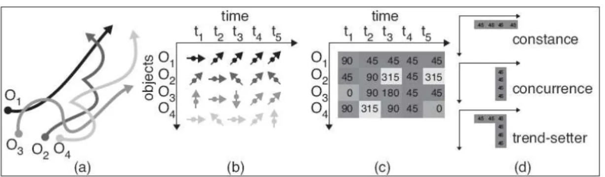
The method mentioned above are all using the coordinates, an alternative is by considering speed, an innate spatio-temporal variable. Laube et al. (2004) defined a collection of spatio-temporal patterns based on direction of movement and location, e.g. flock, leadership, convergence and encounter, and they proposed algorithms to compute them efficiently. These patterns are defined based on their previous study on REMO (Laube et al. 2002). The basic idea of the analysis concept is to compare the motion attributes of point objects over space and time, and thus to relate one object's motion to the motion of all others. The REMO concept (RElative MOtion) is based on two key features: First, a transformation of the lifeline data to a REMO matrix featuring motion attributes (i.e. speed, change of speed or motion azimuth); second, matching of formalized patterns on the matrix (Fig. 5).

The REMO concept allows construction of a wide variety of motion patterns. See the following three basic examples:

¾ Constancy: Sequence of equal motion attributes for r consecutive time steps (e.g. deer O1 with motion azimuth 45° from t2 to t5).

¾ Concurrence: Incident of n MPOs showing the same motion attributes value at time t (e.g. deer O1, O2, O3, and O4 with motion azimuth 45° at t4)

(39)

anticipates at t2 the motion azimuth 45° that is reproduced by all other MPOs at time t4)

Figure 5: The geospatial lifelines of four MPOs (a) are used to derive in regular intervals the motion azimuth (b). In the REMO analysis matrix (c) generic motion patterns are matched (d).

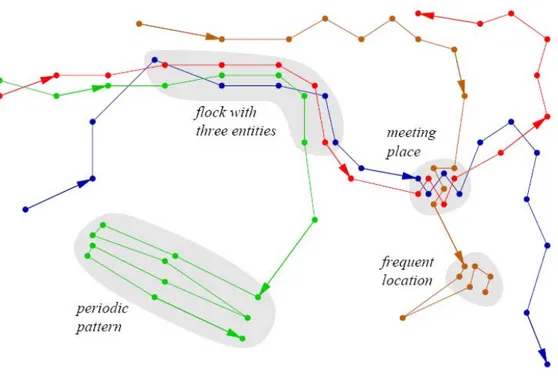
However, many sheep moving in a similar way is not enough to define a flocking pattern. We expect additionally that all the sheep of a flock graze on the same hillside. Formalized as a generic motion pattern we expect for a flocking the MPOs to be in spatial proximity. Adding spatial constraints to the list of basic motion patterns in figure 2, amended REMO patterns are listed as follows (Fig. 6).

¾ Track: Consists of the REMO pattern constancy and the attachment of spatial constraint. Definition: constancy + spatial constraint S.

¾ Flock: Consists of the REMO pattern concurrence and the attachment of a spatial constraint. Definition: concurrence + spatial constraint S.

¾ Leadership: Consists of the REMO pattern trend-setter and the attachment of a spatial constraint. For example the followers must lie within the range ( , ) when they join the motion of the trend-setter. Definition: trend-setter + spatial constraint S.

In addition, Laube et al. (2004) proposed the movement pattern convergence (Fig. 7) to answer questions similar to “Can we identify points of interest attracting people only at certain times, events of interest rather than points of interest, losing their attractiveness after a while?” Also noted that entities move towards the same location does not mean they will actually meet there. Thus another movement pattern encounter was also defined.

(40)

Encounter: Extrapolated meeting within R. Set of m MPOs at interval I with motion azimuth vectors intersecting within a range R of radius r and actually meeting within R extrapolating the current motion.

The opposites of the above described patterns are termed divergence and breakup. The latter term integrates a spatial divergence pattern with the temporal constraint of a precedent meeting in a range R.

Benkert et al. (2007) modified the original definition of a flock to be a set of entities moving close together during a time interval. Note that in this definition the entities involved in the flock must be the same during the whole time interval, in contrast to the moving cluster definition by Kalnis et al. (2005). Benkert et al. (2007) observed that a flock of m entities moving together during k time steps corresponds to a cluster of size m in 2k dimensional space. Thus the problem can be restated as clustering in high dimensional space. To handle high dimensional space one can use well-known dimensionality reduction techniques. There are several decision versions of the problem that have been shown to be NP-hard, for example deciding if there exists a flock of a certain size, or of a certain duration. The special case when the flock is stationary is often called a meeting pattern.

Andersson et al. (2007) gave a more generic definition of the pattern leadership and discussed how such leadership patterns can be computed from a group of moving entities. The proposed definition is based on behavioral patterns discussed in the behavioral ecology literature. The idea is to define a leader as an entity that (1) does not follow anyone else, (2) is followed by a set of entities and (3) this behavior should continue for duration of time. Given these rules all leadership patterns can be efficiently computed.

(41)

of trajectories considering only one controlling point, the ending point and starting point respectively. The difficulty now is the extrapolation needed for detecting convergence.

(42)

Figure 7: Geometric detection of convergence. Let S be a set of 4 MPOs with 7 fixes from t0 to t6. The illustration shows a convergence pattern found with the parameters 4 MPOs at the temporal interval t1 to t3. The darkest polygon denotes an area where all 4 direction vectors are passing at a distance closer than r. The pattern convergence is found if such a polygon exists. Please note that the MPOs do not build a cluster but nevertheless show a convergence pattern.

2.3.2 Spatio-temporal Association Rules

(43)

A STAR (ri, T1, q) =) (rj, T2) denotes a rule where entities in a region ri satisfying condition q during time interval T1 will appear in region rj during time interval T2. The support of a rule is the number, or ratio, of entities that follow the rule. The spatial support takes the size of the involved regions into consideration. That is, a rule with support s involving a small region will have a larger spatial support than a rule with support s involving a larger region. Finally, the confidence of a rule is the conditional probability that the consequent is true given that the antecedent is true. By traversing all the trajectories all possible movements between regions can be modeled as a rule, with a spatial support and confidence. The rules are then combined into longer time intervals and more complicated movement patterns.

Nanniet al.(2008) proposed the case of spatio-temporarily related traffic jams. For example, traffic jam (Pisa, 7.30 AM) traffic jam (Lucca, 8.30 AM), meaning that whenever the first event (a traffic jam in Pisa at 7.30 AM) occurs, usually it is followed by the second one (a traffic jam in Lucca at 8.30 AM). A more general version of this rule could be traffic jam (Pisa, t) traffic jam (Lucca, t+1 h), in which time appears as a parameter. Rules could also be discovered after even further abstracting time, as the following generalization shows traffic jam (Pisa) traffic jam (Lucca). In the same style of these examples, frequent patterns can be discovered in the trajectory data.

Researchers sticking to continuous space and time are trying to tackle with the continuity problem in two complementary ways by (1) considering patterns that are in the form of trajectory segments and searching approximate instances in the data and (2) considering patterns that are in the form of moving regions within time intervals, such as spatiotemporal cylinders or tubes – that, in some sense, represent a segment of trajectory plus a bounded approximation/uncertainty – and counting as occurrences all trajectory segments fully contained in the moving regions.

(44)

outputted as sequences of rectangles such that their width quantifies the average distance between each segment and the points in the trajectory it covers.

The second approach, based on moving regions, is followed by (Kalnis et al. 2005), and concerns the discovery of density-based spatial clusters that persist along several contiguous time slices. Finally, a similar goal, but focused on cyclic patterns, is pursued in (Mamoulis et al. 2004): the authors define the spatiotemporal periodic pattern mining problem (i.e. finding cyclic sequential patterns of given period) and propose an effective and fast mining algorithm for retrieving maximal periodic patterns. While time is simply assumed to be discrete, spatial locations are discretized dynamically through density-based clustering. Each time a periodic pattern is generated, in the form of a sequence of spatial regions, a check is performed to ensure that all regions in the pattern are dense – and then significant.

2.4 Conclusions

(45)

3 Preprocessing and Exploratory Analysis of data

In this chapter, the real data set from Starkey Project will be introduced along with basic background knowledge. Then the detail of data preprocessing will be included in the second section. At last, a first impression of the data set will be gained by exploratory spatio-temporal data analysis, where visualization techniques will be extensively used.

3.1 Starkey data set

3.1.1 Introduction of Starkey project

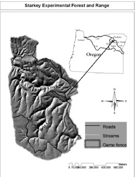
Starkey Experimental Forest and Range is located 35 km southwest of La Grande, Oregon, in the Blue Mountains of northeastern Oregon, USA. This 10,125-ha project area is enclosed by a 2.4-m high fence that prevents immigration or emigration of resident elk and other large mammals (Rowland et al. 1997). Starkey is divided into multiple subunits, the largest being a 7762-ha main study area where data for the current study were obtained (Figure 8). Starkey is situated at about 1500m elevation and supports a mosaic of coniferous forests, wet meadows and grasslands that typify summer range habitat for elk in the Blue Mountains. A network of drainages creates a complex and varied topography Details of the study area and facilities are available elsewhere (Johnson et al. 2000; Rowland et al. 1997).

Elk locations were obtained by an automated telemetry system that uses retransmitted LORAN-C radio navigation signals (Rowland et al. 1997). A subset of the Starkey telemetry data during the interval of May 2–May 28 in 1996 was selected for this study.

3.1.2 Trajectory data

(46)

Figure 8: The Starkey Project is located within the Starkey Experimental Forest and Range in the Blue Mountains, northeast Oregon.

(47)

Figure 9: Two elk tracks in May, 1996. The paths are sampled in time, hence the straight line segments.

Figure 9 provides an example of the tracks of two elks. An obvious difference can be observed between these two particular animals: the left one did not move too much over Starkey, but the right one visited widely spread locations all over Starkey.

(48)

3.1.3 Previous study on the dataset

There are plenty of studies on this project since 1988 encompassing every aspect such as animal behavior, ecosystem dynamics, distribution, human disturbance, statistical Modeling and so on. The research on movement patterns was mainly conducted by Haiganoush K. Preisler, Alan A. Ager and David R. Brillinger. Several interesting patterns were discovered by EDA and stochastic modeling.

First, a parallel box plot (figure 10) of the square roots of estimated elk speeds by hour of the day. The groups of animals appear substantially more mobile around 0500 hrs and 1800 hrs and less active at night and midday.

Figure 10: Parallel box plot of estimated elk speeds by hour of the day(Ager et al. 2003)

Secondly, figure 11 provides kernel density estimates of the animals’ noon locations based on all the data available. Noon was picked since, following Figure 3, the animals’ were less mobile then. There are several hot spots, i.e. locations of congregation, for the elk.

(49)

most habitat variables, but not all. Morning movements were uphill, towards more convex topography, and at increasing distance to streams. Afternoon movements were directed towards easterly aspects, steeper slopes in valley landforms, and towards streams. At dusk, movements were strongly upslope, out of drainages, and towards areas that are characteristic of foraging areas, i.e. lower canopy cover, greater distance to hiding cover, increased herbage production, closer to roads, and more southerly and westerly aspects.

Figure 11: Kernel density estimates of elks at noon during spring(Ager et al. 2003)

(50)

movement vectors, these being distance to security areas, distance to foraging meadows, distance to steep slopes, and distance to streams. On the other hand, movements that are seemingly random, like foraging paths in a meadow, or movements that cannot otherwise be explained with environmental covariates are included as stochastic terms in the model. The reader is referred to Brillinger et al. (2004) and Preisler et al. (2004) for details.

3.1.4 Elk

The elk (Cervus elaphus), is one of the largest species of deer in the world and one of the largest mammals in North America and eastern Asia. Elk range in forest and forest-edge habitat, feeding on grasses, plants, leaves, and bark.

Some important facts relevant to movement patterns are listed as below(RMEF 1999):

¾ Food, water, shelter and space are essential to elk survival.

¾ Female elks, baby elks and yearlings live in loose herds or groups.

¾ Male elks live in bachelor groups or alone.

¾ During the rut, female elks and baby elks form harems with one or two mature male elks.

¾ In cold snowy climates, female elks, baby elks and young male elks migrate to foothills and valleys in winter.

¾ In spring, male elks begin to migrate first to higher elevations than female elks and young elk. Female elks often begin migrating before they give birth to their baby elks, which are typically born in late May through early June. They stop to give birth and allow their young to grow for several weeks. By late June or July, they've resumed moving into higher country where they will find rich summer food.

¾ An experienced elk, usually the lead female elk, guides a herd between seasonal ranges.

3.2 Data preprocessing

(51)

other focal operators: an important parameter for analysis but also a major influence as a smoothing filter. This observation is significant in movement research in that often little information is provided about trajectory data models and algorithms employed in computing movement descriptors in a particular study. In order to increase the transparency and the repeatability of analysis of movement trajectories, so how their trajectory descriptors are computed is reported in detail.

3.2.1 Data selection and data cleaning

The main task of data selection is to determine a subset of the records or variables in the database for focusing the search for interesting patterns.

Based on the previous extensive studies on elk trajectories, tracks of 59 elks during spring 1996 were selected at the beginning for two reasons: first the movement of elks was most intensively sampled in 1996, second elks are less active in summer season while requires finer scale study, but both the spatial and temporal accuracy cannot suffice the demands. Furthermore, since the samples were collected temporally uneven, the distribution along monitoring period was studied (Figure 12). As a result, the subset from 2 May to 28 May (shown in the bounding rectangle) of samples was selected.