Determinants of Outstanding Mortgage
Loan to Value Ratios:
Evidence from the Netherlands
∗
M. Ricardo Cunha, Bart M. Lambrecht and Grzegorz Pawlina
December 17, 2009
Abstract
This paper studies the determinants and behavior of outstanding mortgage loan to value (LTV) ratios for a panel data set of 5,179 households over the period 1992-2005. We find that outstanding LTVs are driven by household character-istics, life-cycle effects and mortgage type characteristics. LTV declines with the time elapsed since mortgage commencement, but its level is consistently higher (by around 10%) for non-repayment mortgages (such as interest-only or endowment mortgages) than for repayment mortgages (such as linear or annuity mortgages). The difference results from higher debt capacity associated with the possibility of deferring the principal repayment for non-repayment mortgages. Our results indicate that the recent proliferation of non-repayment mortgages is driven by tightening financing constraints due to declining affordability in the housing market and that the overall quality of outstanding mortgages has substantially deteriorated over the last decade.
Keywords: housing finance; mortgages; leverage choice (JEL: C21, D14, G21)
∗Cunha is from Portuguese Catholic University, Porto, and gratefully acknowledges financial
sup-port for his doctoral studies from Fundacao para a Ciencia e Tecnologia. Lambrecht and Pawlina are from the Department of Accounting and Finance, Lancaster University, UK, and thank the ESRC (grant RES-062-23-0078) for financial support. We also thank participants of EFA (Bergen), AREUEA (Istanbul), BAA (Blackpool), Maastricht-MIT-Cambridge Real Estate Finance and In-vestment Symposium, Portuguese Finance Network conference (Coimbra), and Warsaw Interna-tional Economic Meeting for helpful comments and suggestions. Correspondence can be sent to g.pawlina@lancaster.ac.uk.
For a number years we have witnessed an increase in homeownership rates and in the amount of aggregate mortgage debt both in the US and across the world (e.g., Li (2005) and OECD (2006a)). The very easy access to credit and the proliferation of more flexible mortgage products have made mortgages available to households that would not be able to afford a house a few decades ago.
The recent rise in home foreclosures and the ’subprime’ mortgage crisis have, how-ever, drawn attention to a number of worrying developments and trends in mortgage lending. In particular, there has been a notable increase in recent years in lending to high-risk, so-called subprime, borrowers as well as a rise in non-performing mort-gages (see Demyanyk and Van Hemert (2008)). Loan incentives such as ‘interest-only’ mortgages, low initial ‘teaser’ rates, repayment holidays and laxer lending criteria are frequently cited as having encouraged borrowers to take on more debt than they can handle.
The situation in the housing market has a considerable effect on the whole economy. The aggregate value of the owner-occupied housing stock in the US increased from $2.8 trillion in 1982 to $7.3 trillion in 1999 (see Case (2000)), which is comparable with half of the American stock market capitalization. Consequently, any wave of households entering into negative equity, resulting bankruptcies and forced sales would all feed back into the stability of the financial system, consumer demand and, in general, economic growth itself. A proper understanding of the riskiness of household mortgage debt is therefore key to assessing measures and designing policies aimed at preserving the stability of the economic growth. Since mortgages are secured by the value of the house, the mortgage credit risk is in the first instance determined by the ratio of the outstanding mortgage debt to the value of the house, commonly known as the loan-to-value (LTV hereafter).1
The academic literature has, however, devoted surprisingly little attention to the analysis of outstanding LTV. To quote Follain (1990) in his presidential address to the AREUEA: ”Although much has been written about the aggregate demand for mortgages, housing economists do not seem to have picked up on what many finan-cial economists have made a career of doing – explaining debt-equity ratios.”2 In his 1Von Furstenberg (1969) was one of the first to show that the loan-to-value ratio governs the level
of default rates over the life of the mortgage. He found that reducing the downpayment in the highest LTV range by as little as 1% of home value can cause default rates to rise by 50%. More recently, Demyanyk and Van Hemert (2008) show that in the run-up to the mortgage crisis high LTV borrowers became increasingly riskier compared to low LTV borrowers.
2The few exceptions include Englund, Hendershott, and Turner (1996), who study the effect on 2
presidential address to the AFA, Campbell (2006) states that household finance is an underresearched area and he points out the lack of good quality data as one of the main reasons.
This paper aims to address this gap and presents an empirical study on housing finance. As detailed international micro-level data of housing finance is not readily available, we test our hypotheses using a detailed survey data from the Netherlands. As we motivate later, the characteristics of the economic and legal framework in the Netherlands allow us readily to generalize many of our conclusions to other countries (see Guiso, Sapienza, and Zingales (2008), who use data from the same survey). Our paper addresses the following questions. What are the determinants of LTV for home-owners who have outstanding mortgage debt? How does LTV vary over a household’s lifecycle? How has the proliferation in recent years of mortgages without compulsory amortization (such as ‘interest-only’ mortgages) affected LTVs and what are their long-term consequences for LTV ratios? What are the characteristics of households that choose a mortgage product without compulsory amortization and have they changed over time? And, finally, are higher LTV ratios and repayment flexibility reflected in mortgage interest rates?
While there is vast theoretical and empirical evidence that corporations follow some optimal leverage level, we find that for households outstanding LTV declines as the time from mortgage commencement elapses. Amortization of the mortgage debt is one obvious reason. Appreciation in the value of the house may be another one. There appears to be little or no evidence that the initial LTV at mortgage commencement is anything like an intertemporal optimum that households seek to maintain. Moreover, the dispersion in outstanding LTVs is quite large (especially compared to the variation in corporate leverage ratios). A histogram of outstanding LTV ratios in our study reveals that the average LTV of households with outstanding mortgage debt in our sample is 0.497 with a standard deviation of 0.270. Importantly, more than 15% of the homeowners in our sample do not have any outstanding mortgage debt.
What explains this wide dispersion of outstanding LTV across homeowners? We find a pronounced life-cycle effect in LTV in that LTV declines with the time elapsed
housing finance of financial deregulation in Sweden during the 1980s based on data on loan-to-value ratios for homeowners that moved recently, and Hendershott and Pryce (2006), who report a sub-stantial decline in LTVs following the abolishment of mortgage interest relief for taxation purposes in the UK. In a related work, Koijen, Van Hemert, and van Nieuwerburgh (2008) investigate the choice between the adjustable and fixed rate mortgages.
since mortgage commencement. Furthermore, we identify a number of other determi-nants of LTV. The number of household members is shown to positively affect LTV, whereas a household’s net worth (total assets minus total outstanding debt) negatively influences it. This latter effect follows from the fact that households with low net worth are more likely to be financially constrained and may have to rely more heavily on debt financing. Households on social benefits and those facing a higher tax rate also exhibit a higher LTV.
We also show that the mortgage type adopted is an important explanatory variable of outstanding LTV, with non-compulsory repayment contracts being associated with higher levels of debt. One explanation for this may be that the reduction in the out-standing mortgage debt is primarily determined by a compulsory amortization schedule for repayment mortgages, whereas repayment of outstanding debt is left to the discre-tion of the borrower in the case of non-repayment mortgages. More surprisingly, the wedge in LTV between both mortgage types remains even if one adjusts non-repayment mortgages for the cash value of the savings that have been accumulated in special in-vestment vehicles linked to the mortgage. A striking trend during our sample period is the dramatic increase in the mortgage to income ratio, especially for non-repayment mortgages.
The combination of higher LTV and substantially higher loan-to-income ratios for ’non-repayment’ mortgages indicates that these mortgages are potentially riskier than repayment mortgages. This finding is consistent with the fact that the recent surge in mortgage defaults in the US and the UK has been linked primarily to mortgages that share many of the features present in non-repayment mortgages. Why then have so many households chosen to adopt non-repayment mortgages in recent years? We investigate the households propensity to select a non-repayment type mortgage (as opposed to a repayment mortgage) using a binary choice (probit) model and show that the proliferation of non-repayment mortgages has been driven primarily by the dramatic decline in housing affordability.3 This is consistent with the observation that
over the period of our sample the house price index (HP I1994 = 100) rose from 80 in
3There may, of course, be other reasons for the proliferation of non-repayment mortgages that we do
not capture in our study. For example, mortgage brokers typically receive a higher commission on non-repayment type mortgages and may therefore have incentives to oversell these products. Examples of this behavior are the reported cases in the UK of ‘endowment’ mortgages that were sold to borrowers for whom this product was inappropriate. These cases prompted an investigation by the Financial Services Authority, who subsequently tightened up the UK code of mortgage lending practice in order better to protect borrowers against this type of misselling.
1992 to 280 in 2005, whereas house affordability (as defined in Appendix A) declined from about 117 in 1992 to about 50 in 2005. Another important reason for the increased popularity in non-repayment mortgages is the tax advantages they confer. Our findings indicate that non-repayment mortgages relax financing constraints and help households to catch up (in the short run at least) with the soaring house prices.
The remainder of the paper is organized as follows. Section 1 discusses empirical hypotheses, Section 2 presents the data set, whereas Section 3 describes the main trends in the Dutch housing market. Section 4 focuses on the univariate analysis, which is followed by the regression analysis of Section 5. Section 6 concludes.
1
Hypotheses
While firms and households show many similarities, they are also different in a number of ways. Unlike corporations, households have finite horizons and are likely to be risk-averse. Therefore, we postulate that the household financing decisions are the outcome of the interplay of factors that affect their demand for financing as well as the ability to service debt. Some of the factors are expected to parallel those of corporations, such as net worth, income or education (serving as a proxy for both financial sophistication and the future income generating ability). The other factors we consider are specific to households. Age is expected to be one of key determinants of leverage because the level of mortgage debt tends to decline along the life cycle. Finally, variables such as the number of household members and the degree of urbanization determine the demand for housing so they are likely to affect the LTV ratio as well. Our first empirical hypothesis is therefore:
H1: The LTV ratio is a function of socio-demographic variables, such as income, net worth, education, household size, location as well as the stage in the household’s life-cycle.
Mortgage contracts analyzed in our study differ predominantly with respect to repayment flexibility. We classify mortgages into ‘repayment’ mortgages and ’non-repayment’ mortgages. The former are defined as mortgages that have a compul-sory amortization schedule (such as ‘annuity’ and ‘linear’ mortgages) and the latter as mortgages that leave discretion with respect to the amortization schedule (such as ‘interest-only’ mortgages and ‘endowment’ mortgages).4 As the mortgage choice
flects a household’s preferences for repayment flexibility, we put forward the following hypothesis:
H2: Flexible mortgages are associated with higher LTV ratios throughout the life of the mortgage.
One obvious motivation for this hypothesis is the fact that the reduction in the out-standing mortgage debt is primarily determined by a compulsory amortization schedule for repayment mortgages, whereas repayment of outstanding debt is left to the discre-tion of the borrower in the case of non-repayment mortgages. In addidiscre-tion, households who select non-compulsory repayment mortgages self-select to do so and, therefore, are likely to value (and to use) the flexibility their contracts are associated with.
To address the evolution of the LTV rates over time and the associated prolifera-tion of the non-compulsory repayment mortgages, we test three addiprolifera-tional hypotheses. First, we point out that it is not always obvious whether a higher LTV implies riskier mortgage debt. Both i) the higher LTV level and ii) the proliferation of flexible (i.e., with no compulsory repayment of the principal) contracts may also be a result of sophisticated optimizing investors shifting to the flexible products once they become available in the market. Households on a high income may, for example, adopt flexible non-repayment mortgages because of tax considerations. Our hypothesis is therefore: H3a: Households adopt flexible contracts in order to exploit the advantages of debt, such as tax savings.
If the non-compulsory repayment contracts are chosen by financially sophisticated households, then their proliferation and the (resulting) higher LTVs are a sign of a rational response of optimizing agents to the emergence of new products. For financially sophisticated households, variables such as education and income will have a positive effect on the probability of selecting flexible mortgages and on the levels of LTV, as they indicate a higher level of wealth and financial sophistication. Moreover, the differences
the outstanding loan and a fixed percentage of the total loan. On the other hand, with an ‘interest-only’ mortgage one pays interest during the term of the mortgage and a large ‘balloon’ payment at the end. Other mortgages covered by our study are ‘traditional life-insurance’ mortgages, ‘improved life-insurance’ mortgages, ’investment’ mortgages, ‘annuity’ mortgages and ’life-insurance’ mortgages. The various mortgage types covered in our study are discussed in more detail in Section 3.4. Definitions of each mortgage type can also be found in the Appendix B. Note that the typical distinction between fixed rate and variable rate mortgages is less important in the Netherlands because the overwhelming majority of mortgages are fixed rate mortgages.
between the characteristics of borrowers choosing standard and flexible contracts should prevail over time. If these are financially sophisticated households who choose the flexible, high LTV products, then the proliferation of non-repayment contracts will generally not be associated with higher credit risk.
The alternative hypothesis is that the flexible contracts (and higher LTV) are mostly selected by financially constrained households, who – otherwise – would not be able to afford a house. In such a case, the proliferation of flexible contracts and the increase in average LTV would be an indicator of higher credit risk.
H3b: Households adopt flexible contracts to alleviate financing constraints.
If the alternative hypothesis H3b is true, then measures of financial constraints are the main determinants of the mortgage type choice. The choice of higher leverage and non-compulsory repayment contracts will be unrelated to marginal tax rates and will not depend (or will depend negatively) on the measures of financial sophistication (such as education). The total pool of mortgage contracts will become more risky over time as the households with worse characteristics follow the wealthier and more sophisticated ones in choosing non-repayment contracts.
Our final hypothesis is related to the potential cost of leverage and of repayment flexibility.
H4: The interest rate increases with the LTV ratio and is higher for non-repayment mortgages.
Households who decide to borrow more or to select a non-compulsory repayment contract may face an upward sloping supply curve of mortgage loans, which translates into higher borrowing rates. In equilibrium, some households may find it optimal to accept higher mortgage interest rates as a price for the benefits of higher borrowing and for the flexibility embedded in the non-repayment contracts. The alternative hypothesis is that higher LTV ratios and flexible contracts are not associated with higher interest rates. If flexible mortgages come at no additional cost, then rational borrowers may prefer them to traditional contracts. This may lead to a proliferation of non-repayment mortgages.
2
Data
The data set used is based on the DNB Household Survey (DHS) carried out by Cen-tERdata, a data collection unit of the Center for Economic Research at Tilburg Uni-versity (see also Guiso, Sapienza, and Zingales (2008)). The (rotating) panel covers the period 1992-2005, containing end of the year data for a yearly average of over 1000 representative households in the Netherlands, and provides very unique information about the financing, spending, labor and social decisions of individual households. Ob-servations considered are the ones in which all relevant parts of the questionnaire were answered by household members.5 The sample therefore comprises 13,546
household-years (9,422 owners, 4,124 renters), 7,860 of which being borrowers (5,731 with non-repayment and 2,129 with non-repayment contracts). For descriptive analysis purposes, the sample is divided in 4 periods (1992-1995, 1996-1998, 1999-2002, and 2003-2005). Households responding to all parts of the questionnaire in several years are consid-ered as different observations. In the regression analysis, we control for the potential correlation of error terms within a household.
All currency-denominated values are expressed in euro (using the official NLG/e 2.20371 conversion rate), and are in real terms. Inflation correction was made through-out the period for all currency denominated variables, considering the Consumer Price Index (CPI) as deflator. The reference year considered is 1994 (CP I1994 = 100).
Data collection for households and individuals involves several challenges, mainly due to privacy and refusal issues. Still, our data set contains a significant number of observations, a representative demographic spread and a good coverage of the main household variables, such as housing, assets, liabilities, and personal information. Fur-thermore, an exhaustive categorization within these classes of variables is available, in particular for housing and mortgage variables. Thus, we can assume our sample to be ”of quality”, according to the requirements postulated in Campbell (2006).6
Finally, the economic and legal factors that influence homeownership and housing finance are fairly homogenous across the Netherlands (unlike the United States or Germany, for example, where legislation, taxation and financial policy may vary across 5We removed extreme outliers as well as implausible observations from the data. The following
criteria led to the omission of an observation from the sample: total asset value abovee5m, net income value abovee2m, mortgage interest rate above 20%, house value above e2m, LTV ratio above 1.5, and the age of the eldest member of the household (in years) above 100.
6Bucks and Pence (2006) demonstrate the reliability of household surveys by providing empirical
states). Furthermore, the LTV behavior in the Netherlands have been less distorted by incentives problems of lenders and financial intermediaries. Unlike the US, the practice of passing on credit risk through mortgage securitization is still comparatively rare. As a result incentive and monitoring problems have not been as severe. This is one of the reasons why lending standards have not been loosened as much over time. We believe for the above reasons that the Netherlands is particularly suitable for investigating this paper’s research questions (see also Charlier and van Bussel (2003)).
3
Trends and determinants of housing finance
3.1
General trends
The reported percentage of owner-occupied homes in the Netherlands in 1990, 1994, 1998, 2000, 2002 and 2006 were respectively 45.3%, 47.6%, 50.8%, 52.2%, 54.0% and 54.2% (Ministry of Housing (2002) and CBS).7
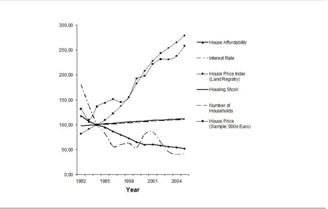
The increase in the total housing stock has been very modest. Figure 1 shows that the housing stock has merely kept pace with the rising trend in the number of households. The number of households increased from 6.266 million in 1992 to 7.091 million in 2005, whereas the corresponding numbers for the housing stock are 6.043 and 6.912 million, respectively. In contrast, the house price index (HPI) constructed by the Dutch land registry office has risen from 81 in 1992 (with HP I1994 = 100) to
a spectacular 279 in 2005. This translates into an annual growth rate of about 10%. Furthermore, household income has risen at a much lower pace causing the affordability ratio in 2005 to be less than half its 1992 level. The OECD (2004) reports that housing affordability in the Netherlands (defined as the proportion of available income to house price value) declined more than anywhere else, except for Spain, during the period 1991 to 2002. Brounen, Neuteboom, and van Dijkhuizen (2006) predict that housing affordability in the Netherlands (with an average spending of more than 35% of income 7The reported rates are, however, still among the lowest in the European Union. The reason is that
traditionally the Netherlands have not had a large owner-occupied housing sector. The Dutch govern-ment policy, particularly during the first half of the 20th century was very much focused on stimulating the construction of social housing. However, since the early 90s the Netherlands housing policy has observed a shift, and the main housing policy objective is to promote affordable owner occupation (Ministry of Housing (2002)). Taxation schemes, guarantees, bureaucratic and economic incentives have been implemented as means to promote homeownership. Also, incentives to the conversion of dwellings in the vast social rental scheme to owner occupied dwellings have been introduced.
on housing by the end of 2007) will deteriorate more than in any other European country.
[Insert Figure 1 about here]
While affordability has fallen to a record level, interest repayments as a fraction of disposable income have not increased by as much. The reason is that interest rates have fallen dramatically over the sample period (from 9.27% in 1992 to 2.09% in 2005).8 Record low interest rates have provided households with access to cheaper
credit allowing them to lever up their income aggressively in order to keep up with rising house prices. This is reflected in the substantial increase in the loan-to-income ratio (see section 3.3).
With regards to our data, homeownership rates in the sample are somewhat higher than the rates for the Netherlands as a whole. Table 1 shows that owner occupancy rates in our sample are 71.7%, 68.7%, 67.0%, and 67.8% for the respective four periods.9
About 3% of households in the total sample own a second house, but this proportion has been declining from 3.7% in the first sample period to 1.7% in the last sample period.
[Insert Table 1 about here]
Table 1 also shows that the average initial loan-to-value (i.e. at the time of mortgage commencement) has fallen from 80.3% to 75.2% over the period of study. Average 8The 1992 interest rate refers to the Guilder Market Interest Rate, whereas the 2005 rate refers to
the Eurozone Interest Rate.
9There are a number of potential reasons why observed ownership rates are higher than the ones
observed in the official statistics. It is likely that our sample does not adequately include certain segments of the population that typically do not own their home. For example, homeless or very poor people are under-represented in our sample. Also households that are highly mobile or do not have a fixed residence are less likely to be included in our survey. Elderly people who have sold their home to pay for a room in a care-home would neither appear in our sample. These are all people who typically are unlikely to own their home. Finally, single person households are significantly under-represented in our sample. Since the homeownership rate is substantially lower for this group (only 42%) this creates another upward bias in our ownership rates. We conclude that higher availability of information on housing issues for homeowners may therefore lead to a bias in the questionnaire response rates towards the observed higher proportion of homeowners.
outstanding loan-to-value of households has dropped from 44.4% to 39.9%. If we take out households without a mortgage then the average loan to value has dropped from 52.9% in the first period to 44.8% in the third period, only partially bouncing back in the last period to 48.2%. The drop in outstanding loan-to-value ratios have to be interpreted, however, in the context of inflated house prices, the spectacular rise in loan-to-income ratios and trends in various other determinants of LTV. In fact, our regression analysis in next section shows that, when controlling for other effects, there is a positive time trend in outstanding LTV.
3.2
Household balance sheet and income: Owners vs. renters
Table 2 shows the balance sheet for the average homeowner and non-homeowner house-hold. The data are reported in an analogous way as for public corporations whenever possible. Although we have detailed data for assets and liabilities, developing an income statement for households is not possible as information about household consumption and expenses is not disclosed in our data set.10
[Insert Table 2 about here]
Starting with homeowners’ assets, the balance sheet shows that the house counts for 75.7% of the assets of the average household in the total sample. Another 1.4% and 3.5% are to be attributed to a second house or other real estate investments, respectively. Cash accounts and cash savings together account for another 7.6%. In-surance policies, financial market based savings, money lent and other savings together count for about 7.2%. Vehicles count for 3.9%. Total assets for homeowners amount to e205,860 on average. In contrast, total assets for non-homeowners are only e22,128 on average. In the absence of real estate the asset portfolio is much more weighted towards savings and financial investments. Cash accounts and cash savings together count for 49.2%. Insurance policies, financial market based savings, money lent and other savings together count for another 31.3%. Vehicles make up the remaining 19.5%.11
On the liability side household equity (net worth) counts for 66.1% for homeowners in the full sample. Consequently, the majority of households assets has been financed 10For a detailed analysis of household portfolios and their international comparisons, see Guiso,
Haliassos, and Jappelli (2002).
11The above proportions have been fairly constant over time, except that financial market based
by retained income, accumulated wealth, or money transfers such as endowments, donations or inheritance. The mortgage on the house counts for 30.1%. In comparison, the other financing sources are negligibly small. The analysis of external housing finance can therefore safely be restricted to mortgage financing. More than 80% of house owners finance their property using a mortgage. This fact is consistent with the Income Panel Survey (IPO, Inkomens Panelonderzoek ), and with the findings of Alessie, Hochguertel, and van Soest (2002) in their analysis of household assets and liabilities portfolios in the Netherlands.
Net worth of non-homeowners counts for 88.1% of all liabilities. 5.6% of assets are financed by short-term extended lines of credit (4.8%), overdrafts (0.6%) or credit cards (0.2%). Medium term financing (mainly private and study loans) count for another 4.5%. Loans from family and friends and other loans count for the remaining 1.8%.12
Home-owning households in our sample have an average total salary ofe30,837, an average gross income ofe42,595, and an average net income of e29,197. For households that do not own their home these values are substantially lower and respectively given by e18,324, e26,596 and e18,917. In our regression analysis we use adjusted income equivalence values according to the number of household members, which represent a better relative earning position of the household. The equivalence is computed using the Eurostat scale, which considers the first household member with a factor 1, the second 0.5, and any additional member 0.3. The equivalence values are then equal to per capita values where the number of household members is calculated according to the relevant scale.13
[Insert Table 3 about here]
3.3
Housing finance structure
Dutch house prices have boomed since the start of our period of analysis. In our sample, average house values rise substantially too during the period of observation. Although our data reflect house values perceived by households and not actual transaction values, research has shown that house values reported by survey respondents are fairly reliable 12The composition of liabilities has remained fairly stable over time. Mortgage financing has declined
somewhat in favor of net worth.
and accurate (see, e.g., Bucks and Pence (2006)). The average real house value for our sample over the full period of study is e171,613, and grew from e135,104 in the 1992-95 period to e242,426 in the 2003-05 period. As can be seen from Figure 1, our average sample house values are in line with the house price index.
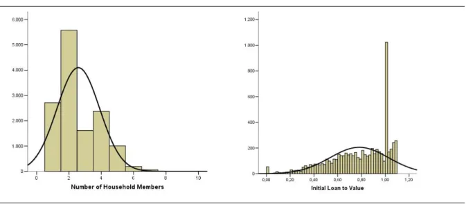
Figure 2 (Panels B-D) shows frequency histograms of the average initial loan to values (ILTV) and the average loan to values during the periods under consideration.14
[Insert Figure 2 about here]
Table 4 documents the evolution of loan-to-income ratios for repayment and non-repayment mortgages. While for non-repayment mortgages the ratio remains fairly constant around 1.4, the ratio rises for the increasingly ubiquitous non-repayment mortgages from 1.71 in 1992 to 2.99 in 2005.
[Insert Table 4 about here]
The data shows a clear link between outstanding LTV and age. The average out-standing LTV for homeowners below the age of 35 is 0.62. This fraction falls approx-imately by 0.1 for every 10 years of age that is being added, leaving over 65 year old homeowners with an average outstanding LTV of 0.19. Note that between 80% to 90% of all homeowners up to the age of 65 have a mortgage, but only 65% of owners over 65 have a mortgage. This sudden drop can be explained by the fact that mortgages usually have a 30-year term in the Netherlands.
3.4
Mortgage types
Table 5 provides information on the various mortgage types in our data. The definition of each mortgage type is included in Appendix B. As previously explained mortgage types have been divided into two categories: repayment mortgages and non-repayment mortgages. Mortgage types falling into the former category are annuity mortgages and linear mortgages, whereas the latter category includes the various types of life-insurance mortgages, endowment mortgages, investment mortgages and interest-only mortgages.
14When computing the descriptive statistics, we removed observations with an initial loan-to-value
of less than 0.1 or more than 1.1. Outstanding loan-to-value observations are not affected by this data selection, and hence no effect from this procedure is found in the regression results of Section 4.
[Insert Table 5 about here]
Table 5 reports the frequencies for each mortgage type in our sample, as well as the average loan-to-value for each mortgage type. We consider both initial loan-to-values (i.e., upon mortgage commencement) and the loan-to-values at the time of the survey. Mortgages with a compulsory repayment component accounted for 36.0% of all mortgages at the start of the sample period. This number had fallen to 12.9% by the end of the sample period. Life insurance mortgages (and its variants) accounted for 47.3% at the start of the sample period, and had dropped to 32.3% for the last period. Most noticeable is the spectacular rise of pure interest-only mortgages which do not feature in a specific category for the first two periods, but amount to 36.6% of all mortgages in the last period.
Interestingly, average initial loan-to-value in our sample has been consistently be-tween about 70% and 80% for all types of mortgages. Cases of initial loan-to-value close and above 100% do occur, however, as legally no initial loan-to-value limit is imposed in The Netherlands.15 Interest-only mortgages, dominant in the last years of the sam-ple, have lower average initial loan-to-values than other mortgage types. Possibly, the absence of compulsory capital repayments (or any other associated investment vehicle that can act as collateral), and the lower collateral for the lender compared to other mortgage types, leads to a higher initial down-payment requirement as a guarantee.
As to be expected, the evolution of the loan-to-value over time varies dramatically across mortgage types: average LTVs decline much faster for repayment mortgages than for those mortgage types that do not have a compulsory repayment of the principal. Average LTVs for the former category are more than 40% lower than the initial LTV (e.g. the average LTV for annuity mortgages drops from 80% at commencement to 40% at the time of the survey). For the latter category this drop is within the range of 20% to 35% and the ultimate repayment of the principal when the mortgage expires (or if the housing market were to enter in a recession) remains therefore much more uncertain.
The existence of a lower loan to value and faster repayment for compulsory repay-ment mortgages is true even if one deducts the cash value of life insurance policies from the outstanding debt in life-insurance type mortgages (life insurance, traditional life insurance, and improved traditional life insurance mortgages).16
15In practice 125% is, however, considered an upper bound by most lenders.
16In our data set this insurance policy value is reported since 2000. For households reporting
Given that mortgages without a compulsory repayment have become much more prevalent in recent years this may have implications for future homeownership. In particular, when the mortgage expires (typically by the time the mortgagee retires, considering the usual 30 year maturity of mortgages in the Netherlands) some of the less wealthy households may have to sell off the property in order to pay off the out-standing debt. Unless a new and smaller house is bought this may lead to a drop in homeownership rates for households that are retired. Brounen and Neuteboom (2006) estimate however that this pressure in homeownership will not be as pronounced as initially expected. In light of the recent US mortgage crisis it should also be noted that mortgages with a higher outstanding LTV may be more exposed to a recession in the housing market.
The increased popularity of non-repayment mortgages may, in part, be due to the tax advantages they confer. Until 1997 interest from all types of household debt (mort-gage debt and the different consumer debt types) was tax deductible. Between 1997 and 2000 a phasing out process of the deductibility of consumer debt interest and mort-gage interest not associated with the primary residence was implemented. Since 2000 interest tax deductibility has been confined to the main loan used for purchase (and maintenance) of the primary residence but, unlike most other countries, the total de-ductible value is uncapped. However, interest on consumer debt, mortgages on second homes and on mortgage equity withdrawals are disqualified for tax-shield purposes. The new tax policy therefore makes mortgage debt more attractive than other forms of credit and puts investors in real estate at a disadvantage compared to first-time buyers. Taxation policy has had an effect on the choice between mortgages with compulsory and non-compulsory principal repayment. Official evidence shows that the concession of tax benefits and guarantees for house owners coincided not only with an increase in owner occupied housing, but also with a wave of re-mortgaging and a shift to more interest-based mortgages (Ministry of Housing (2002)). This latter effect is observed in our sample and was described above. Finally, towards the end of our sample period the banking industry created numerous financial products combining mortgage tax shields and capital gains concessions, which observe high popularity.17
6.5% and 7.2% of the total value of the house, respectively, in periods 1999-02 and 2003-05, to which correspond an average corrected loan to value of 0.47 and 0.49. These corrected loan to value figures are substantially higher than the ones observed for mortgages with compulsory repayment.
17In the Netherlands capital gains on personally held assets are not taxed. However, taxable returns
on capital assets are set at a presumptive rate of 4% of the value of the assets, and taxed at a 30% rate. This taxation scheme is however not valid for owner occupied real estate, where concessions are made
The government’s homeownership policies, increased banking competition and eas-ier access to mortgage debt (e.g. by considering dual income for credit scoring pur-poses) had not only an effect on homeownership rates, but were also key factors in the evolution of house prices (Brounen, Neuteboom, and van Dijkhuizen (2006)).
4
Univariate analysis
To analyze the outstanding mortgage loan to value ratio of households, it is important to recognize that the LTV is only defined for those households that own their home. It is therefore important first to analyze what differentiates homeowners from renters. In this section we define and analyze a number of variables that are traditionally con-sidered to be important determinants of homeownership. We use a univariate analysis and non-parametric tests to explore whether homeowners are inherently different from renters in terms of their characteristics.
Next we focus on the housing finance decision. As will be shown later, the type of mortgage contract adopted (that is, ”repayment” mortgage contract versus the flexible “non-repayment” mortgage) has important implications for the level and evolution of the outstanding mortgage LTV. We postpone the explicit modeling of a household’s outstanding LTV till later and explore in this section what differentiates homeowners that choose a repayment mortgage from those that adopt a non-repayment mortgage. For this purpose we perform a univariate analysis similar to the one that compares owners with renters.
We start off by defining the main explanatory variables used in this study (for all variable definitions, see Appendix A). These variables include a mix of income related, socio-economic, demographic and geographic variables that traditionally are considered to be important determinants of homeownership and the housing finance decision.
The existing literature identifies household income as an important determinant of homeownership (Linneman and Wachter (1989)) and housing finance (Hendershott and Pryce (2006)). We define the variable IN COM E as the combined gross income of all household members adjusted for the number of household members using the
as part of the national housing policy. Taxation on owner occupied housing assets is done through the calculation of an estimated rental value of 1.25% of the value of the house minus mortgage interest, making investment in real estate (financed by mortgage debt) for owner occupancy more attractive relative to other assets. For a detailed discussion of the taxation scheme in the Netherlands, see Cnossen and Bovenberg (2001), and Rele and van Steen (2001).
Eurostat equivalence scale.18 As the maximum mortgage loan advanced by lenders is often a multiple of household income, income therefore determines whether (and how much) the household receives mortgage debt in the first place. Moreover, at the time of initiating the mortgage a higher income to house value ratio implies a stronger potential to pay off the house purchased. This allows households to adopt a higher initial LTV. While this positive effect may be mitigated by high income households having a higher capacity to repay debt more quickly, we would expect the effect of the higher initial LTV to dominate.
To capture household wealth, we introduce N ET W ORT H, which is the difference between the net worth and the estimated house price appreciation since its purchase. All else equal wealthier households have the choice between converting their net worth into liquid assets to finance the house or, alternatively, to keep (or spend) those assets and to finance the house by debt. Households with little net worth, on the other hand, have no other option but to finance the house by debt. Wealth constraints may therefore induce a negative relation between net worth and the LTV.
We separately introduce the variable BEN EF IT , previously not used in the lit-erature. This variable comprises unemployment, sickness and disability benefits ad-justed for the number of household members using the Eurostat equivalence scale. While social benefits are a source of income, they also signal that the household may be experiencing difficulties (such as unemployment, incapacities or illness) that could adversely affect homeownership propensity. The effect of benefits on the financing de-cision is therefore ambiguous. On the one hand, while benefits are a source of income, lenders may categorize it as ’low quality’ income against which it may be more difficult to borrow. Moreover, households are less likely to own a house. Very often, on the other hand, households may become recipients of benefits after they have taken out a mortgage (as result of redundancy or accidents). In that case the household’s capacity to service the debt may, ex post, be substantially diminished making it more difficult to reduce LTV. BEN EF IT is expected to have an overall positive marginal effect on LTV.
18We use income values that are adjusted for the number of household members, as this gives a
better measure of the relative earnings position of the household. The equivalence is computed using the Eurostat scale, which considers the first household member with a factor 1, the second 0.5, and any additional member 0.3. The equivalence values are then equal to per capita values where the number of household members is calculated according to the relevant scale. For a detailed discussion of this and other used income equivalence scales see OECD (2006b).
T AX is defined as the estimated effective tax rate equal to the ratio of the tax bill (the difference between the gross and net income) and the tax base (the difference between the gross income and the estimated mortgage interest). Households with a higher tax rate also have a higher potential tax shield. Interest on mortgage debt is tax deductible (whereas rent is not). Furthermore, capital gains on the household’s residence are tax exempt. The tax deductability of mortgage interest should increase the expected outstanding mortgage debt. Furthermore, theory predicts (see Henderson and Ioannides (1983)) that a higher, more progressive tax rate stimulates homeown-ership because there is a bigger financial advantage from owning versus renting. The positive effect of taxation on homeownership should further strengthen this positive relation. The existing literature (e.g. Hendershott and Pryce (2006)) argues that taxes may have an effect on outstanding LTV. All else equal, a household with a higher tax bill has a higher potential tax shield and may want to adopt more debt over its life cycle. Variable T AX captures the estimated effective tax rate faced by a household and is predicted to have a positive relation with LT V .
We define D M EM 2 and D M EM 3 as dummy variables taking the value of 1 for households with exactly two and at least three members, respectively, and zero otherwise. We expect that D M EM 2 and D M EM 3, as well as AGE, the age of the oldest household member expressed in years, positively affect both the probability of homeownership as well as LTV (the later being a result of a preference towards ceteris paribus a bigger, thus more expensive, house). As retired households sometimes move into homes for the elderly or convert the equity in their home into cash for consumption, the relation between the probability of homeownership and AGE may, however, be non-monotonic. D EDU is a dummy variable taking value of 1 for tertiary or vocational education and zero otherwise. The effect of this variable (if any) remains an open question. Furthermore, we introduce D U RBL, a dummy variable equal to 1 if the household lives in an area with a low degree of urbanization and 0 otherwise.19
AF F measures affordability and is defined as the ratio of the average income in the province of household i in year t (as reported by the CBS and standardized for the 19The Central Bureau of Statistics (CBS) in the Netherlands uses a measure of address density in
a particular area to measure the degree of urbanization. The degree of urbanization is expressed in 5 categories going from ‘very high’ degree of urbanization (code 1) with a density of more than 2,500 addresses per square kilometer, to a ‘very low’ degree of urbanization (code 5) with less than 500 addresses per square kilometer. The same convention is used in our data – the degree of urbanization takes on the discrete values between 1 and 5, covering the spectrum from ‘very high’ to ‘very low’. Our dummy variable D U RBL equals one for urbanization levels 3 to 5, and zero otherwise.
number of household members) to the average value of the house in that province (as reported by the Dutch land registry office). RCO captures the (inverse) relative cost of ownership and is defined as the ratio of the average rent to the average house value in the province of household i in year t. T Y P E represents the type of dwelling, and is equal to 1 for a single family home, 2 for appartment/flat, and 3 for all other cases (such as shared accommodation).
Finally, IN T denotes the difference between the mortgage interest rate of household i and the prevailing market interest rate in year t.
We now first explore whether renters are inherently different from homeowners in terms of their characteristics. To test the null hypothesis that both samples (i.e., renters and homeowners) are drawn from populations with the same distribution (the same mean) for the various characteristics, we use the Mann-Whitney test (the t-test). We find overwhelming evidence against the null hypothesis over the whole sample period for pretty much all household variables considered.20 This shows that the characteristics of
renters and homeowners are fundamentally different. Using a t-test for the equality of means, we find that homeowners exhibit higher average net worth (e103, 527 for owners compared toe21, 608 for renters), enjoy higher income (e25, 033 versus e17, 630), are more highly educated (0.67 versus 0.57), are subject to a higher average tax rate (0.30 versus 0.25), have higher affordability ratio (0.12 versus 0.11). Homeowners also receive lower social benefits than renters (e966 versus e1, 659). On the demographical side, home-owning households are larger on average (eg. 45% have 3 or more family members, whereas the corresponding percentage for renters is 24%). Homeowners also live in less highly urbanized areas (with an average of 0.66 for the urbanization dummy variable for owners and 0.44 for renters) and enjoy bigger houses (a house type indicator equal to 1.20 and 1.54 for owners and renters, respectively). All these differences are significant at the 1% level. The analysis of subsamples corresponding to the first and the last sample periods indicates that the qualitative differences between homeowners and renters prevail over time as most of the differences that are significant in the initial period (period 1) are significant in the final period (period 4) and also over the entire sample period.21
[Insert Table 6 about here]
20Exceptions are the variables AF F , D M EM 2 and AGE for which the null hypothesis cannot be
rejected in every sample period.
21Again, the exceptions are AF F , D M EM 2 and AGE, for which the difference is not always
The second key question we address in this section relates to the type of mort-gage financing that homeowners are using. In particular, we compare the holders of repayment mortgages with those who opted for a non-repayment mortgage. Table 7 compares the characteristics of repayment mortgageholders and non-repayment mort-gageholders over the total sample period, for period 1 and for period 4 (1992-1995 and 2003-2005, respectively).
Focussing on period 1 first, the Mann-Whitney test provides strong evidence that both sub-samples are very different with respect to most explanatory variables (ex-cept for the degree of urbanization, and the relative cost of owning versus renting). The t-tests for the means provides evidence that in the first period more flexible non-repayment mortgages are chosen by households with higher income (e30, 653 versus e26, 426 for owners with a repayment mortgage), which are more highly educated (0.71 versus 0.66) and subject to a higher tax rate (0.35 versus 0.34). In addition, non-repayment mortgage holders are younger (46.08 years versus 49.24 years), live in bigger houses (1.15 versus 1.25), which are more affordable (0.15 versus 0.14), have lower (in-verse) relative cost of ownership (2.8 versus 2.82) and receive less social benefits (e753 versuse1, 303). Moreover, non-repayment mortgages are associated with higher mark-ups on market interest rates (2.38 versus 1.86). All the differences are significant at a 1% significance level for the means as well as distributions (apart from RCO, for which the difference in means is significant at the 5% level and the difference in distributions is not significant). These results suggest that the more financially ”sophisticated” households (cf. Campbell (2006)) tend to choose the more flexible, though more ex-pensive, non-repayment mortgage to optimize dynamically their financing structure.22 Consequently, the evidence obtained so far indicates the higher LTV associated with non-repayment mortgages does not necessarily translate into higher risk.
This picture changes quite dramatically in the final period where the distributional differences between the two groups are no longer statistically significant (even at a 10% significance level) for important variables such as income (IN C), affordability (AF F ), the type of housing (T Y P E), the (inverse) relative cost of ownership (RCO) and the degree of urbanization (D U RBL). Furthermore, households choosing non-repayment mortgages are now on average less highly educated (0.69 and 0.77), contrary to the situation observed in the initial sample period. Their tax rate is higher only at 10% 22The lower net worth of the households choosing flexible mortgages (e82, 729 and e89, 705) is
not inconsistent with this view as by choosing non-compulsory repayment mortgages and deferring payments, they avoid the need of reducing today’s consumption.
significance level and benefits are lower at a 5% level. Finally, the differences in age and net worth retain the same sign and similar statistical significance.
The univariate analysis of the two groups of borrowers indicates that initially more flexible, non-repayment contracts are selected mainly by financially sophisticated households, who do not face particular financing constraints (as their incomes are on average higher) but who are willing to optimize dynamically their financing structure (to maximize the utility of their lifetime consumption by, e.g., deferring repayments and minimizing the tax liability). However, towards the end of the sample period the differences in the characteristics of households diminish or even disappear. The loss of the discriminatory power of the key variables indicates that non-repayment mort-gages have to a large extent substituted compulsory repayment contracts through the entry of below-average quality households to the group of flexible borrowers. As a consequence, the riskiness of mortgage pool has increased and the higher LTV ratios of flexible mortgage holders are likely to reflect financing constraints and not necessarily the optimizing behavior with respect to the financing structure.
The results for the whole sample period provide a mixed picture for the obvious reason that the composition of the pool of borrowers choosing non-repayment mort-gages changes over time, as we just explained. The comparison of the two groups of borrowers across the entire sample period reveals that households with non-repayment mortgages have generally lower net worth, lower age, are subject to a lower tax rate, live in a more highly urbanized areas, but also in bigger houses, while enjoying higher income and lower social benefits (see Table 7).
[Insert Table 7 about here]
Our previous conclusions with respect to the increased riskiness of non-repayment mortgages over time are based on the implicit assumption that non-repayment mort-gages exhibit a higher LTV ratio. In fact, this assumption is supported by the data. A comparison of the average LTV ratios across the two major types of mortgage contracts indicates a growing gap between LTVs of non-repayment and repayment contracts over the sample period. In particular, the average gap in years 2003-2005 (period 4) equals 0.52 − 0.25 = 0.27, and exceeds the corresponding value for years 1992-1995 (period 1) amounting to 0.59 − 0.43 = 0.16.
5
Regression analysis
We model empirically the following economic problem. Each household can make an irreversible decision to buy a house.23 The decision is only going to be made if a latent
variable (a function of a number of economic, demographic and geographical vari-ables) exceeds a certain level. As we are not able to observe the entire history of each household (nor have an exact economic model for the value of the latent variable), the ownership regression is aimed at explaining the maximum historical propensity to own a house using a household’s current characteristics. Financing decisions are assumed to be made continuously, in the sense that a household can freely choose the level of leverage at each point throughout its house tenure. However, the type of mortgage fi-nancing is selected only once – when the (first) mortgage is initiated. Furthermore, any contractual restrictions on the level of leverage for compulsory repayment mortgages, which are inherent to this type of financing products, are viewed as just one of the fac-tors contributing to the level of leverage (and are captured by a dummy characterizing the mortgage type).
Define OW N∗ to be the variable corresponding to the (unobserved) historical max-imum of the propensity to own a house, with OW N∗ > 0 equivalent to a household finding it optimal to buy their home at some point in the past. LT V∗ is the current borrowing propensity and reflects the desired loan-to-value ratio. We are interested in estimating the following relationships:
(
OW Nit∗ = X1itα + εit
LT Vit∗ = X2itβ + ηit,
(1) where Xjit, j ∈ {1, 2} is a vector of explanatory variables, parameters α and β denote
vectors of model coefficients and εit (ζit) is the error term drawn from a bivariate
normal distribution with mean 0 and variance σε2 (σζ2). The covariance between both error terms is σ12, which can be different from zero. Subscripts i and t correspond to
a household and a year, respectively.
As OW N∗ and LT V∗ describe preferences, which are not observable, we define two new variables:
23In our sample, only 105 households, i.e., 2% of total number of households decided to reverse the
decision and moved to a rented property. Moreover, there are 335 cases of households changing their mortgage type.
OW Nit≡ ( 1 if OW Nit∗ > 0 0 if OW Nit∗ ≤ 0 (2) and LT Vit≡ LT Vit∗ if LT Vit∗ > 0 and OW Nit∗ > 0 0 if LT Vit∗ ≤ 0 and OW Nit∗ > 0 Not observed if OW Nit∗ ≤ 0. (3)
Consequently, OW N is a binary variable describing homeownership and LT V is the current loan-to-value ratio of a household that owns a home (therefore, LT V is only observed in the group of owners).
In the described model, only the sign of OW N∗ is observed and LT V is observed only when OW Nit∗ > 0. The vector of explanatory variables, X1it, is observed for
all data points and X2it may not be known for those observations for which OW N∗
(or even LT V∗) is negative. The first equation in (1) is the selection equation as it corresponds to the household’s self-selection into the group of homeowners. The second equation is the regression equation.
We analyze the ratio of the outstanding mortgage loan to the value (LTV) for households that have selected to own a property and decide to borrow a strictly positive amount. The modeling approach that most closely reflects the spirit of a household’s decision problem is a double-hurdle regression model (Cragg (1971)). The model allows for the absence of borrowing to be a result of i) the absence of homeownership, or ii) the decision to finance the property entirely with equity. As data requirements for the double-hurdle model are the most stringent, we also estimate Heckman sample selection (cf. Amemiya (1984), see also Li and Prabhala (2006)) and OLS models with a richer set of explanatory variables.
The double-hurdle specification is the one consistent with the system of equations (2) and (3) but it requires that the vectors of explanatory variables (X1 and X2)
be observed for the entire sample. As some of the explanatory variables of interest (e.g., mortgage type) are not observed for a fraction of observations (renters), the double-hurdle model can be estimated only with a subset of explanatory variables. To circumvent this limitation, we also estimate the Heckman sample selection model, which does not require that X2 be observed for those households that do not self-select to the
group of owners. The disadvantage of using Heckman specification is that it assumes that the explained variable in the regression equation (LT V ) is always positive if the
household belongs to the group of owners.24 As such, it ignores the second possibility in equation (3), that is, that homeowners adopt a 100% equity financing. To make sure that our conclusions are not affected by the exclusion of the group of owners which are non-borrowers, we estimate a tobit model using the subsample of owners. While ignoring sample selection issues (by not taking account the third possibility in (3)), such a specification allows for including homeowners with no outstanding mortgage debt. Unfortunately, the tobit specification also requires that X2 be observed also for
those households who do not borrow, which puts similar restriction on the feasible set of explanatory variables as the double-hurdle model. Therefore, we also estimate a conditional OLS model of LTV for households that select to borrow a strictly positive amount. This model allows us to use the full set of the explanatory variables and does not require making specific assumptions about the reason for the exclusion from the group of the borrowers (negative propensity to borrow or non-participation in the housing market).25
The interpretation of the regression parameters and the corresponding marginal effects depends on the exact model specification. For the double-hurdle, Heckman and tobit models, it reflects the effect of the exogenous variable on the (unobserved) propen-sity to borrow. For the OLS model, it reflects the corresponding effect on the observed LTV conditional on the household having a mortgage loan outstanding. To see the differences between the estimated coefficients, consider the following example. Assume that household income affects positively both the propensity to own a house and the propensity to borrow and that the corresponding regression error terms, which repre-sent unobserved factors affecting the propensities, are positively correlated. Regression coefficients of the double-hurdle, Heckman and tobit models will be the estimates of the true parameter βinc. However, the coefficient of the OLS model reflects the effect
of income conditional on the selection to the sample of borrowers. In the analyzed example, the conditional marginal effect is smaller than βinc. This is due to the fact
that ceteris paribus the expected LTV is higher if the household is included among the owners, which is the result of a positive correlation between the two error terms. If 24In our sample, this assumption is violated for 1,562 observations, for which homeownership is not
associated with the presence of mortgage financing. As a result, those observations are omitted when the Heckman model is estimated.
25As the OLS estimator based on a model with truncated data is generally biased when sample
selection is not random, see Greene (2000), pp. 902-903, we also calculate the conditional marginal effects based on the sample selection model. The estimated effects (available upon request) are in line with those obtained for the OLS model.
the level of the explanatory variable increases, the magnitude of the shock needed for the household to be included in the group of owners becomes smaller. As a smaller (positive) error term in the selection equation is associated with a smaller expected error in the LTV equation, the increase of the expected LTV (conditional on selection to the group of borrowers) following the marginal change in income is lower than the true model coefficient.26
Finally, in the second part of the analysis, we define the following variable to in-vestigate the choice of mortgage category:
D N RP M Tit≡ 1 if N RP M Tit∗ > 0 and min{LT Vit∗, OW Nit∗} > 0 0 if N RP M Tit∗ ≤ 0 and min{LT V∗ it, OW N ∗ it} > 0
Not observed if min{LT Vit∗, OW Nit∗} ≤ 0,
(4) D N RP M T is therefore a dummy variable equal to 1 if a household has a non-compulsory repayment mortgage and 0 otherwise, and N RP M T∗ denotes the (un-observed) propensity to select a non-compulsory repayment mortgage. Model (4) is estimated using the sample selection probit (Heckman probit) approach. The model is therefore based on the same principle as the standard Heckman model with the only difference being that the explained variable in the regression model is binary (here – mortgage category). The selection equation in the estimated Heckman probit is the same as the selection equation of model (1).27
5.1
Results
We begin with the results of the simple model of LTV, which is formulated as follows 26The effect in tobit model will be affected in the same way as in the Heckman and double-hurdle
models with positively (negatively) correlated error terms and identical (opposite) signs of the coeffi-cients of the relevant variable in the selection and regression equation. In such a case, the conditional effects will be of a smaller absolute value. If in a Heckman or a double-hurdle model the positively (negatively) correlated error terms are combined with opposite (identical) signs of the coefficients in the selection and regression equation, then the conditional marginal effect will (in absolute terms) be greater.
27To estimate model (4) using Heckman probit with selection equations as in (1), we essentially
LT Vit∗ = β0+ β1SQRT IN Cit+ β2SQRT N ET W ORT Hit+ β3SQRT BEN EF ITit
+β4T AXit+ β5T AXit∗ D AF T 97 + β6D M EM 2it+ β7D M EM 3it (5)
+β8AGEit+ β9AGEit2 + β10D EDUit+ β11Y EARit+ β12D U RBLit+ ηit.
Recall that the propensity to borrow, LT V∗, is defined as the (desired) ratio of the current value of the mortgage outstanding and the market value of the house. When implementing model (5), we use LT V , given by (3), as LT V∗ is generally not ob-servable.28 The choice of most of the explanatory variables has been motivated in
Section 4. In addition, SQRT IN C, SQRT N ET W ORT H and SQRT BEN EF IT are introduced and denote square-root transformations of IN C, N ET W ORT H and BEN EF IT , respectively.29 To capture the possible effect of the tax regime shift we also introduce the interaction dummy D AF T 97 that equals 1 for period 1998-2005, and zero otherwise. Variable Y EAR corresponds to the year number and is defined as the actual year number minus 1992. This variable should capture a possible time trend in household leverage that results from factors that cannot be controlled for, such as governmental policies (aimed, e.g., at promoting homeownership), proliferation of mortgage products or, more generally, changes in credit market conditions.
It is important to stress that we are not modeling the household’s initial (i.e., at mortgage commencement) loan-to-value, but the outstanding loan-to-value at the time of the survey. It is more challenging (and more general) to model the latter than the former. For example, while the former is primarily determined by lending policies and borrowers’ financing constraints, the latter is also affected by household life-cycle effects, past income and liquidity shocks. As such the possible variation in outstanding LTV is typically much larger than the variation in initial LTV. Obviously, initial LTV is a special case of outstanding LTV (if households are surveyed immediately after mortgage commencement, then the outstanding LTV coincides with the initial LTV).
[Insert Table 8 about here]
28We performed a robustness check of the reliability of the reported house values by estimating
model (5) for subsamples with varying maximum time since mortgage commencement. We did so to verify whether there is any systematic bias in reported house values that may increase with the time elapsed since house purchase. We found that our results are not particularly sensitive to the choice of the maximum time since mortgage commencement allowed in the sample.
29The square root is a commonly used transformation in demographics research (see Goodman
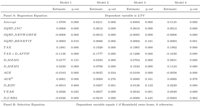
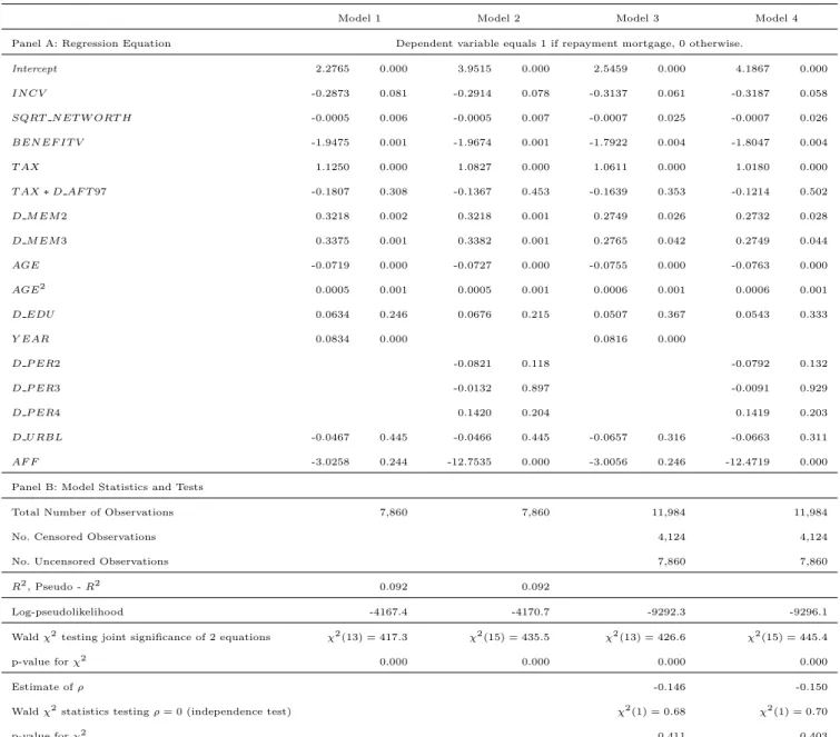
The results of the LTV regression model (5) are reported in Table 8 and gener-ally confirm hypothesis H1 about the relevance of socio-economic variables. The sign of the relationship between LT V and income is positive and significant for all model specification. Depending on the specification, an increase of income bye10,000 trans-lates for the average borrowing household (with income e25,350) into an expected increase in LTV ratio between 0.025 and 0.039 (depending on the model specification). The positive relation indicates a higher debt capacity of high-income households. Net worth (N ET W ORT H) has a strong negative effect on outstanding LTV: less wealthy households have no other choice but to take on more debt. An increase of e10,000 reduces expected leverage by 1-2 percentage points for the mean borrowing household, which has a net worth of e84,797. Social benefits increase LTV – the estimate of the net economic effect of an extra euro of social benefits on LTV ranges between 3 and 9 percentage points. The amount of taxes paid has a significantly positive (prior to 1997) but economically rather modest effect on LTV. A 1% increase in the effective tax rate leads to an increase in LTV by 0.16-0.20 percentage points. The relationship loses its statistical significance after 1997, that is, when tax relief on interest is phased out, except for interest on mortgage debt.
Leverage increases with the number of household members. A second member adds on average between 0.017 and 0.085 to LTV, which is slightly lower than the estimated effect of any higher number of members (between 0.023 and 0.112). The marginal effect of age varies (based on Model 1 in Table 8) from −0.012 for AGE = 20 to −0.008 for AGE = 40 and −0.005 for AGE = 60. Education positively influences the propensity to borrow (the estimates range from 0.013 to 0.023) and significantly affects the observed LTV (as indicated by p-value in the conditional OLS model). The estimate of the effect of calendar time ranges from 0.26 to 0.57 percentage points per year. This time effect reflects the autonomous change in the levels of household leverage that can be attributed to the changes in regulation and in the level of credit supply.
Finally, the negative coefficient of the low-level urbanization dummy (which ranges from not significant to −0.034) indicates that the level of urbanization may positively influence the observed LTV ratio. This result is consistent with housing in more ur-banized areas being less affordable and, as such, requiring a higher proportion of debt financing.
The estimated parameters of the sample selection equation (Table 8, Panel B) are in line with the analysis of the determinants of homeownership in Section 4 and, to a large extent, with the literature (see, e.g., Goodman (1988), Zorn (1989), Jones
(1989), Haurin, Hendershott, and Wachter (1997) and Coulson (2002)). Namely, the probability of homeownership is positively affected by income, net worth, education, and the estimated tax rate. Furthermore, consistent with the results of the univariate analysis, households having more members and who live in larger homes situated in less highly urbanized areas are more likely to belong to the group of owners. Contrary to the results of Section 4, social benefits do not seem to be a statistically significant determinant of homeownership. Also, the coefficient of affordability has a negative sign (this result may to same extent capture the non-linearity of the time trend).
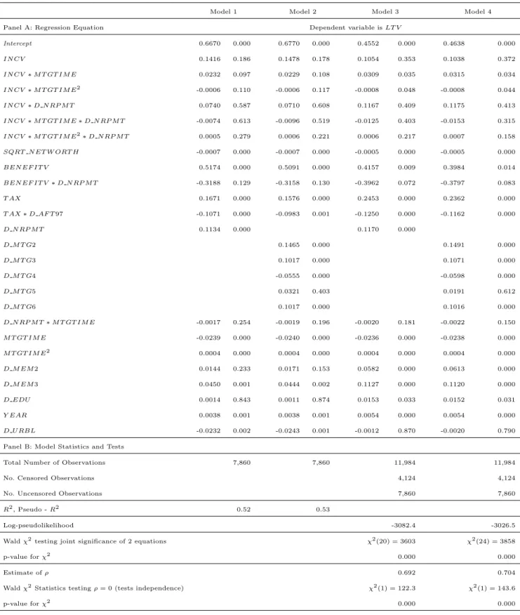
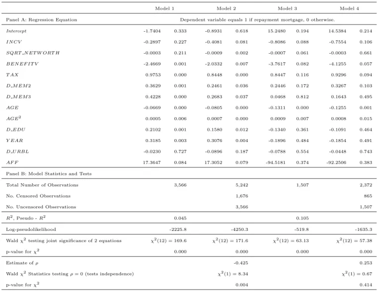
Having analyzed the model of choice based on a basic set of explanatory variables, we proceed to a richer specification that takes into account the characteristics of the outstanding mortgage contracts. Our descriptive statistics indicate that the type of mortgage financing chosen (payment versus non-repayment mortgages) may have a persistent, long-term effect on the evolution of LTV. The mortgage type is fixed when the mortgage is initiated and, as such, an exogenous variable. We denote the mortgage type by the dummy variable D N RP M T (where D N RP M T = 1 for non-repayment mortgages, and zero otherwise).30
We predict that the choice of mortgage type determines the effect of income on the outstanding LTV. While income positively affects the initial LTV level, for non-repayment mortgages this effect is likely to be higher for the following reasons. The possibility of deferring the repayment of the principal implies that non-repayment mortgages support a higher initial LTV ratio. Moreover, the resulting higher interest payment allows for more significant tax deductions.
Furthermore, the time elapsed since mortgage commencement (which we denote by M T GT IM E) certainly effects LTV. Households, unlike firms, have a natural, finite lifetime. The income generating power of households is limited in time, and therefore also its capacity to service debt. It seems therefore unrealistic to impose the assump-tion that households maintain some inter-temporal optimal LTV ratio. This is the main motivation for introducing the variable M T GT IM E in the regression, as well as M T GT IM E2, to allow for non-linearities.
We allow the marginal effect of income to depend on M T GT IM E, the time elapsed since mortgage commencement (to capture life-cycle effects), and also on D N RP M T , 30It is worth pointing out that since the late nineties it has become easier and relatively cheaper for
households to remortgage and therefore to change the mortgage type. Still, among 7,860 borrower-years, there are only 335 occurrences of a mortgage type change. Those changes are usually associated with an increase of the level of debt.