WORKING PAPER SERIES
Universidade dos Açores
CEEAplA WP No. 19/2006
Determinants of Length of Stay: A Parametric
Survival Analysis
António Gomes de Menezes
Ana Isabel Moniz
Determinants of Length of Stay: A Parametric
Survival Analysis
António Gomes de Menezes
Universidade dos Açores (DEG)
e CEEAplA
Ana Isabel Moniz
Universidade dos Açores (DEG)
e CEEAplA
Working Paper n.º 19/2006
Novembro de 2006
CEEAplA Working Paper n.º 19/2006
Novembro de 2006
ABSTRACT
Determinants of Length of Stay: A Parametric Survival Analysis
Length of stay is one of the most important decisions made by tourists as it
conditions their overall expenditure and stress caused on local resources. This
paper estimates survival analysis models to learn the determinants of length of
stay as survival analysis naturally lends itself to study the time elapsed between
arrival and departure at a destination. It is found that individual
sociodemographic profiles, such as nationality and gender, and attributes of
actual trip experiences, such as repeat visitor behavior and overall satisfaction,
are important determinants of length of stay. Thus, this paper’s regression
results can be used to estimate the probability that a given group of individuals
experiences a stay longer than a given threshold. This is important to the design
of marketing strategies that effectively influence length of stays.
Keywords: Length of Stay; Tourism Demand Modelling; Survival Analysis.
António Gomes de Menezes
Departamento de Economia e Gestão
Universidade dos Açores
Rua da Mãe de Deus, 58
9501-801 Ponta Delgada
Ana Isabel Moniz
Departamento de Economia e Gestão
Universidade dos Açores
Rua da Mãe de Deus, 58
9501-801 Ponta Delgada
Determinants of Length of Stay: A Parametric Survival Analysis November 2006
Determinants of Length of Stay: A Parametric Survival Analysis
António Gomes de Menezes University of the Azores
Department of Economics and Management Rua da Mãe de Deus
9501-801 Ponta Delgada Portugal E-mail: [email protected] Tel: +351-296650084 Fax: +351-296650083 Ana Moniz
University of the Azores
Department of Economics and Management Rua da Mãe de Deus
9501-801 Ponta Delgada Portugal
E-mail: [email protected] Tel: +351-296650084
Fax: +351-296650083
António Gomes de Menezes (corresponding author), PhD in Economics from Boston College, USA, is Assistant Professor in Economics, at the Uni-versity of the Azores and Research Associate at CEEAplA, Azores, Portugal, and Research A¢ liate at Fondazione Rodolfo Debenedetti, Universitá Boc-coni, Milan, Italy ([email protected]).
Ana Moniz, PhD in Management from the University of the Azores, is Assistant Professor in Management, at the University of the Azores and Research Associate at CEEAplA, Azores, Portugal.
Determinants of Length of Stay: A Parametric Survival Analysis
Abstract
Length of stay is one of the most important decisions made by tourists as it conditions their overall expenditure and stress caused on local resources. This paper estimates survival analysis models to learn the determinants of length of stay as survival analysis naturally lends itself to study the time elapsed between arrival and departure at a destination. It is found that individual sociodemographic profiles, such as nationality and gender, and attributes of actual trip experiences, such as repeat visitor behavior and overall satisfaction, are important determinants of length of stay. Thus, this paper’s regression results can be used to estimate the probability that a given group of individuals experiences a stay longer than a given threshold. This is important to the design of marketing strategies that effectively influence length of stays.
Keywords: Length of Stay; Tourism Demand Modelling; Survival Analy-sis.
1
Introduction
Length of stay is an important determinant of the overall impact of tourism in a given economy. The number of days that tourists stay at a particular destination is likely to influence their expenditure, for instance, as the number of possible experiences to be undertaken by tourists depends on their length of stay (Davies and Mangan 1992; Legoherel 1998; Kozak 2004). Understanding the determinants of length of stay is, thus, important to fully characterize tourism demand and its impact on a given touristic destination (Gokovali, Bahar and Kozak 2007). In addition, Alegre and Pou (2006) argue that the importance of uncovering the determinants of length of stay and concomitant gains to policymakers and researchers alike has grown with the increasingly pervasive pattern of shorter lengths of stays. Alegre and Pou claim that uncovering the microeconomic determinants of length of stay is critical to the design of marketing policies that effectively promote longer stays, associated with higher occupancy rates and revenue streams. In fact, income from tourism might well be falling in many destinations despite the increase in visitor arrivals, due to a decrease in the length of stay. Length of stay has also aroused interest beyond its importance as an expenditure determinant. For instance, in the tourism sustainability literature, length of stay is important in the context of carrying capacity analysis (Saarinen 2006). However, and as Gokovali, Bahar and Kozak (2007) argue, there are relatively few studies that estimate the determinants of length of stay resorting to microeconometric techniques. This paper contributes to fill this gap. The main aim of this paper is to estimate the determinants of length of stay, in particular, how different individual sociodemographic profiles and trip experiences influence length of stay. Length of stay is one of the questions resolved by tourists when planning or while taking their trips (Decrop and Snelders 2004). Hence, it follows that length of stay is best recorded when tourists depart, and, quite likely, is influenced by tourists’ sociodemographic profiles, on the one hand, and their experiences while visiting their destination, on the other (Decrop and Snelders 2004; Bargeman and Poel 2006). This paper accounts for such insights by employing micro data, rich on individual sociodemographic characteristics and actual trip experiences, built from individual surveys answered by a representative sample of tourists departing from the Azores: the Portuguese touristic region with the highest growth rate in the last decade.
Modelling length of stay poses certain challenges that owe to the fact that length of stay is, necessarily, a non-negative variable. To uncover causal relationships between tourists’ sociodemographic characteristics and trip experiences and length of stay, the empirical work must employ some sort of a formal statistical model. However, the most popular statistical tools, such as the linear regression model, are not appropriate to model length of stay, since they do not take into account that length of stay is a non-negative variable, and, hence, lead to biased estimation (Greene 2000). To circumvent such problem, this paper employs survival analysis parametric models in a novel way. This paper argues that survival analysis, or time to event analysis (read, departure), naturally lends itself to the study of length of stay. Quite interestingly, this paper employs a plethora of survival analysis parametric models that display much welcomed features. First and foremost, the survival analysis parametric models accommodate for individual heterogeneity, in the sense that a large number of covariates, pertaining to individual sociodemographic profiles and actual trip experiences, are used to explain length of stay, as suggested by microeconomic theory and a reading of the literature (Decrop
and Snelders 2004). It should be noted that controlling for individual heterogeneity allows detailed policy implications, as one is able to quantify the impact of specific individual characteristics or trip attributes on the probability of length of stay exceeding a given threshold for a synthesized, policy relevant individual or target group. Second, the survival analysis parametric models employed are unrestricted and agnostic in the sense that they allow for non-normal data patterns, such as spiky or bimodal data. This is especially important since some lengths of stays are more frequently found in the data than others, such as seven day stays.
Recently, and not surprisingly, several authors have employed microeconometric models to analyze the determinants of length of stay that explicitly deal with the limited nature of length of stay, namely, being a non-negative variable. Alegre and Pou (2006) employ a limited dependent variable discrete choice model, namely, a binary logit, and, thus, collapse length of stay into a binary variable: 0 if length of stay is shorter than one week; 1 if otherwise. By doing so, the ensuing policy implications are less far reaching, in the sense that all length of stays, say, shorter than one week are treated alike, be them one day stays or six day stays. This lost of information may be particularly worrisome when length of stays are not obviously dichotomized or clustered, and are, instead, roughly evenly distributed over several days, leaving the researcher with no obvious cut-off to arbitrarily partition length of stays. To avoid this problem, Gokovali, Bahar and Kozak (2007), like this paper, employ survival analysis parametric models to estimate the determinants of length of stay for a sample of tourists departing from a Turkish touristic region. While innovative and informative, the work by Gokovali, Bahar and Kozak is restricted to models of the Proportional Hazards form, and, therefore, with constant or monotone hazard rates: intuitively, the rate at which stays are terminated. This paper capitalizes on Gokovali, Bahar and Kozak yet employs a more general and, concomitantly, richer approach. In particular, this paper employs models not only of the Proportional Hazards form, as in Gokovali, Bahar and Kozak, but also of the Accelerated Failure-Time form, with the former being a special, nested case of the latter. This distinction matters since, and in a nutshell, the Proportional Hazards models, by construction, exhibit constant or monotone hazard rates. The Accelerated Failure-Time models, however, display no such restriction, and, hence, accommodate more general data patterns. This distinguishing feature is especially important in the present context since length of stays may exhibit spiky, multi modal patterns, depending on the destination or the time period under analysis. It should also be noted that this paper’s approach leads, ex ante, to models with a better fit to the data. In fact, since the Proportional Hazards models are, in a formal statistical sense, nested cases of Accelerated Failure-Time models, this paper employs a model selection strategy estimating both Proportional Hazards models and AcceleratedFailureTime models -that clearly dominates a model selection strategy -that estimates only the special case Proportional Hazards model. This turns out to be case, as expected. In fact, the econometric work carried out in this paper selects an Accelerated Failure-Time model as the preferred model, despite the fact that the Proportional Hazards models do display quite satisfactory statistical results.
The empirical work carried out in this paper produced statistically significant and economically important results. Several sociodemographic individual characteristics and trip attributes turn out to be statistically important determinants of length of stay, and, carry, thus, important policy implications. In fact, the results
uncovered may be used to aid the design of marketing policies that may promote longer stays. In addition, there are results that shed light on enduring research topics, such as repeat visitor behavior. In fact, it should be noted that repeat visitors display higher probabilities of experiencing longer stays, a fact in line with the findings in Lehto, O’Leary and Morrison (2004), who claim that repeat visitors exhibit extended length of stays.
This paper is organized as follows. Section 2, the body of the work, reviews the literature, describes the contextual setting and the data used in the econometric work, discusses the econometric model and comments the results. Section 3 concludes.
2
Determinants of Length of Stay: A Parametric Survival
Analy-sis
2.1
Literature Review
Length of stay is one of the most useful dimensions used to characterize tourism demand: an enduring research topic (for extensive reviews of research on tourism demand see, among others, Crouch 1994; Witt and Witt 1995; Lim 1997; Crouch and Louviere 2000; Song and Witt 2000). Tourism demand is a broadly defined subject that encompasses a variety of objects, interesting in their own right: tourist arrivals, tourist expenditure, travel exports, nights spend in tourist accommodations and length of stay. Length of stay is an interesting research topic for, at lest, two reasons. First, length of stay conditions the overall socioeconomic impact of tourism in a given economy. In fact, and as Davies and Mangan (1992) and Kozak (2004), among others, argue, an increased length of stay may allow tourists to undertake a larger number of experiences or activities which may affect their overall spending, sense of affiliation and satisfaction. Hence, several authors consider length of stay an important market segmentation variable in estimating the determinants of tourist spending (Davies and Mangan 1992; Legoherel 1998; Mok and Iverson 2000). Second, modelling length of stay is important to tourism sustainability analysis (Saarinen 2006). Sustainability has recently become an important policy issue in tourism. The ubiquitous continuous growth of tourism has fuelled an intense discussion about the socioeconomic and environmental impacts that tourism hinges on destination areas. In the sustainability literature, an important concern focuses on destination areas’ carrying capacity, generally defined as the maximum number of people who can use a site without any unacceptable alteration in the physical environment and without any unacceptable decline in the quality of the experience gained by tourists. The concept of carrying capacity occupies a key position with regard to sustainable tourism, in that many of the latter’s principles are based on this theory and research tradition. Models of the determinants of length of stay are important to the research on sustainable tourism since they are useful to forecast tourists on-site time, and, concomitantly, the stress caused by tourism activity on local resources.
Despite the rich literature on tourism demand, Alegre and Pou (2006) argue that most studies on tourism demand fail to pay attention to length of stay, at least at a microeconometric level, where one is able to control for individual heterogeneous behavior. Moreover, the few studies available in the literature on the
length of stay are mainly descriptive (Oppermannn 1995, 1997; Seaton and Palmer 1997; Sung, Morrison, Hong and Leary 2001). These studies show how length of stay varies with nationality, age, occupation status, repeat visit behavior, stage in the family life cycle and physical distance between place of origin and destination, among other variables. While these studies do find interesting results, their descriptive nature hinders formal inference tests on the causal relationships between individual sociodemographic profiles and actual trip experiences and length of stay. Recently, however, some authors have employed microeconometric models to estimate the determinants of length of stay. Fleischer and Pizam (2002) employ a Tobit model to estimate the determinants of the vacation taking decision process for a group of Israeli senior citizens. The Tobit model in Fleischer and Pizam overcomes the fact that several individuals in the study group do not take vacations at all, and, thus, the model allows a corner solution case, with many individuals experiencing zero days of vacation. Fleischer and Pizam conclude that age, health status and income have a positive effect on the length of stay. In the present case, only departing tourists were surveyed, and, hence, all tourists experienced a strictly positive length of stay. Therefore, the Tobit model, employed in Fleischer and Pizam, is not applicable. Alegre and Pou (2006) analyze length of stay for a pooled cross-section of tourists visiting the Balearic islands. Alegre and Pou employ a logit model, where the explanatory variable is binary (0 if length of stay is shorter than one week and 1 otherwise), and find, among other results, that labour status, nationality and repeat visitation rate are statistically significant determinants of length of stay. Gokovali, Bahar and Kozak (2007) estimate parametric survival analysis models of the Proportional Hazards form to learn that, for a cross section of tourists departing from the Turkish region of Bodrum, experience as a tourist, past visits to destination, overall attractiveness and image of destination country, all increase the probability of staying longer.
2.2
Contextual Setting and Data
This section starts with a brief overview of the setting where the questionnaire took place - The Azores - and then describes the data. The Azores are a Portuguese archipelago, with nine islands (from 16 Km2- Corvo - to 750 Km2- São Miguel), spread between 36o-43oN , 25o-31oW, 1564 km west of Lisbon and 2,300 km east of Nova Scotia, a land area of 2,355 Km2, a population of 242,000 inhabitants and an autonomous government. The Azores, with their strikingly beautiful nature, are the Portuguese region where tourism has grown more rapidly in the last decade. In fact, the recent stellar performance of tourism in the Azores explains why it is rapidly becoming the most important economic activity in the Azores. Tourist arrivals have increased from 159,000 in 1995 to 260,000 in 2005, while tourists nights spent in touristic accommodations increased from 407,000 in 1995 to 936,000 in 2005 and will well exceed, for the first time ever, the 1,000,000 mark in 2006. Despite the obvious tourist growth potential, until the early 1990s tourism was not promoted by the regional government and the Azores were strapped in a inferior Nash equilibrium with virtually no hotels and no air connections. In the mid 1990s, a change in the regional government led to a change in tourism policy, with the adoption of tourism growth enhancing policies, such as the provision of air connections and the enhancement of brand awareness, which led to a boom in hotel construction, with the total number of hotels beds growing from 3,000 in 1995 to 10,000 in 2005 (data source: SREA statistical office; http://srea.ine.pt).
Traditionally, length of stay has been relatively short - about 3-4 days - which is explained by the predominant tourists from Mainland Portugal whom routinely took regular flights, mostly over the weekend or around holidays, for short stays. Length of stay has been increasing and is bound to increase even further as the tourist landscape changes. Nowadays, there are several charter carriers offering direct connections and tour packages - one or two weeks, typically - to, among others, the Nordic Countries (Sweden, Norway, Finland and Denmark), Germany, UK, Spain, and the Netherlands, where local people keenly appreciate the Azorean natural surroundings and mild weather year round. Despite the recent successes, several challenges remain. Ranking high among the most pressing issues, lies a desire by public officials and hotel operators to increase average length of stay, which is perceived as critical to increase occupancy rates and make operations smoother to run. Hence, learning the determinants of length of stay is critical to improve the effectiveness of regional tourism policy.
The questionnaire used to construct the data set employed in the empirical part of the paper was carried out in the Summer of 2003 and was built as a representative, stratified sample of the tourists who visited the Azores, by nationality, routes and gateways used, in the year of 2002. The total number of questionnaires ministered - 400 - was determined according to the methods discussed in Hill and Hill (2002). In the Summer of 2003 there were 3 gateways - Ponta Delgada, Lajes, Horta -, in the 3 main islands of São Miguel, Terceira and Faial, respectively. The questionnaires were carried out at these airports, near the boarding gates, in three languages: Portuguese, English and Swedish. Each questionnaire covered individual sociodemographic profiles - by including variables such as gender, age, education, occupation sector, type of profession, marital status, among others,- and actual trip experiences - by including variables such as travel party composition, travel motive, motives underlying destination choice, alternative destinations considered, repeat visitation rate, tourist experience, overall satisfaction, revisit intention, among others.
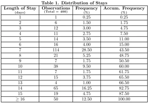
Table 1 lists the highest frequencies of length of stay. As expected, the highest frequency is 7 day stays, typically associated with tourists visiting on tour operator packages, with an in sample frequency of 28%. The combined frequency of 14-15 day stays is also quite high: about 20%. About half of the stays last no longer than 8 days.
<Insert Table 1 here>
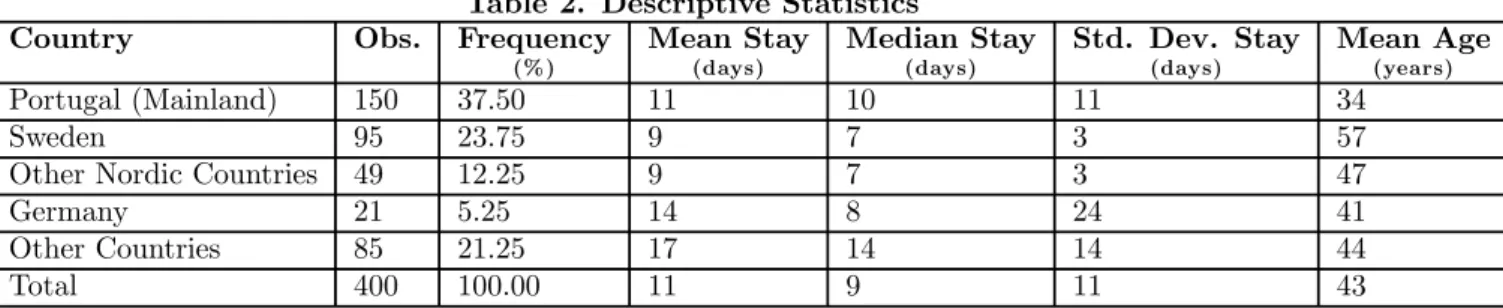
Table 2 contains additional descriptive statistics, for stays and age, by nationality.
<Insert Table 2 here>
Overall, mean stay is about 11 days, median stay is just 10 days while the standard deviation of stays is about 11 days, due to some quite long stays. The largest group of tourists in the sample are tourists from Mainland Portugal, who experience stays similar to those of the overall sample and are the youngest group. Tourists from the Nordic Countries are the second largest group in the sample and exhibit a mean stay of 9 days, a median stay of 7 days and a relatively low standard deviation of 3 days, as most of these tourists visit with either one or two week tour packages. German tourists experience, typically, longer stays than tourists from the Nordic Countries. In sum, there are interesting differences in length of stays across nationalities.
2.3
Survival Analysis: An Overview
Survival analysis is just another name for time to event analysis. The engineering sciences have contributed to the development of survival analysis which is called "reliability analysis" or "failure time analysis" in this field since the main focus is in modelling the time it takes for machines or electronic components to break down. Likewise, survival analysis has long been a cornerstone of biomedical research. The analysis of duration data comes fairly recently to the economics literature. Economists have recently applied the same body of techniques to strike duration, length of unemployment spells, time until business failure, and so on (for applications of survival analysis in economics, see, among others, Kieffer 1998; Lancaster 1990; Hosmer and Lemeshow 1999; Greene 2000). This section borrows heavily from Cleves, Gould and Gutierrez (2002). There are certain aspects of survival analysis data, such as censoring and non-normality, that generate great difficulty when trying to analyze the data using traditional statistical models such as multiple linear regression. The variable of interest in the analysis of duration is the length of time that elapses between the beginning of some event either until its end or until the measurement is taken, which may precede termination. Hence, it is sometimes the case that durations - the so-called spells - are censored, in the sense that the researcher does not observe the termination of the event.
This framework of analysis naturally lends itself to the study of length of stay, as one is interested in the determinants of the length of time that elapses between the tourist’s arrival on a given touristic destination and his departure. The data set employed in the present article was collected at airports from tourists who were departing from their trips. Hence, there is no censoring in the data since all interviewees reported their length of stay. Therefore, the discussion that follows assumes away censoring.
Spell length is, by construction, a non-negative variable. Let spell length be represented by a random variable T , with continuous probability distribution f (t), where t is a realization of T . The cumulative probability function F (t) reads:
F (t) = Z t
0 f (s)ds = Pr(T ≤ t)
(1)
It is usually the case that one is more interested in the probability that the spell is of length at least t, which is given by the survival function S(t):
S(t) = 1 − F (t) = Pr(T ≥ t) (2) The hazard rate, λ(t), in turn, answers the following question: Given that the spell has lasted until time t, what is the probability that it will end in the next short interval of time, ∆? More formally:
λ(t) = lim ∆−→0 Pr(t ≤ T ≤ t + ∆|T ≥ t) ∆ (3) = f (t) S(t)
Intuitively, the hazard rate is the rate at which spells are completed after duration t, given that they last at least until t. Armed with the hazard rate, one computes the survival function through backward integration:
S(t) = e−U0tλ(s)ds (4)
Two frequently used models for adjusting survival functions for the effects of covariates are the accelerated failure-time (AFT) model and the multiplicative or proportional hazards (PH) model. In the AFT model, the natural logarithm of the survival time, ln t, is expressed as a linear function of the (1 ∗ k) vector of time-invariant covariates x, yielding the linear model:
ln t = xβ + z (5)
where β is a (k ∗ 1) vector of regression coefficients to be estimated, and z is the error term with density f(). The distributional form of the error term determines the regression model.
In the proportional hazards model, the concomitant covariates have a multiplicative effect on the hazard function, satisfying, thus, a separability assumption:
λ(t, x) = λ0(t) exp(xβ) (6)
where λ0(t) is the baseline hazard function. Intuitively, the baseline hazard function λ0(t) summarizes the pattern of duration dependence and is common to all persons while λ = exp(xβ) is a non-negative function of covariates x, which scales the baseline hazard function common to all persons, controlling, hence, the effect of individual heterogeneity.
The PH property implies that absolute differences in x imply proportionate differences in the hazard rate at each t. For some t = t, and for two persons i and j with vectors of characteristics xi and xj:
λ(t, xi) λ(t, xj)
= exp(β´(xi− xj)) (7)
Hence, the proportional difference in the hazard rates does not depend on time, as long as the covariates are time independent, as in the present case. If, in addition, the two persons are identical in all matters except with respect to the kthcovariate, then a unit increase in the kthcovariate induces the following proportionate change in the hazard rates:
λ(t, xi) λ(t, xj)
= exp(βk) (8)
The above expression lends a natural interpretation to βk, namely, the log hazard ratio:
βk= ∂ log λ(t, x)/∂ log xk (9)
which is easily recognized as either a semi-elasticity or elasticity.
The baseline function h0(t) may be left unspecified, yielding the Cox’s PH model, or it may take a specific parametric distributional form, which, and assuming that the correct distributional form is chosen, leads to more efficient estimates.
The choice of a particular distribution matters since it conditions the slope of the hazard function. A particular distribution yields a particular hazard function, which may feature duration dependence, in the sense that the probability that termination of a stay occurs in the next short interval of time may depend on length of stay. Since there is scant or virtual none empirical evidence on the shape of the hazard function of lengths of stays, this paper takes an agnostic view and entertains the possibility of a myriad of shapes of the hazard function. Hence, the hazard function of stays is estimated under the following six alternative
distributions - exponential, Weibull, Gompertz, the three most popular PH models; generalized gamma, lognormal and log-logistic, the most widely employed AFT models - which altogether accommodate, ex ante, several possible shapes of the hazard function. It should be noted that this paper’s approach - of letting the data speak - allows to formally test some models against others, and, hence, select a model which is formally deemed as more appropriate.
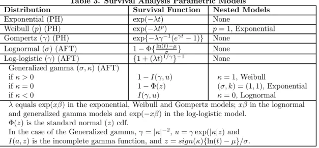
The exponential distribution yields a constant hazard rate λ0(t) = λ and hence is suitable to model length of stay when the probability of termination of a stay in the next short interval of time does not depend on the length of the stay. The Weibull distribution, in turn, is a generalization of the exponential distribution and is suitable for modelling data with monotone hazard rates that either increase or decrease exponentially with time. The corresponding baseline function is λ0(t) = pλtp−1 where p is an ancillary parameter to be estimated from the data. Note that when p = 1 the Weibull model collapses to the exponential model. The Gompertz distribution yields the baseline function λ0(t) = exp(γt), where γ is an ancillary parameter to be estimated from the data. Like the Weibull distribution, the Gompertz distribution is suitable for modelling data with monotone hazard rates that either increase or decrease exponentially over time. Unlike the PH models - namely the exponential, Weibull and Gompertz models -, the lognormal and log-logistic are two AFT models that tend to produce similar results and are indicated for data exhibiting nonmonotonic hazard rates, specifically initially increasing and then decreasing rates. Finally, the generalized gamma, another AFT model, yields an hazard function extremely flexible, allowing for a large number of possible shapes, including as special cases the Weibull, the exponential and the lognormal models. The generalized gamma model is, therefore, commonly used for evaluating and selecting an appropriate model for the data. Note that the lognormal model, the log-logistic model and the generalized gamma model are estimated in AFT form whilst the exponential model, the Weibull model and the Gompertz model are estimated in the PH form, and, therefore, the resulting regression coefficients β are not directly comparable.
<Insert Table 3 here>
Table 3 provides a summary of the main features of the six competing models (see Cleves, Gould and Gutierrez (2002) for more details on the distributions underlying the models presented in Table 3). The remainder of this section deals with model estimation and model selection.
2.4
Model Estimation and Model Selection
Model estimation is done via maximum likelihood, given the parametric nature of the six competing models. With respect to model selection, a reasonable question to ask is: "Given that we have several possible parametric models, how can we select one?". When parametric models are nested, the likelihood-ratio or Wald tests can be used to discriminate between them. This can certainly be done in the case of Weibull versus exponential, or gamma versus Weibull or lognormal. When models are not nested, however, these tests are inappropriate and the task of discriminating between models becomes more difficult. A common approach to this problem is to use the Akaike information criterion (AIC), which, in its essence, penalizes each log likelihood to reflect the number of parameters being estimated in a particular model and then
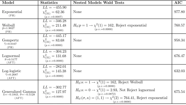
comparing them. The AIC is defined as AIC = −2(log likelihood) + 2(c + p + 1) where c is the number of model covariates and p is the number of model-specific ancillary parameters listed in Table 3. Although the best-fitting model is the one with largest log likelihood, the preferred model is the one with the smallest AIC value. Since the log likelihood obtained for any given parametric model depends on the set of covariates used, the set of covariates of interest is defined ex ante and then employed in the estimation of all the six competing models. Overall, 31 covariates were selected given the available data, on the one hand, and a reading of the literature, on the other, and are described at length in the next section, while the rest of this section focuses on model selection. Table 4 presents summary results of the log likelihood estimation, ancillary parameters, model discriminating Wald tests and AIC values.
<Insert Table 4 here>
The Weibull model dominates the exponential model in all criteria considered. The log likelihood obtained under the Weibull model is higher than the log likelihood obtained under the exponential model. A Wald test that p, the Weibull model ancillary parameter, is statistically equal to one - the case when the Weibull model collapses into the exponential model - is firmly rejected. In addition, the AIC value obtained under the Weibull model is lower than the AIC value obtained under the exponential model. Hence, the exponential model is not used elsewhere in this paper, since it is dominated by the Weibull model. Note that p has a point estimate of 1.9027, which is indicative of an upward sloping monotone hazard rate.
Like the Weibull model, the Gompertz model is suitable for modelling data with monotone hazard rates that either increase or decrease exponentially over time. Although the Weibull model cannot be formally tested against the Gompertz model, it should be noted that the Weibull model yields a higher log likelihood and a lower AIC value than the Gompertz model. Hence, the Weibull model is preferred to the Gompertz model and is the preferred PH model. Quite interestingly, the point estimate of γ, the ancillary parameter of the Gompertz model, is 0.0167, and, hence, the Gompertz’s model associated hazard rate displays a monotone and increasing hazard rate: the same result obtained under the Weibull model.
The log-logistic model produces the lowest AIC value of all the six models considered. The log-logistic model also produces the highest log-likelihood value among all the six competing models. The log-logistic model cannot be formally tested against the other models as it is a non-nested case. Hence, it is not possible to reject the idea that the log-logistic model produces the overall best fit to the data.
The lognormal model yields results similar to the log-logistic model, as expected. The generalized gamma model provides an array of discriminating Wald tests, as it nests the exponential model, the Weibull model and the lognormal model. The gamma model dominates the exponential model: not only does the generalized gamma model yields a lower AIC value and a higher log-likelihood but also the Wald test that (σ, κ) = (1, 1) produces a p-value of 0.0000. It is also the case that the generalized gamma model dominates the Weibull model. In fact, the generalized gamma model produces a lower AIC value than the Weibull model and, based on a discriminating Wald test κ = 1, the Weibull model is strongly rejected as a special case of the generalized gamma model. When the generalized gamma model is compared against the lognormal model, the picture that emerges is not so clear. The lognormal model corresponds to the generalized gamma model
in the special case κ = 0. The Wald test that κ = 0 yields a p-value of 0.0872, and hence it is not possible to reject the lognormal model at the 10% significance level. In addition, one can also argue in favor of the lognormal case since it produces a slightly lower AIC value than the generalized gamma model.
In conclusion, the Weibull model strictly dominates both the exponential and the Gompertz model, and is kept in the analysis since it is the preferred PH model. With respect to the AFT models considered, the lognormal model produces a slightly lower AIC value than the generalized gamma model and a discriminating Wald test on the generalized gamma model ancillary parameter κ fails to reject the lognormal model at the 10% significance level. Hence, there is some evidence that the lognormal model is preferred to the generalized gamma model. The log-logistic model produces not only the lowest AIC value but also the highest log likelihood of all six competing models, and cannot be formally tested against any other model as it is a non-nested model. Since the lognormal model and the log-logistic models produce remarkably similar results, the regression coefficients are reported only for the log-logistic model, to save on space.
2.5
Results
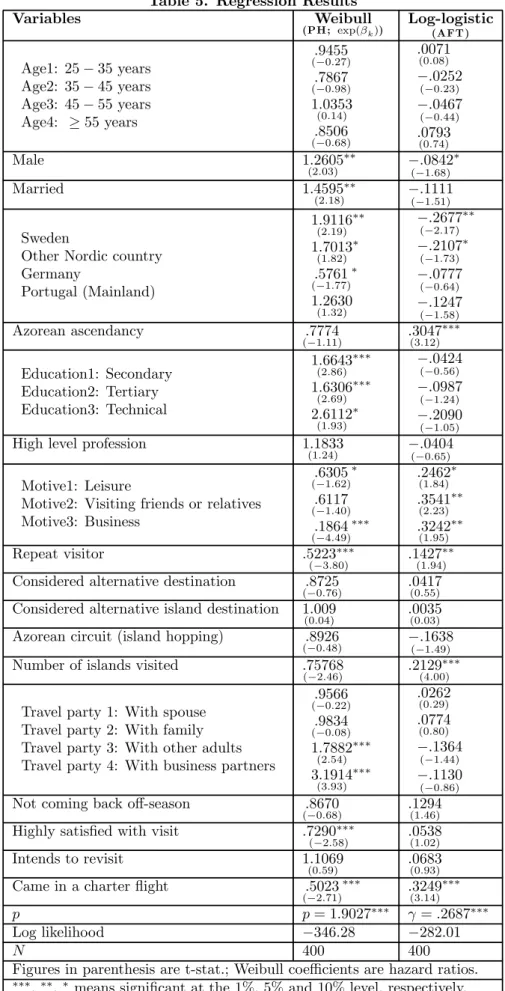
Table 5 reports the results obtained from the Weibull model - the preferred PH model - and the log-logistic model - the preferred AFT model. It should be noted that the coefficients are not directly comparable across models. The Weibull model is presented in PH form and the coefficients may be interpreted as a hazard ratio. Intuitively, and focusing on binary variables, the coefficients presented are of the form eβk and represent the
ratio between the hazard rate when the variable takes the value of 1 and the hazard rate when the variable takes the value of 0. Hence, a coefficient higher than one means that an increase in the variable leads to an increase in the hazard rate and, thus, to a lower expected duration. In turn, the log-logistic model is presented in AFT form and a negative coefficient is associated with shorter expected time to termination of a stay. Hence, and if one is interested in comparing the qualitative meaning of the coefficients across models, then coefficients higher (lower) than one in the Weibull model correspond to negative (positive) coefficients in the log-logistic model. Inspection of Table 5 reveals that, in fact, the Weibull model and the log-logistic model tend to produce the same results, at least at a qualitative level.
<Insert Table 5 here>
The age coefficients are not individually statistically significant in both models. As Alegre and Pou (2006) suggest, this may owe to the inclusion of other covariates closely related with age. However, and given that the excluded class is less than 25 years, the results suggest that older tourists tend to stay longer, a result in line with Alegre and Pou.
Male tourists tend to experience shorter stays, just like married tourists. These results obtain for both the Weibull model and the log-logistic model. However, they are only significant in the case of the Weibull model.
Tourists from the Nordic Countries, Sweden included, experience shorter stays, under both models. These results are statistically significant and have important policy implications given the strategical importance of these markets in the overall policy context. In turn, German tourists exhibit longer stays. However, this
result for German tourists is only marginally statistically significant in the Weibull model and not statistically significant in the log-logistic model. Tourists from Mainland Portugal, who constitute the largest group in the sample, exhibit shorter stays, under both models; a result with no statistical significance. Overall, the regression coefficients on nationalities do not follow any clear pattern, at least not according to the physical distance between the tourist’s place of origin and destination. In fact, ex ante one would imagine that tourists who live far away would experience longer stays, to make up for the increased overall travel cost. Hence, while it is indeed the case that tourists who live close to the Azores, such as tourists from Portugal Mainland, do tend to experience shorter stays than tourists who live farther away as, say, tourists from the Nordic countries, when one controls for sociodemographic profiles and trip attributes, this pattern becomes less blunt. This is indeed the present case. In particular, it is found that the binary variable charter that equals 1 if the tourist took a (direct) charter flight (and 0 otherwise) significantly increases the length of stay. Considering that virtually all tourists from the Nordic Countries took charter flights, it becomes less of a paradox that having a nationality from the Nordic Countries is associated with shorter length of stays. The reverse could be said about tourists from Mainland Portugal. This remark highlights the importance of controlling for a significant number of covariates.
Azorean ascendancy is a binary variable that equals 1 in case the tourist claims to have some sort of Azorean ascendancy. The Azorean diaspore far outnumber the current Azorean population and there are many Azorean descendents, typically residing in North America, who visit the Azores. It is found, in both models, that having an Azorean ascendancy reduces expected time to termination of stays, a result highly statistically significant under the log-logistic model.
With respect to the education variables, it should be noted that the excluded class is other education, an education class associated with a lesser degree of education. Hence, it follows that both models suggest that higher levels of education are associated with shorter stays, albeit with statistical significance only in the Weibull model.
High level profession is a binary variable that takes the value of 1 for professions associated with high incomes and high social status. In this sense, high level profession proxies top incomes. A first group of 50 tourists were interviewed in a first stage of the field work in order to validate the questionnaire. From this validation exercise, it followed that not all tourists were willing to report directly their income, and, hence, such proxy for income, based on current professional status, was built in the questionnaire. In both models, a high level profession is associated with shorter expected duration of stays; a result with no statistical significance.
Travel motive was divided into four classes: leisure; visiting friends or relatives; business and, the excluded class, other motives (which includes, for instance, religious festivities). It is found that, compared to the excluded class, all travel motives explicitly considered increase expected duration of stays, a result with high statistical significance in the log-logistic model. As Seaton and Palmer (1997) suggest, tourists visiting friends or relatives tend to exhibit longer stays if they are international tourists, as it is generally the case in the Azores.
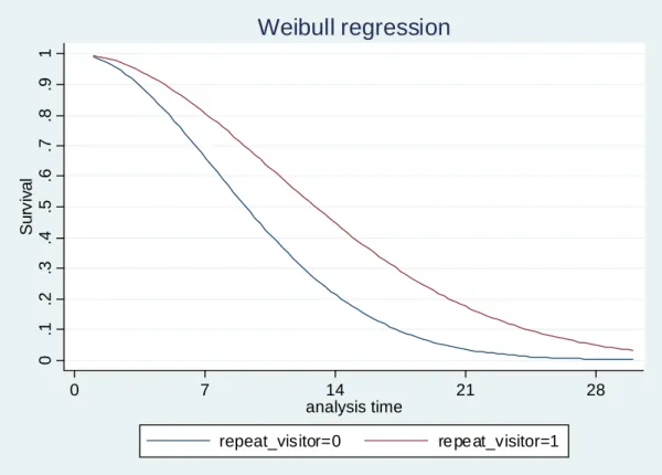
Repeat visitor is a binary variable that takes the value of 1 if the tourist visited the Azores at least once in the past, and 0 otherwise. Quite interestingly, in both models it is found that repeat visitors stay for longer periods. In fact, everything else the same, being a repeat visitor reduces the hazard rate to half (0.5223) in the Weibull model. Repeat visitor behavior has aroused interest in the recent years (see, among others, Oppermann 1997; Kozak 2001 and Lehto, O’Leary and Morrison 2004), has its relationship with future visiting behavior (destination loyalty) and word-of-mouth recommendation carries important policy and marketing implications. While such analysis is beyond the scope of this paper, it is interesting to note the strikingly different expected on-site time spent by repeaters from first-timers, as Figure 1 documents. Figure 1 plots two survival functions, one for repeat visitors and one for first-time visitors. The survival function for repeat visitors is shifted to the right, which means that repeat visitors are associated with a higher probability of experiencing a stay of at least a given duration. For instance, the probability that repeaters stay for at least 14 days is about 45%, more than double the analogous probability for first-timers: about 20%.
<Insert Figure 1 here>
Considered alternative destination and considered alternative island destination are two dummy variables that characterize the destination decision process. However, both variables are not statistically significant in both models.
There are nine islands in the Azores. However, most tourists visit only one island: São Miguel. Azorean circuit is a binary variable that takes the value of 1 in case the tourist visits more than one island. In both models, engaging in island hopping does not influence expected length of stay, at least in a statistical sense. Number of islands considered, in turn, is a continuous variable ranging from 1 to 9, since there are nine islands in the Azores. Hence, it can be argued that number of islands embeds richer information then Azorean circuit, since the former is continuous while the latter is binary. While in the Weibull model the number of islands visited is not statistically significant at the conventional levels, in the log-logistic model an increase in the number of islands visited leads to an increase in the expected length of stay, as expected. The questionnaire was carried out in the Summer. To gauge the degree of tourists’ satisfaction with their experience in the Azores, it was asked if tourists would consider visiting the Azores off-season (when the weather is arguably not so pleasant). Not coming back off season flags the tourists who answered no. In both models, not coming back off season has no statistical significance. Highly satisfied with visit is a binary variable that directly captures overall tourists’ satisfaction with respect their experience. While in the log-logistic model being highly satisfied with the visit has no statistical significance, in the Weibull model being highly satisfied with the visit leads to longer expected length of stays. This result may owe to the fact that highly satisfied tourists prolonged their stays or tourists who report to be highly satisfied are those who were indeed more likely to enjoy their visit and hence planned longer stays from the onset of their visits.
Perhaps not surprisingly, taking a charter flight causes longer expected stays. This result has important policy implications as charter flights are subsidized by the local government.
3
Conclusion
One of the most important decisions made by tourists before or while visiting a given destination concerns their length of stay. In fact, length of stay most likely conditions overall tourist expenditure and stress imposed on local resources, just to name a few of the implications of varying lengths of stays. However, and as Alegre and Pou (2006) document, despite the rich literature on tourism demand, very few studies have resorted to microeconometric models in order to shed light on the determinants of length of stay. This paper estimated a number of alternative microeconometric parametric survival analysis models to learn the determinants of length of stay, in a novel way in the tourism demand literature. The results are statistically significant and economically important. Quite interestingly, a large number of covariates, pertaining to detailed individual sociodemographic profiles and actual trip experiences of the representative tourists interviewed, were considered in the regressions in order to control for heterogeneous individual behavior. Concomitantly, the richness of the information embedded in the covariates used allows the design of effective marketing policies, in the sense that the regression results allow one to estimate, for a given synthesized, policy relevant individual or target group, not only mean or median expected stays, but also the probability that stays exceed a given threshold. Hence, policymakers and private operators may benefit from such tools that uncover individual sociodemographic profiles and trip attributes that promote longer stays and act or advertise accordingly. Among the several results found, it can be argued that being a repeat visitor and taking charter flights are important criteria to identify tourists who are likely to experience longer stays. In fact, it is shown that repeaters face a 45% probability of experiencing a stay of at least 14 days, which is more than double the analogous probability for first-timers of 20%. Thus, future research should characterize such groups and their economic and activity involvement. Taking a (direct) charter flights also plays a highly statistically significant role in determining length of stay. In particular, taking a charter flight decreases the hazard rate to half, and, hence, leads to longer expected stays. This result is very important as the Azorean government, in its quest to promote air connections to the Azores, subsidizes charter flights, and, must, therefore, assess the socioeconomic implications of such subsidies. Apparently, such policy is successful in terms of promoting longer stays. This is true regardless of nationalities, which were controlled for in the regressions. A higher degree of education is associated with shorter expected stays. It would be interesting to investigate if this result follows from better educated tourists face more stringent time constraints or are purely due to differences in preferences across education levels. Visiting more islands leads to an increase in the expected length of stay. This result suggests that there is no crowding-out behavior from the part of tourists, in the sense that tourists do not trade a larger number of islands visited for a shorter visit per island, keeping, hence, overall length of stay constant. In the contrary: tourists are willing to visit more islands at the expense of longer stays. Thus, policymakers ought to arouse tourists’ interest for visiting a large number of islands. For instance, what role does inter-island mobility play? By the same token, it is important to note that reporting a high degree satisfaction has a statistically significant positive impact on expected stays. Hence, understanding what causes a high overall degree of satisfaction is also an important future research topic.
References
[1] Alegre, J., and L. Pou
2006 The Length of Stay in the Demand for Tourism. Tourism Management 27: 1343-1355.
[2] Bargeman, B., and van der Poel
2006 The Role of Routines in the Decision Making Process of Dutch Vacationers. Tourism Manage-ment 27: 707—720.
[3] Cleves, M., Gould, W., and R. Gutierrez
2002 An Introduction to Survival Analysis Using Stata. College Station Texas: Stata Press.
[4] Crouch, G.
1994 A Meta-Analysis of Tourism Demand. Annals of Tourism Research 22: 103-118.
[5] Crouch, G., and I. Louviere
2000 A Review of Choice Modelling Research in Tourism, Hospitality, and Leisure. Tourism Analysis 5: 97-104.
[6] Davies, B., and J. Mangan
1992 Family Expenditure on Hotels and Holidays. Annals of Tourism Research 19: 691-699.
[7] Decrop, A., and D. Snelders
2004 Planning the Summer Vacation: An Adaptable and Opportunistic Process. Annals of Tourism Research 31: 1008-1030.
[8] Fleischer, A., and A. Pizam
2002 Tourism Constraints Among Israeli Seniors. Annals of Tourism Research 29: 106-123.
[9] Gokovali, U., Bahar, O., and M. Kozak
2007 Determinants of Length of Stay: A Practical Use of Survival Analysis. Tourism Management in press.
[10] Green, W.
2000 Econometric Analysis. New Jersey: Prentice Hall.
[11] Hill, M., and A. Hill
2002 Research with Surveys. Lisbon: Sílabo.
[12] Hosmer, D., and S. Lemeshow
[13] Kiefer, N.
1988 Economic Duration and Hazard Functions. Journal of Economic Literature 26: 646—667.
[14] Kozak, M.
2001 Repeaters’ Behavior at Two Distinct Destinations. Annals of Tourism Research 28: 785-808.
[15] Kozak, M.
2004 Destination Benchmarking: Concepts, Practices and Operations. Oxon Cab: CAB Interna-tional.
[16] Lancaster, T.
1990 The Econometric Analysis of Transition Data. Cambridge: Cambridge University Press.
[17] Lehto, X., O’Leary, J., and A. Morrison
2004 The Effect of Prior Experience on Vacation Behaviour. Annals of Tourism Research 31: 801-818.
[18] Legoherel, P.
1998 Toward a Market Segmentation of the Tourism Trade: Expenditure Levels and Consumer Behavior Instability. Journal of Travel and Tourism Marketing 7: 19-39.
[19] Lim, C.
1997 An Econometric Classification and Review of International Tourism Demand Models. Tourism Economics 3: 69-81.
[20] Mok, C., and T. Iverson
2000 Expenditure-Based Segmentation: Taiwanese Tourists to Guam. Tourism Management 21: 299-305.
[21] Oppermann, M.
1995 Travel Life Cycle. Annals of Tourism Research 22: 535-552.
[22] Oppermann, M.
1997 First-time and Repeat Visitors to New Zealand. Tourism Management 18: 177-181.
[23] Saarinen, J.
2006 Traditions of Sustainability in Tourism Studies. Annals of Tourism Research 33: 1121-1140.
[24] Seaton. A., and C. Palmer
1997 Understanding VFR Tourism Behavior: The First Five Years of the United Kingdom Tourism Survey. Tourism Management 18: 345-355.
[25] Song, H., and S. Witt
2000 Tourism Demand Modelling and Forecasting: Modern Econometric Approaches. Oxford: Per-garmon.
[26] Sung, H., Morrison, A., Hong, G., and J. O’Leary
2001 The Effects of Household and Trip Characteristics on Trip Types: A Consumer Behavioural Approach for Segmenting the US Domestic Leisure Travel Market. Journal of Hospitality & Tourism Research 25: 46-68.
[27] Witt, S., and C. Witt
1995 Forecasting Tourism Demand: A Review of Empirical Research. International Journal of Fore-casting 11: 447-475.
Table 1. Distribution of Stays Length of Stay
(days)
Observations
(Total = 400) Frequency(% ) Accum. Frequency(% )
1 1 0.25 0.25 2 6 1.50 1.75 3 12 3.00 4.75 4 11 2.75 7.50 5 14 3.50 11.00 6 16 4.00 15.00 7 114 28.50 43.50 8 21 5.25 48.75 9 7 1.75 50.50 10 38 9.50 60.00 11 7 1.75 61.75 12 15 3.75 65.50 13 4 1.00 66.50 14 65 16.25 82.75 15 19 4.75 87.50 ≥ 16 50 12.50 100.00
Table 2. Descriptive Statistics Country Obs. Frequency
(% ) Mean Stay (days) Median Stay (days) Std. Dev. Stay (days) Mean Age (years) Portugal (Mainland) 150 37.50 11 10 11 34 Sweden 95 23.75 9 7 3 57
Other Nordic Countries 49 12.25 9 7 3 47
Germany 21 5.25 14 8 24 41
Other Countries 85 21.25 17 14 14 44
Table 3. Survival Analysis Parametric Models Distribution Survival Function Nested Models Exponential (PH) exp(−λt) None
Weibull (p) (PH) exp(−λtp) p = 1, Exponential Gompertz (γ) (PH) exp{−λγ−1(eγt− 1)} None
Lognormal (σ) (AFT) 1 − Φ{ln(t)σ−µ} None Log-logistic (γ) (AFT) {1 + (λt)1/γ}−1 None
Generalized gamma (σ, κ) (AFT) if κ > 0 if κ = 0 if κ < 0 1 − I(γ, u) 1 − Φ(z) I(γ, u) κ = 1, Weibull (σ, k) = (1, 1), Exponential κ = 0, Lognormal
λ equals exp(xβ) in the exponential, Weibull and Gompertz models; xβ in the lognormal and generalized gamma models and exp(−xβ) in the log-logistic model.
Φ(z) is the standard normal (z) cdf.
In the case of the Generalized gamma, γ = |κ|−2, u = γ exp(|κ|z) and I(a, z) is the incomplete gamma function, and z = sign(κ){ln(t) − µ}/σ.
Table 4. Model Selection
Model Statistics Nested Models Wald Tests AIC
Exponential (PH) LL = −455.90 χ2(31)= 62.36 (p.v.=0.0007) None 977.80 Weibull e p=1.9027 (PH) LL = −346.28 χ2(31)= 211.48 (p.v.=0.0000) H0:p = 1 → χ2(1) = 162 (p.v.=0.0000) , Reject exponential 760.57 Gompertz e γ=0.0167 (PH) LL = −445.17 χ2 (31)= 83.68 (p.v.=0.0000) None 958.34 Lognormal e σ=0.5177 (AFT) LL = −304.23 χ2(31)= 131.68 (p.v.=0.0000) None 676.47 Log-logistic e γ=0.2687 (AFT) LL = −282.01 χ2 (31)= 145.38 (p.v.=0.0000) None 632.03 Generalized Gamma e κ=−0.1843, eσ=−0.5128 (AFT) LL = −302.77 χ2 (31)= 127.97 (p.v.=0.0000) H0:κ = 1 → χ2(1) = 162 (p.v.=0.0000) , Reject Weibull H0:κ = 0 → χ2(1) = 2.93 (p.v.=0.0872)
, Not Reject lognormal
H0:(σ, κ) = (1, 1) → χ2(2) = 764.41 (p.v.=0.0000)
, Reject exponential
Table 5. Regression Results Variables Weibull (PH ; exp(βk)) Log-logistic (AFT ) Age1: 25 − 35 years Age2: 35 − 45 years Age3: 45 − 55 years Age4: ≥ 55 years .9455 (−0.27) .7867 (−0.98) 1.0353 (0.14) .8506 (−0.68) .0071 (0.08) −.0252 (−0.23) −.0467 (−0.44) .0793 (0.74) Male 1.2605 (2.03) ∗∗ −.0842 (−1.68) ∗ Married 1.4595∗∗ (2.18) −.1111(−1.51) Sweden
Other Nordic country Germany Portugal (Mainland) 1.9116 (2.19) ∗∗ 1.7013 (1.82) ∗ .5761 (−1.77) ∗ 1.2630 (1.32) −.2677 (−2.17) ∗∗ −.2107 (−1.73) ∗ −.0777 (−0.64) −.1247 (−1.58) Azorean ascendancy .7774 (−1.11) .3047(3.12) ∗∗∗ Education1: Secondary Education2: Tertiary Education3: Technical 1.6643 (2.86) ∗∗∗ 1.6306 (2.69) ∗∗∗ 2.6112 (1.93) ∗ −.0424 (−0.56) −.0987 (−1.24) −.2090 (−1.05) High level profession 1.1833
(1.24) −.0404(−0.65) Motive1: Leisure
Motive2: Visiting friends or relatives Motive3: Business .6305 (−1.62) ∗ .6117 (−1.40) .1864 (−4.49) ∗∗∗ .2462 (1.84) ∗ .3541 (2.23) ∗∗ .3242 (1.95) ∗∗ Repeat visitor .5223∗∗∗ (−3.80) .1427 ∗∗ (1.94) Considered alternative destination .8725
(−0.76) .0417(0.55) Considered alternative island destination 1.009
(0.04) .0035(0.03) Azorean circuit (island hopping) .8926
(−0.48) −.1638(−1.49) Number of islands visited .75768
(−2.46) .2129 ∗∗∗ (4.00)
Travel party 1: With spouse Travel party 2: With family Travel party 3: With other adults Travel party 4: With business partners
.9566 (−0.22) .9834 (−0.08) 1.7882 (2.54) ∗∗∗ 3.1914 (3.93) ∗∗∗ .0262 (0.29) .0774 (0.80) −.1364 (−1.44) −.1130 (−0.86) Not coming back off-season .8670
(−0.68) .1294(1.46) Highly satisfied with visit .7290∗∗∗
(−2.58) .0538(1.02) Intends to revisit 1.1069
(0.59) .0683(0.93) Came in a charter flight .5023
(−2.71) ∗∗∗ .3249 (3.14) ∗∗∗ p p = 1.9027∗∗∗ γ = .2687∗∗∗ Log likelihood −346.28 −282.01 N 400 400
Figures in parenthesis are t-stat.; Weibull coefficients are hazard ratios. ∗∗∗,∗∗,∗ means significant at the 1%, 5% and 10% level, respectively.
0 .1 .2 .3 .4 .5 .6 .7 .8 .9 1 Su rv iv a l 0 7 14 21 28 analysis time repeat_visitor=0 repeat_visitor=1