Testing the link specification in binary choice models. A semiparametric approach.

UNIVERSITE CATHOLIQUE DE LOUVAIN

FACULTE DES SCIENCES ECONOMIQUES, SOCIALES ET POLITIQUES

Nouvelle serie-N°259

- - I. S. E. <e;i, - - .

:!".

~~ulioteca

::{Jlf:?.(P.

43930

HD3o.

23.

74--b

19"1'S"

TESTING THE LINK SPECIFICATION

IN BINARY CHOICE MODELS.

A SEMIPARAMETRIC APPROACH.

Isabel PROEN<;A

CIA CO Louvain-la-Neuve

....

j)A

GQv-cvR~

111CLA A,o G-f\P>\J v't.

~0\?1'\...

E. (L

E C..O NCi (LC{.!) CoN C'C...-J> 'C J) Pr ( \ . lA '-.l N C"-k

f'L

-5

"C. 9 A 3> t- '-;z:_c r-JL.l.P.> :;) C...

~~

1'3C. A r-=\\<7 8

v-C:.:. .\

pc.

-r:('l

s.

~'1\S..-u s~

l'l< (l....Lu (L. Dl::.. E co

NQ~t.-u:::,

c

G-<e

s;--;-~~

Ao

A~

l'l/CCJv '3)c.

vcc_c_.r·t.£..\b

-u.c

~.

;;L<t; 3

t~'3,.

.D<i- 2).

D~

::J'-' N rt-o. (:; S\A

o

(3 N="> NA-b (?oy<c_ f"lA.-

S~IL

Cl'z.

~to

;>,rz_-:

:.>A Du p J -.-a -'L ₁ Cf.J'I\IJ~~ '<-~

-.S, ~ 1'L- ~.X. f n .. '~c--~ ~ a (L'<:-.) .> Pd .. -v A D/1 5 ~.) DeS Pa-' -.:::-~c.,~ priT' '::\-G 7 1 :!)D coDCCi<l D<> z;iCrLe.ZTl> p,0\b!\- ( D

£:..C.Jl~

-ro-

L'C:t:

1\J,"

3

l~,;-

I 'Dt.

A.4.

'Af\_~t1Uf ) • L "C) GG P-1 ., ' _I

(}Oo

/,7\J]/W_~2/

~~~l:Xr

~

~W/

-E~

₄

W / )

cU_

£(u~

~L-cckce~

Clf·

~

~~

RLotdcr~

cf\

ch

~e_ ~cci>1

ih_

tu:_

ra<-

ck_

~~~~~~~~

~

~-&::_

dA-

Jf

~

A4~

'i> _

List of Figures iv

List of Tables vii

Acknowledgments 1

Introduction 4

1 Parametric Binary Model 7

1.1 Introduction 0 0 0 0 0 0 0 7

1.2 The Utility Function Approach 9

1.3 The Latent Variable Model 12

1.4 Nonlinear Least Squares 14

1.5 Parametric Models 0 16

1.6 Multinomial Models 19

1.601 Unordered Multinomial Models 20

1.602 Ordered Models 22

1.603 Sequential Models 22

1.7 Applications 0 23

1.8 An Example 0 26

ii CONTENTS •'

'I

2.1 Introduction . 33

2.2 The model .. 34

2.3 Semiparametric estimation of the SIM 35 2.3.1 WADE Estimator • • • 0 • • • 38

2.3.2 Maximum Quasi-Likelihood Estimator 39 2.3.3 Semiparametric Least Squares Estimator 41

2.4 The Example Revisited 41

2.5 Confidence Bands . 43 2.6 Applications . . . . 49 2.7 Concluding Remarks 54 3 The HH-test 59 3.1 Introduction . 59 3.1.1 The Problem 61

3.1.2 Specification Tests for Binary Choice Models 62

3.2 The HH-test Statistic

...

65

3.2.1 Known Index Function . 66

3.2.2 The HH-test as a CM test. 67

3.2.3 The HH-statistic Under the Alternative 69

3.2.4 Estimated Index Function 69

3.3 Applications . . . 71

3.4 Concluding Remarks 76

4 Finite Sample Properties of the HH-test 77 4.1 Introduction . . . 77 4.2 Description of the Experiment Design 79

4.3 The Role of the Corrections . . 80

5

4.3.2 Results . . . . 4.4 The Effect of Estimating the Index Function 4.5 Results on Empirical Size and Power

4.6 Concluding Remarks . . .

Bootstrapping the HH-test 5.1 Introduction . . . . 5.2 The bootstrap approach 5.3 Monte Carlo study 5.4 Applications . . . . 5.5 Concluding Remarks

6 A modified HH-test 6.1 The modified statistic

6.2 Effect of Estimating the Index Function 6.3 Alternative Bias Correction . . . . 6.4 Performance of the Modified Statistic 6.5 Comparison between MHH and BHH tests .

6.6 Concluding Remarks .

7 Empirical Applications 7.1 Introduction . . . .

7.2 Modelling Unemployment after Apprenticeship 7.2.1 The Data . . . .

7.2.2 The Parametric Fit. 7.2.3 The Semiparametric Fit

7.2.4 Testing the Adequacy of the Logit Link 7.3 The Credit-Scoring problem .

7.3.1 The Data . . . . 82 85 96 105 107 107 108

111

116 117 119 120 123 125 127 137 141 143 143 144 144 146 148 149 153 153

iv

7.3.2 The Parametric Fit . . . 7.3.3 The Semiparametric Fit

7 .3.4 Testing the Adequacy of the Logit Link

7.4 Concluding Remarks Conclusions A Proof of Theorem 6.1 B XploRe Procedures Bibliography CONTENTS

.

~ •'

154

155

157

160

161 165 169 179

1.1 Fit of the probability of choice of car for travel to work 8

1.2 Credit-Scoring curve • • • • • 0 9

1.3 Probit, Logit and CLL models 17

1.4 Fit of the probability of choice of car for travel to work 24

1.5 Credit-Scoring curve • • • • 0 25

1.6 Binary choice models:logit fit 28

1.7 Binary choice models:logit fit - index normalized 29 1.8 Binary choice models:an example . . . 30

2.1 Probability of choice of car for travel to work 37 2.2 Credit-Scoring curve 0 0 • • • • • • 0 0 0 0 38

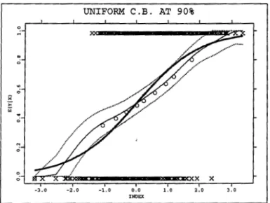
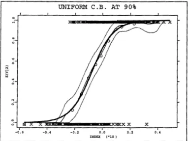
2.3 Uniform confidence bands - parametric fit. Correct specification 46 2.4 Uniform confidence bands - parametric fit. Misspecified link . . 47 2.5 Uniform confidence bands- semiparametric fit. Correct

specifi-cation . . . 49 2.6 Uniform confidence bands- semiparametric fit. Misspecified link. 50 2.7 Fit of the probability of choice of car for travel to work 52 2.8 Credit-Scoring curve . . . 53 2.9 Uniform confidence bands for the Transportation Mode Choice. 54 2.10 Uniform confidence bands for the Credit-Scoring. . . 55

List of Tables

1.1 Estimates for the mode-choice to travel data . 24 1.2 Estimates for the credit-scoring data 25 1.3 Results of the logit fit • • • • 0 0 • • 31

2.1 Results of the Parametric and Semi parametric fits 42 2.2 Estimates for the mode-choice to travel data . 52 2.3 Estimates for the credit-scoring data . . . . 53

3.1 HH-test for the mode-choice to travel data 71 3.2 HH-test for the credit-scoring data . . . 73

4.1 Percentiles, mean and standard deviation of the HH-test statis-tic under correct specification. . . 93 4.2 Percentiles, mean and standard deviation of the HH-test

statis-tic under misspecification • 0 0 0 0 0 0 • 0 • 0 • 0 • • • 0 • • • 94

4.3 Percentages of rejections of the HH-test for 100 observations 101 4.4 Percentages of rejections of the HH-test for 200 observations 102 4.5 Percentages of rejections of the HH-test for 400 observations 103 4.6 Percentages of rejections of the HH-test for 1000 observations 104

5.1 Rate of rejections of the classic and bootstrapped tests . . . 114 5.2 BHH-test for the mode-choice to travel and credit-scoring data 116

6.1 Percentiles, mean and standard deviation of the MHH-test statis-tic under correct specification . . . 135 6.2 Percentages of rejections of the MHH-test for 100 observations 136 6.3 Percentages of rejections of the MHH-test for 200 observations 137 6.4 Percentages of rejections of the MHH-test for 400 observations 138 6.5 Percentages of rejections of the MHH-test for 100 observations 139 6.6 Percentages of rejections of the MHH-test for 100 observations 140

7.1 Explanatory Variables for the unemployment after apprentice-ship data. . . 145 7.2 Results of the Logit Fit - Full Model. Unemployment data. 147 7.3 Results of the logit fit- restricted model. Unemployment data. 147 7.4 Results of the Semiparametric fit- restricted model.

Unemploy-ment data . . . 148 7.5 Results for the HH-test and Modified HH-test. Unemployment

data. . . 151 7.6 Results for the HH-test and bootstrap critical values.

Unem-ployment data. . . 152 7.7 Explanatory Variables for the credit-scoring data. 154 7.8 Results of the Logit Fit - Full Model. Credit-scoring data. 155 7.9 Results of the logit fit -restricted model. Credit-scoring data . 156 7.10 Results of the Semiparametric fit - restricted model.

Credit-scoring data. . . 157 7.11 Results for the HH-test and bootstrap critical values.

Credit-scoring data. . . 160

Acknowledgments

I am deeply grateful to my parents for their care, encouragement and example which have enlightened me and given a meaning for the effort I had to devote to accomplish this work.

I am special grateful to my dear friends Isabel, Carlos and Joao Luis who have convinced me and gave me the courage to start this adventure.

I am strongly indebted to Professor Bento Murteira who guided my research in Portugal for all his care and support. His dedication to work, honesty and generosity are for me a permanent inspiration.

This thesis would not have been possible without the commitment of my advisor Wolfgang Hardie. I have learned from him not only about econometrics and research but also about life. He has taught me to be ambitious, self confi-dent in improving my capacities and to fight for what I believe. I am thankful for all his support and the opportunities he gave me.

I feel a deep gratitude to my co-author Christian Ritter. His determination and guidance have encourage me to proceed the work. Without him chapter 6 would not have been possible. I am thankful to my other co-author Axel Werwartz. To work together with them was a pleasure and a rich experience.

I have to acknowledge the members of the jury ofthis thesis, Joel Horowitz, Luc Bawens, Leopold Simar and Alois Kneip for their valuable comments and suggestions that much have improved this dissertation. All the errors are my responsibility. A special thank is due to Luc Bawens whose careful notes on the original text have being a precious help in its revision.

I am thankful to my friend Joao Santos Silva who read the manuscript and gave me interesting suggestions. For instances, he has pointed me out the work of Ruud.

I am grateful to all professors and visitors of CORE and Institut de

tique with whom I have discussed my work and received valuable comments. I have to mention among them Alexander Tsybakov, Alois Kneip, Birgit Grund, Enno Mammen, Hidehiko Ichimura, Joel Horowitz, Jorg Polzehl, Luc Bawens, Michel Delecroix, Peter Hall and Rodney Wolff.

While I was doing this work I have been invited by some researcher cen-ters where I had very fruitful discussions and enjoyed my stay. Wolfgang Hardie has invited me several times to visit the Institut fiir Statistik und Okonometrie, Humboldt-Universitat zu Berlin, Juan Rodriguez has invited me to the Economics department of the Universidade de Bilbao, Wenceslao Gonzalez-Manteiga has invited me to the Mathematics department of the Uni-versidade de Santiago de Compostela, Michel Delecroix has invited me to EN-SAE, Paris and Emmanuel Jolivet has invited me to INRA, Paris. To them and the respective researcher centers all my gratitude.

I am grateful to Joel Horowitz and to Ludwig Fahrmeir who allowed me to use the data sets about respectively mode choice to travel on the way to work and credit-scoring. I thank Marlene Miiler who was helpful on providing me these data sets. I am grateful too to Jean-Marie Rolin who allowed me to use the other credit-scoring data set referring to the Flemish region of Belgium. I thank also Cecile Denis in her help on arranging that data set. Still about data, I have to remark the great work of Axel Werwatz on preparing the data set about unemployment after apprenticeship. All my thanks.

I have to acknowledge the way I was welcomed at CORE and Institut de Statistique, their cooperative staff, and the stimulating scientific environment that made possible the research behind this thesis.

I owe special thanks to Berwin Turlach and Sigbert Klinke for their ex-pert help with computers and computation problems. Berwin gave me also a precious help with LateX. I wish to thank too Valentin Patilea and Christian Weiner for the fruitful discussions and fine insights.

I have to thank the financial support I had that made possible the achieve-ment of this work. Namely, the grant I had from JNICT (Junta Nacional de Investigac;ao Cientifica) and the grant provided by FDS to pursuit the develop-ment of the project "Enseignedevelop-ment da la Statistique sur ordinateur personnel". I have to thank also the support of the Insituto Superior de Economia e Gestao (ISEG), Universidade Tecnica de Lisboa which has released me from my teach-ing duties durteach-ing my stay at Louvain-La-Neuve.

I am grateful to Heraklis Polemarchakis and Jayasry Dutta for their gener-ousity and the care they show to the Ph. D. students.

f'

-ACKNOWLEDGMENTS 3

During my stay at Louvain-La-Neuve I had the fortune to meet a lot of nice people with whom I have shared pleasant moments, namely my colleagues at CORE and Institut de Statistique. I am thankful for they made my life enjoyable.

Finally, to my friends that made this work possible for being at my side in the bad moments and gave me the joy of their companionship at Louvain-La-Neuve I wish to express all my deep gratitude: Isabel, Cinzia, Marlene, Juan, Maria Joao, Pedro, Miguel and Macarena, Fatima, Abdur, Manuel, Fernando, Irene, Sigbert, Marco and Marcela, Marga, Arantza, Viviane, and specially Berwin. You will remain all in my heart.

This thesis will be centered on the field of microeconometrics by dealing with models that describe the behavior of individual decision making units. Mi-croeconomic theory provides a rich framework to analyze and understand the motive of individual decision units. Econometrics has the task to quantify the structure describing individual decision actions for a given population using data that are real measurements characterizing the individuals of this pop-ulation. There is surely an important interaction between both disciplines. Econometrics needs the knowledge of microeconomics to specify the models quantifying the individual behavior. However, econometrics results are impor-tant to economic theory to validate the assumptions and hypotheses postulated or to guide the specification of new hypotheses.

The models discussed in this thesis belong to the class of qualitative choice models (also known as discrete choice models). These models specify the prob-ability that a given individual will choose a particular alternative from a well specified set of alternatives. Probit, logit, conditional probit and multinomial logit are examples of such models. There are many applications in economics concerning qualitative choice models including choice of housing (choice be-tween buying a certain good or a substitute), transportation (choice bebe-tween individual or public transportation on the way to work) and labor market (choice of a worker whether to take a job offer or not). For example, Train (1986), investigates household vehicle demand. Some of his models estimate the probability of a household to own one, two or more automobiles, others estimate the probability of a household to choose one vehicle amongst a set of classes of different vehicles (foreign vs domestic, or choice between auto-mobiles of different sizes are examples). Horowitz (1993) presents a model to estimate the probability of choice between automobile and transit for travel to work. van Soest (1992) fits a neoclassical structural model oflabor supply (or choice between labor and leisure) of both spouses. Berridge (1993) models job security.

INTRODUCTION

Parametric models like the probit and the logit are very popular because they are computationally tractable and easy to interpret. They rely on the specification of a certain distribution (respectively the standard normal or the logistic) for the probabilities of choice and the homoscedasticity (that is equal variance for all individuals) but real situations can be more complex. That is, heterogeneity among the preferences of the decision makers is likely to be present or the probabilistic structure of the model may not follow exactly the probit or logit classic specification.

An alternative to parametric models relying on much less assumptions are semiparametric models like the so-called single index. Briefly, these models consist in an unknown transformation of a linear function with an unknown finite number of parameters while parametric models like the probit or logit consist in a known transformation of the same sort of linear function. That is, semiparametric models do not make assumptions about distributional proper-ties of the data and as it will be shown in chapter 2 they allow for heterogeneity in data. They rely much more on the information given by the data.

Parametric models have attractive features not shared by semiparametric models. A very important one is that the first allow a richer interpretation of the problem. Usually they are easier to estimate. They make possible to derive related models (for instance by calculating derivatives). However, a misspecified parametric model can mislead the nature of the data and lead to wrong inferences. Consequently, one should safeguard from misspecified parametric models.

The aim of this dissertation is to develop a set of tools that allow to test the specification of a parametric binary choice model within a semiparametric approach. This amounts to compare the parametric model with the semipara-metric rival. The test procedure of Horowitz and Hardie (1994) is a privileged tool to pursuit this aim. The properties of this test procedure on models with binary responses were not studied by the authors. This work carries out a carefully study of those properties. It also proposes improvements to the test procedure of Horowitz and Hardie (1994) which enhances significantly its per-formance.

All along the manuscript two data sets are used to illustrate the procedures under analysis. These are the data about the choice of transportation in the way to work of Horowitz (1993) and credit-scoring ofFahrmeir and Tutz (1994). A description of these data sets is included in the introduction of chapter 1.

The plan of the thesis is the following. Chapter 1 introduces the binary choice model. The most well known parametric specifications are discussed.

An overview of models for discrete responses other than binary is also pre-sented. Chapter 2 is devoted to the semiparametric binary choice model. Some basic concepts about nonparametric regression estimation are also introduced. Chapter 3 makes a brief outline of several testing procedures that can be ap-plied to the main problem motivating this work and are in some way a source of inspiration to the test of Horowitz and Hardie (1994). There, it is explained why this test is preferable. The chapter proceeds with a detailed analysis of the test procedure. Chapter 4 analyzes the performance of the Horowitz and Hardie (1994)'s test on binary choice models. Chapter 5 introduces an improvement to this test based on bootstrap while chapter 6 presents some analytical correc-tions to the bias and variance of the test statistic which ameliorate significantly its behavior in finite samples. Chapter 7 applies the techniques under study to test the adequacy of the logit fit in two real data sets concerning respectively unemployment after apprenticeship and credit-scoring.

8 CHAPTER 1. PARAMETRIC BINARY MODEL

with a clear decreasing increment rate from a certain level on of the differential in costs which is due to the parametric specification chosen.

..

~

c

N

c

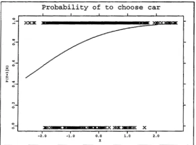
Probability of to choose car

-2.0 -1.0 0.0 1.0 2.0

Figure 1.1: Logit fit of the probability of individual choice of car for travel to work as function of transit fare minus automobile cost.

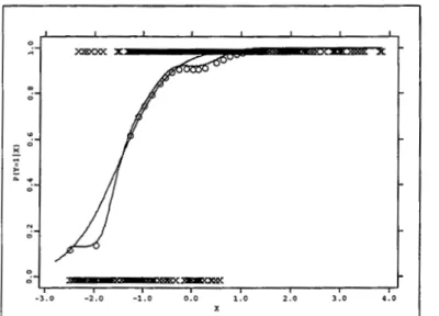
Fahrmeir and Thtz (1994) introduce an example of credit-scoring. The aim is to estimate the probability of an individual that has borrowed a credit amount is to be considered a potential risk by not paying back the debt as agreed upon by contract. As before the probability is a function of a set of covariates which influence the credit-ability of the individual here considered as risk factors. These covariates include, among others, the following: running account with categories no, medium, and good; duration of credit in months; amount of credit; payment of previous credits with categories good and bad; intended use, with categories private and professional.

Figure 1.2 shows a fit of the mentioned probability as function of the amount of credit borrowed for the data in Fahrmeir and Thtz (1994). The fit was obtained by logistic regression. The probability of a client constitute a potential risk increases with the amount of credit borrowed and is always below 0.8.

Later on, within the chapter, the assumptions underneath the models just presented will be discussed, alternative models combining the effect of sev-eral covariates will be examined as well. The economic motivation and in-terpretation of the binary model are discussed together with the alternative

''

., 0

..

- 0 ~ " _" 1::

..

~ 0 "' 0 -1.0

Probability of risky client

0.0 1.0 2.0 3.0 4.0 X

X

s.o

Figure 1.2: Logit fit of the probability of a client to be a potential risk as function of the amount of credit borrowed.

strictly econometric formulation. Parametric models like the probit, random-coefficients probit, logit and complementary log-log are analyzed.

The particular decision or attribute of the individual can be expressed by a random variable (the dependent variable) assuming only the values 0 or 1. When the individual has to choose in a set of more than two mutually exclusive alternatives or may verify one among more than two attributes the response is no longer binary. Models for categorical responses other than binary are much more complex. While this thesis concentrates on binary response models this chapter gives also a general overview of other categorical response models.

At the end of the chapter four different simulated data sets are introduced. They will be used during the work to illustrate the applicability of the methods in study.

1.2 The Utility Function Approach

The binary choice model can be derived from utility theory. This approach is very popular among econometricians due to its clear economic insight and can be found for instances in Amemiya (1981, 1983), Hausman and Wise (1978),

10 CHAPTER 1. PARAMETRIC BINARY MODEL

Judge, Griffiths, Hill, Liitkepohl and Lee (1985), and Train (1986).

In this approach the binary choice model is derived based on certain as-sumptions that define the behavior of the individual decision makers. Suppose that an individual decision maker is confronted with the choice between two different (and mutually exclusive) alternatives or attributes. For sake of clear-ness lets identify one alternative by I and the other by II. Economic examples are, among others, the choice of an individual to travel to work by automobile (alternative I) or by transit (alternative II), the choice of an individual to buy a certain product (alternative I) or not (alternative II), the choice of an individual to participate in the labor market (alternative I) or not (alternative

II), the choice of an enterprise to invest (alternative I) or not (alternative II).

The individual choice is represented by a random variable, Y,:, that assumes the value y;

=

1 if one alternative is chosen, say alternative I, or Yi

=

0 if the other is chosen, say alternative II.

Each individual has an indirect utility associated to each alternative rep-resented by an utility function. The utilities depend on the particular char-acteristics of the individual decision maker and the specific attributes of the alternative. Relatively to the example introduced about the probability of mode choice to travel to work one may assume that each individual has an utility associated with travelling by automobile and another utility associated with travelling by transit. Both utility functions depend on exogenous variables characterizing the individual like the number of cars owned by the household and the respective mode of travel like the time and fare of automobile for the first and the time and fare of transit for the second.

To simplify the specification of the individual utilities a common procedure used in economics and econometrics is based on the "representative individual" approach. This approach postulates the existence of a "representative" or "average" individual who is supposed to have tastes equal to the average over all individual decision makers. Let us assume that the indirect utilities of the "representative" individual associated to alternative I, say V1 , and associated

to alternative II, say Vo, depend on a set of exogenous variables z, representing the individual characteristics, and Wj with j

=

0, 1 corresponding to the specific

attributes of each alternative as faced by the individual according to

vl

=

V(z, WI, 'Y)

Vo = V(z, wo, 'Y) (1.1) where V( •) is a function known up to a vector of parameters 'Y with finite dimension. Usually one assumes that V( •) is a linear function.

It is further assumed that all individuals have a common structure in their

utilities which is the "representative" individual utility structure, that is the function V( • ). Moreover, the variation of the individual tastes from the "av-erage" is captured in the utility function only by a random component not observable.

Define the indirect utility of the ith individual associated to alternative

I for which Yi

=

1 as U1i and the indirect utility associated to alternative

II corresponding to Yi

=

0 as Uoi· The utilities of a given individual of the

population, say individual i, have two components. One, depends only on factors observable by the econometrician and has a common structure for all individuals equal to the utility of the "representative" individual. This part is referred to as the representative utility and expresses the average behavior of the population. The other, contains all influences that are unknown and gives the deviation of the individual tastes from the average behavior. This part is non-observable and random. Therefore, individual utilities are stochastic.

According to the above reasoning the utilities of individual i can be ex-pressed as

uli

=

V(zi,Wli,l)+fli

Uoi

=

V(zi, Woi, 1) + foi (1.2)

where V(•) are the representative utilities and fji, j

=

1,0, are random

vari-ables representing the stochastic part of the utilities which reflect the random tastes of the individual.

The aim is to fit the probability that the ith individual chooses alternative I, that is P(Yi = 1). The individual i will choose alternative I if the indirect

utility associated to it is greater than the indirect utility associated to the other alternative. The aimed probability becomes _P(U1i

>

Uoi) or according to (1.2) P{e-li-foi

>

V(zi, Woi, 1)-V(zi, wli, 1)} (1.3)

This probability depends on the distribution of the individual utilities, more precisely, on the distribution assumed for the deviation of the random tastes,

fli - foi. Then

(1.4) with G( •) the distribution function of fli - foi. To conclude, the specification

of the binary choice model depends on the particular function assumed for the representative utilities, V( • ), and the particular distribution assumed for the random utilities or more precisely the distribution G( •).

12 CHAPTER 1. PARAMETRIC BINARY MODEL

1.3 The Latent Variable Model

The binary choice model can be formulated by a latent variable model as in Maddala (1983). Suppose that underlying the choice variable

Yi

which assumes the values 1 or 0 there is a real-valued random variable Y;* known as the latent variable, such that

Yi 1 if Yi

>

0

Yi

=

0 otherwise (1.5) The usual approach assumes that the latent variable has a linear behavior defined by the relationship

where Xi is a vector of observable exogenous random variables taking values in

JRk which express the individual and the alternative characteristics, and Ui is a real-valued non-observable random variable whose stochastic structure will be examined later. From now on we will assume that

Yi*

has the linear behavior given in last equation.

The probability that individual i chooses alternative I given the values observed for the exogenous variables is,

P(Yi = 1IXi =xi)= P(Y;*

>

OIXi =xi)= P(ui

>

-xff3) (1.6)

In practice the latent variable Y;* is non-observable. Furthermore, to esti-mate the probability model (1.6) is not necessary to know the particular value assumed by the latent variable. In the following it will be shown how the latent variable is related to the individual utilities which are very difficult to observe in real situations.

The latent variable model and the formulation based on the utility theory are closely related. Assuming that the representative utility in (1.2) is linear then the deviation in the representative utilities of individual i becomes

where /O are the elements of 1 that are coefficients of the variables in Zi in

utility Uoi, 11 are the elements of 1 that are coefficients of the variables in Zi

in utility U1i and

t

are the remainder elements of 1 which are the coefficients

of variables in Wji, j

=

0, 1. Consider that 11 -'Yo and

t

constitute the vector

of parameters (3, that the vector of exogenous Xi is formed by variables Zi

"'

--~---~---(like the number of cars owned by the household in the running example) and

( Wli - wo;) (like transit travel time minus automobile travel time and transit

travel fare minus automobile travel fare in the mentioned example) and finally put f l i - <o;

=

u;,

with

x;, u;

and

/3

as in model (1.6). With this change of variables the deviation of representative utilities presented above becomes just

xf

{3 and consequently the probability that Uli

>

U0; in equation (1.3) reduces

to P( Ui

>

-xT

{3) which is also the probability P(Y/

>

OIX; = x;) in equation

(1.6). Therefore the distribution G( •) of f l i -<o; conditional on X; = x; is the distribution function of u; conditional on the same variable. From now on each time the distribution of u; or f l i -<o; is referred to the distribution conditional on X;

=

x; of those random variables is meant.

Note that the linear function

xf

{3 can be generalized in order to include some interaction terms or known transformations of explanatory variables. These interactions and transformed variables are treated merely as new exoge-nous variables enlarging the vector of explanatories x;. Also, except if stated otherwise, it is assumed that x; has as first element 1 in order to include an intercept term.

Very often the probability of choosing alternative I (1.4) is defined with respect to the distribution function of <oi - £1i or equivalently to the distribution of -u; normalized by a certain "convenient" variance resulting in the function

F(•).

Considering a sample of n individuals and assuming that their random utilities are all identically distributed the binary choice model is defined by

P(Yi =!IX;= x;)

=

F (

x~/3)

i

=

1, · · ·,n

with o-2 _{the variance of}

u; weighted by the particular variance that scales F( • ). In practice we are not able to identify o-2 _{which is absorbed by the coefficient}

values for the explanatories. Consequently, from now on, to ease the notation in the homoscedastic case where utilities are identically distributed, the coef-ficients

f3

are supposed to be normalized by o-. This amounts to consider that the probability of choice is given simply by the equation

P(Yi

=

!IX;= x;)

=

F(xf !3) i = 1, · · ·, n (1. 7)

The analysis of equation (I. 7) suggests some comments. First, the rela-tion with equarela-tion (1.4) reveals that the probability of choice of an alternative depends only on the difference in the individual utilities associated to each alternative and not on their absolute value. Consequently the choice of ex-planatory variables is restricted to the choice of variables that describe the

20 CHAPTER 1. PARAMETRIC BINARY MODEL

ordered or sequential. Because the focus of this thesis is on binary response models the survey in this section has not the aim to provide a deep and detailed study but to give a general overview on models for multinomial responses.

As before, the individual will choose the alternative that maximizes his utility and utilities have a deterministic part giving the representative utility or the average behavior and a unobserved and random part which is the deviation in individual tastes from the average behavior.

Suppose that the individual i faces m different and mutually exclusive al-ternatives. Let Pji

=

P(Yi

=

jjX;

=

x;), j

=

1, · · ·, m, be the probability that individual i chooses alternative j and assume that this probability is a function of linear indexes according to Pji

=

Fj(xfd3, · · ·, x'f'n;/3), with Xji, j

=

1, · · ·, m, a vector with explanatory variables with the same dimension as {3. One can as-sume that the observations for the responses, Yi, are arising from a multinomial distribution defined on m different categories where category j has probability Pji for individual i.

Parametric models assume a known form for Fj ( •) and the estimation of the probabilities of interest is reduced to the estimation of the parameters {3 by the maximum likelihood method. To obtain the maximum likelihood estimator it is useful to define the following set of dummy variables

Yii 1 if Yi = j

Yji 0 otherwise j = 1, · · ·, m i = 1, · · ·, n

Then the log likelihood function may be written as

n m

l

=

L LYii log Pji (1.17)

i=l j=l

Maximization of the log likelihood (1.17) is much more complicate than the maximization of the log likelihood of the binary model. The complexity de-pends also on the particular parametric model considered for Fj(•) and on the structure of the alternatives or attributes (whether they are unordered, ordered or sequential). Details can be found for example in Amemyia (1983).

1.6.1 Unordered Multinomial Models

An example of unordered alternatives can be found in Hausman and Wise (1978). The problem they study is the individual choice of mode to travel to work. Individuals face three alternatives: driving the own car, sharing rides, and riding a bus. There is no order relation between these alternatives.

The most common model in this problem is known as the multinomiallogit model. The multinomiallogit is often used in practice because the calculations necessary to obtain the maximum likelihood estimates are simpler than in other common parametric models like the multinomial probit. The model verifies,

exp(x'[iP) j=1,···,m-1 m-1 1

+

2:

exp( x'[iP) i=1 1 (1.18) m-1 1

+

2:

exp(x]iP) i=1

Amemyia (1983) shows how the multinomiallogit can be derived from utility maximization.

The multinomiallogit assumes that random utilities related to each alterna-tive are independent. This assumption implies that alternaalterna-tives are dissimilar. Suppose that an individual in choosing the transportation mode to work is faced with the alternatives own car, bus, and train. The probability of driving the car is P1

=

P(U1

>

U2, U1

>

U3) with U1, U2, U3 the utilities associated to driving the own car, riding by bus and riding by train. The multinomiallogit assumes that the events (U1

>

U2) and (U1

>

U3) are independent meaning that riding by bus has no common characteristic for the individual with riding by train. However those alternatives are not completely dissimilar given that both represent public transportation. Consequently, the multinomial logit is underestimating P1 because it ignores that if the individual prefers the car to the bus and u1

>

u2 makes u1

>

u3 more likely.

McFadden has called this characteristic of the multinomiallogit the "inde-pendence from irrelevant alternatives" (IIA) (McFadden, 1981). When some alternatives are similar a model should be used that to some extent does not verify this property. This is the case for the generalized extreme-value (GEV) model and the conditional probit (already referred to for the binary problem). The first model is derived assuming that random utilities have a GEV dis-tribution and has as particular formulations the nested logit model and the higher-level nested logit model described in Amemyia (1983). The second as-sumes that random utilities have a join normal distribution with a certain covariance matrix allowing for correlation among different alternatives and is described in Hausman and Wise (1978).

24 CHAPTER 1. PARAMETRIC BINARY MODEL

coefficients st. errors

Intercept -1.2216 0.3022

Number of cars 2.3081 0.2243 Out-of-vehicle travel time 0.0622 0.0173 In-vehicle travel time 0.0092 0.0095

Travel cost 0.0169 0.0021

Table 1.1: Results of the logit fit on the problem of mode choice for travel.

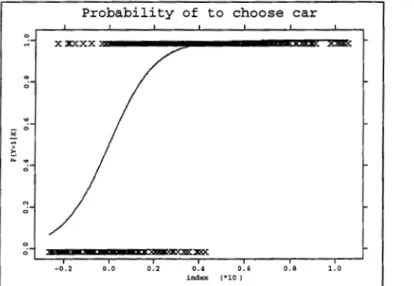
by the household, transit travel time relatively to automobile and transit fare relatively to automobile costs although in-vehicle travel time may not be sta-tistically significant to explain the probability of choice. Figure 1.4 shows the logit fit for this example. Now the probability curve is plotted against the fitted index. m 0 N 0 -0.2

Probability of to choose car

0.0 0.2 0.4 0. 6 0.8 1.0

index {*10 )

Figure 1.4: Logit fit of the probability of individual choice of car for travel to work.

Table 1.2 shows the estimates obtained for the logit fit of the credit-scoring data while the fit is plotted in Figure 1.5. The probability of a client to be considered a potential risk is a function of the duration of credit in months, payment of previous credits with values 0 for good and 1 for bad, amount of

coefficients st. errors

Intercept -1.6232 0.3428

Duration of credit 0.0253 0.0078 Payment of previous credits 1.2900 0.2359 Amount of credit 0.0001 0.0000 Monthly payment 0.2080 0.0734

Age -0.0215 0.0069

Table 1.2: Results of the logit fit on the problem of credit-scoring.

credit, percentage of monthly payment in the individual income and age of the client. The probability of a client to be a potential risk grows with the duration of credit, a bad payment of previous credits, the amount borrowed and the weight of the monthly payment on individual income. On the other side the probability decreases with the age of the client.

.,

0

N

0

0

Probability of risky client

Xli!::ZWi!iC! _ _ _ _ _ _ _ _ _ CEl!ll!t =xx

o XXX»•

-2.0 -1.0 o.o 1.0

index

26 CHAPTER 1. PARAMETRIC BINARY MODEL

1.8

An Example

This section introduces four simulated data sets which differ in the link function considered. These data sets will be used in the remainder of this thesis to illustrate the reasoning of the methods to be presented. They are described in the following.

Four parametric models were considered for the conditional probability of choice of alternative I, F(xf (3) according to,

F(xf (3) F(x[ (3) F(x[ (3) F(xf (3) s(x[ (3) {1+exp(-x[(3)}-1 (1.21) 1- exp{-exp(x[ (3)} (1.22) { 1 + exp -xi ( Tf3)}-l +

"""1.5

-xr

f3

x

T.5

1.25 x <p (xf

T.5 ,

{3) ( )

1.23 [ 1 + exp {

s(:J :) }

rl

(1.24) (1

+

lx[

(31)112

with <p( •) the standard normal density.

Models (1.21) and (1.22) are classic parametric models, the logit and the CLL. Model (1.23) is a logit model perturbed by a bump with height given by 1.25 and width equal to 1.5. The value 1.25 was chosen such that the conditional expectation of

Yi

will never decrease when

xf

(3 increases. Finally, model (1.24) is a logit model with heteroscedasticity where the heteroscedasticity is given by the function s(

xr

(3).

These models were chosen because they may be considered typical to char-acterize some frequent situations that may arrive in problems with binary re-sponses.

The logit model is the most used for problems with no presence of hetero-geneity in data which are well depicted by a symmetric link while the CLL is a popular alternative model when a non-symmetric link is required.

The logit with bump link in (1.23) is a deviation from the logit link which make the conditional probability function to be flatter on a neighborhood of the index function centered at zero as can be seen in the lower left plot of Figure 1.6. In that region the link has an increasing rate almost equal to zero. Mind that the index function translates the difference in the utility associated to each alternative. In general it may be interpreted as the difference in the score assigned by the individual to each alternative. Consequently, when the index is around zero it means that the score allocated by the individual to each

alternative is very similar. It is natural to think that individuals have some difficulties to decide which alternative to choose in those cases. This behavior can be translated by a weak increase of the cumulated conditional probability of choice, or by the flatness of the link function, in the region where the index assumes values around zero and can be represented by the logit with a bump link in (1.23). On the other side, this model can be viewed as giving merely an alternative behavior of individuals relatively to the logit where individuals prefer more strongly alternative one under an unfavourable score (when the index assumes negative values) and prefer it less under a favourable score of this alternative relatively to the other (when the index assumes positive values) than those individuals behaving according to the logit model.

The logit with heteroscedasticity represents a deviation from the logit model that incorporates heterogeneity among individuals by considering an heteroscedas-tic latent variable or heteroscedasheteroscedas-tic stochasheteroscedas-tic utilities. The presence of het-erogeneity among individuals may be relevant in practical situations. See as example the application on mode-choice of travelling in the way to work of Horowitz (1993).

For all experiments the index function was assumed to be 1 - xil

+

2xi2 and the number of observations was set to 500. The regressors were generated independently from a standard normal. For sake of comparison the same data set for the regressors was used in all experiments to generate the response from a Bernoulli distribution with probability of success given respectively by mod-els (1.21) to (1.24). Thus, individual i has explanatory variables with the same magnitude in all data sets, with i

=

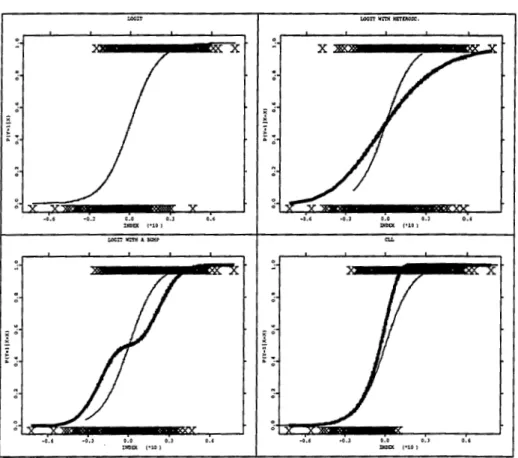
1, · · ·, 500. On the othr hand, the endoge-nous variable was generated using the same random seed in all experiments.

Figure 1.6 shows the four models introduced. The logit with a bump (lower left), the logit with heteroscedasticity (upper right) and CLL (lower right) are plotted together with the logit model.

In practice the true link function is unknown and a common behavior is to assume that data come from a logit specification. Assuming a logit link results in a misspecification when estimating data sets generated by models (1.22), (1.23), and (1.24).

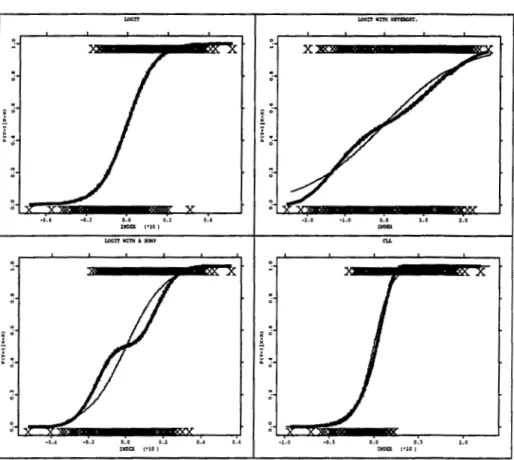
Figure 1. 7 shows the shapes of the introduced models with the parametric logit fit obtained in each data set respectively. The logit fit was plotted against the estimated index,

xT

p,

while the true models were plotted against the true index

xT

f3

(which is the same in all experiments according to what was said before). The upper left shows data generated from the logit estimated assuming a logit. The fit and the true model are coincident. All the other plots in the

28

CHAPTER 1. PARAMETRIC BINARY MODEL

~o., 0.0 O.l -0.6 •O,l o.o o.J

...

IHD~ 1'10) OOEX 1•10)

tDCIT WITH A lUMP ttJ. KOD£1.

'·'

Figure 1. 6: Upper left- the logit model, lower left- the logit with a bump (thick line) and the logit, upper right- the logit with heteroscedasticity {thick line} and the logit, lower right - the complementary log-log and the logit. The values for the response generated by the model in the plot are identified by crosses.

figure show misspecified fits.

A feature to remark in Figure 1. 7 is that the length of the fitted index for the misspecified models in the upper right and lower left, identified in the figure by the range of the support of the logit fit, shows a tendency to underestimate the range of the true index. This happens because in fact the variance of the latent is different in all models given that f3 is the same for all but each link is defined for a different scale. When estimating the data with a logit link the estimates of the standard deviation of the latent will automatically scale the estimates of f3

(weighted by the the standard deviation of the logistic distribution). Therefore, the scale of the estimates for f3 or equivalently the scale of the fitted index, has

''

''

1.8. AN EXAMPLE 29 X o.o o.J INDCt 1•101 -0.6 -0.3 0.0 O.J '·' INDEX !"10 l

Figure 1. 7: Upper left- the logit model, and logit fit, lower left- the logit with a bump (thick line) and parametric logit fit, upper right- the logit with heteroscedasticity {thick line) and parametric logit fit, lower right- the complementary log-log and parametric logit fit. The values for the respective response in each plot are identified by crosses.

to be different in each specification.

Plots in Figure 1.7 may lead to an erroneous judgment of the kind of the deviation the logit fit has from the true model. To compare this deviation one has to normalize the fitted index or alternatively the true index in order that j3 and

/3

are in the same scale by making the necessary adjustments with the standard deviations of the true and the logit links. Figure 1.8 shows the plots with the true index normalized by dividing by the standard deviation of the respective true link and multiplying by the standard deviation of the logit link. The CLL was also adjusted in location.

30 CHAPTER 1. PARAMETRIC BINARY MODEL

"""' LOOlT WITH KITDOtC,

-0.6 o,o O,J '·' o,o

,,,

"' "'"" ('10) 11/DIX l.OCIT MlTH A BUMP "" '·' -1.0 o.o 0,5 1.0 INDEX (0_{10 1} INDEX !'10)

Figure 1. 8: Upper left - the logit model, and logit fit, lower left - the logit with a bump {thick line) and parametric logit fit, upper right- the logit with heteroscedasticity {thick line} and parametric logit fit, lower right- the complementary log-log and parametric logit fit. The values for the respective response in each plot are identified by crosses. Index normalized.

link is not captured by the ill-specified parametric fit. The upper right shows the logit with heteroscedasticity. Note that plotting the probabilities against the index divided by the heteroscedastic variance function modifies the shape of the curve. Now the curve shows a bump which is not captured by the logit fit. However the deviation is not so great as in the case before. In the lower right the CLL model with misspecified logit fit is given. Here, the misspecification of the fit is not explicit given that the true CLL model is very close to the logit fit.

The plot in the lower right shows that the location of the CLL is very well

1

\ ', 1 'I

:J

,I

I t J

'I

II

'j

!1

1

!J

'

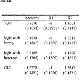
intercept X1 X2 logit 0.7870 -1 1.4601 (0.1093) (0.12235) (0.1413) logit with 0.4933 -1 1.3317 bump (0.1557) (0.1669) (0.1733) logit with 0.5162 -1 1.1725 heterosc. (0.1704) (0.1809) (0.1821) CLL 1.2772 -1 1.5647 (0.1321) (0.1220) (0.1571)

Table 1.3: Results of the logit fit on the simulated data. Standard errors inside brackets.

estimated by the logit fit. Mind that the location is absorbed into the estimate of the constant term. The logit with a bump and logit with heteroscedasticity links are referred to the same location as the logit. Thus, is natural that the logit fit of data from those models has no location inaccuracy as the figure shows.

All the plots show that the spread of the fitted index is very close to the spread of the normalized true index which induces that the misspecified logit fit is able to assess correctly the variance of the latent variable (though it is not identifiable in practice). Mind that in the plots in the lower left the true index was normalized by multiplying f3 by a constant while in the lower right it was normalized by adding a constant and multiplying by another. Therefore one can conclude that in those examples the slope coefficients in f3 are well ap-proximated up to a proportional constant by the respective elements of

/3.

This subject will be examined later on in the next chapter. For the heteroscedastic-ity case in the upper right the same conclusion holds if one considers that the heteroscedasticity is reflected in the distortion of the logit link as is shown in the plot. More precisely, the function s( •) is absorbed into the link which then is not anymore a logit as in the right upper plot of Figure 1.6.

Table 1.3 shows the logit estimates for the coefficients f3 in the four data sets introduced. The estimates are normalized from being divided by the absolute value of the coefficient estimate of the first regressor in order to be on the same

32 CHAPTER 1. PARAMETRIC BINARY MODEL

scale for the different data sets. The logit fit was implemented in XploRe 3 using the GLM module. The estimates are not much different except the estimate of the intercept of the CLL model which is clear larger than the others.

However, even if the misspecified logit fit gives accurate estimates of the slope coefficients in

f3

up to a constant the true probability curves are deviat-ing from the logit fit because of not takdeviat-ing into account the existence of bumps in the link for the logit with a bump and logit with heteroscedasticity mod-els. When data are generated by the CLL model it is hard to distinguish the difference between the true link and the misspecified parametric estimate by a merely inspection of their plot. However, that distance may be assessed using another tool like a test statistic.

This work aims to study and to improve tools that allow to detect mis-specification on the link function of a binary choice model by evaluating if the deviation between a parametric estimate of the link and the true function is statistically significant in the sense that is not due only to sample randomness.

.,

'i

~I

,.,

The Semiparametric Binary

Choice Model

2.1

Introduction

In chapter 1 some parametric binary choice models were introduced. First, models that do not allow for the existence of heterogeneity on tastes of the individuals were focused. These are the logit, probit, and CLL. While results are almost the same whether probit or logit are used this is not the case with the CLL. Second, heterogeneity among individuals was introduced with the RCP model. Here heterogeneity appears as heteroscedasticity verifying a very particular parametric form namely the variances of the latent variables Y;* are given by xTI:.xi with I:. a k X k positive definite matrix.

All the parametric models are derived based on distributional assumptions of the latent variable Y;* (or equivalently of the random utilities). These as-sumptions are somehow restrictive since they imply certain behavior of the individuals and may induce misspecification of the parametric model. In this case, maximum likelihood estimates may be inconsistent or inefficient engen-dering predictions about the individual choice that can be entirely wrong.

To be robust to the kind of misspecification mentioned above one can define a model where no assumptions (or very few) are made about the distribution of the latent variable. In this chapter a model will be presented that fulfills this aim. It widens the parametric assumptions about the individuals behavior in order to be more general and more flexible than the parametric models

34 CHAPTER 2. SEMIPARAMETRIC BINARY MODEL

presented within a semiparametric approach. It also includes the parametric models as particular cases. This model is recognized in the literature as single index model (SIM) and can be applied to a wide class of problems from which binary responses are just a particular case.

The specification of the semiparametric model and its estimation will be addressed within the chapter. The estimation methods that are yn-consistent are privileged for reasons that will become more clear in the subsequent chap-ters. The construction of confidence bands based on the semiparametric fit will be also discussed and introduced as a first tool to compare a parametric model with the semiparametric rival.

2.2

The model

The semiparametric model can be viewed as a generalization of the paramet-ric model. The purpose of the semiparametparamet-ric approach is to widen the as-sumptions regarding the link function F( •) while avoiding the curse of dimen-sionality that is hampering fully nonparametric techniques when applied to high-dimensional data. The semiparametric model overcomes the curse of di-mensionality by aggregating the multidimensional variable Xi into the single

(parametric) index

xr

/3,

while maintaining the nonparametric assumption that the specification of the link in equation (1.9) is unknown. A SIM formulation of the binary choice model can be seen for example in Stoker (1992).

The single index model for binary responses takes on the following form

E(Yi\Xi =xi)= P(Yi

=

1\Xi =Xi)= F(x[

/3)

i

=

1, · · ·, n (2.1) with F(•) an unknown ("smooth") function with range contained m [0, 1] which, as in (1.9), is not necessarily a distribution function.

The SIM may incorporate heterogeneity in tastes across individuals if it is manifested as heteroscedasticity. The heteroscedasticity is of unknown form and has to depend on the index function. To make more clear note that model (2.1) can be written

i

=

1, · · ·,n

with g(•) assuming values on [0, 1], u(•) always positive, and both unknown functions. Here, if u( •) is not equal to a constant it can be seen as the variance function of a heteroscedastic latent variable. In practice the function u( •) is not identifiable and it is absorbed into the unknown link resulting in F( • ). The

·''

.

' I ~I

.

' .,

'i

I ':

2.3. SEMIPARAMETRIC ESTIMATION OF THE SIM 35

main restriction of the SIM model (2.1) is the linearity of the utility functions or the linearity of the latent variable Y;*.

In the SIM the intercept is not identifiable and it is subsumed in the link function. Note that the mean of the random part of the latent variable, more precisely the mean of the variable -u; with u; as in (1.5), is unknown. When the link F( •) is parametric it has a known fixed location which may not be the true mean of -Ui. The difference between the fixed location in F( •) and the

true mean of -u; is given by the intercept of the model. Thus, in parametric models the intercept is normalized not only by the scale imposed to the link but also by its fixed location. For example, probit and logit models have fixed location equal to zero therefore the intercept gives the mean of -u; for a given scale. Because in the SIM F( •) is free there is not an automatically fixed location allowing to identify the intercept which is instead absorbed in F( • ). The same will happen to the scale. That is, because F( •) is unknown it can not impose a natural scale and location for the index like in parametric models. To conclude, for parametric models the link F( •) is defined for a given location and scale which fixes a natural normalization for the coefficients

/3,

that is the scale and the intercept value. In the SIM the procedure is inverse. Because the link is unknown it is necessary to define a convenient normalization for

f3

exogenously which fixes naturally the scale and location of the link F( •). This means that scale and location will be absorbed into the link.

One strategy to normalize the vector

f3

consists on fixing the intercept equal to zero and one of the other component coefficients equal to 1. This will be

the nor~alization used in this work. Therefore, the vector of coefficients

f3

(without intercept) is uniquely identified up to a multiplicative constant. From now on it will be considered that the vector of coefficients

f3

in the SIM has no intercept.

2.3

Semiparametric estimation of the SIM

Estimation of the semiparametric model (2.1) proceeds in two steps. First, the coefficient vector

/3

has to be estimated. Let us call this estimate

/3

and

xf

j3

the estimated index. The second step estimates the link function by smoothing the data Yi on the projected index

x[

/3.

The smoother used in this work is the

38

N

0

-1.0

CHAPTER 2. SEMIPARAMETRIC BINARY MODEL

Probability of risky client

o.o 1.0 2.0 X

3. 0 4. 0 s.o

Figure 2.2: Probability curve of a client being a non potential risk as function of the amount of credit borrowed: logit fit and kernel regression.

2.3.1 WADE Estimator

This method is a modification of average derivative estimation (ADE) (Hardie and Stoker, 1989). ADE is motivated by the following property of single index models of the form (2.1)

E{\7 F(x;)} = E (

d~;f3)

(3 =

1f3

where the expectation is taken with respect to the distribution of X; and

\7 F(x;) =oF/ax;.

Assuming that F( •) is a.e. first differentiable in X;, (3 can be estimated up

to a constant by estimating the mean of the gradient vector \7 F(x;). On the other hand, if \7 F(x;) is proportional to

f3

then any weighted average of the derivatives \7 F(x;) will also be proportional to (3. Let w(x;) be a weighting function. Then

This equation motivates the WADE procedure. The aim is to choose a con-venient weight function in order to make the estimation of the mean of the

'

weighted gradient vector easier than the estimation of the mean of its

un-weighted counterpart. Powell et al. (1989) show that this is accomplished if

the weight function is the density function of X;.

Suppose that X; is continuously distributed with density p(x;) which is also differentiable. Put w(x;) = p(x;). Under some suitable regularity conditions (see Powell et al., 1989) integration by parts allows to write

E{p(xi)'v F(x;)}

=

-2E{Yi'Vp(x;)}. (2.5)

with 'Vp(x;) the gradient vector of p(x;). Therefore, estimating

f3

up to a constant amounts to estimate the derivative of the density of X;.

Given a sample of n individuals the WADE estimator (with weight p(x;)) for a constant times (3 is given by

A 2~

-d = -L... Yi 'Vp(x;).

n i=l

(2.6)

The estimate of the gradient of the density of X; is obtained by kernel smoothing. For theoretical reasons the estimate at point x; omits the ith observation in the smoothing process according to

vP(

X;)

=

n

~

1

t. (

~)

k+l f{' (Xi

~

X j )

Jr•

where k is the number of explanatory variables in X;.

Powell et al. (1989) show that dis asymptotically normal distributed with asymptotic covariance matrix consistently estimated by

where A 4~ T " T I:d = - LJ r(xi)r(x;) - 4dd n .

•

n ( ) k+l ( ) A 1 1 ,, Xi- Xj

r(xi)

=

n _ ₁

~

h

A h (y;-Yj)

Jr•

(2.7)

Note that WADE can be applied only to "continuous" explanatory variables. That means, categorical regressors or dummy variables cannot be included in the model. For some problems this can be an undesirable restriction.

2.3.2 Maximum Quasi-Likelihood Estimator

Klein and Spady (1993) propose as estimate of

f3

the value that maximizes the log likelihood of the binary choice model (1.14) when F(x[ (3) is substituted

40

CHAPTER 2. SEMIPARAMETRIC BINARY MODEL

by

Fhi(xT

/3) a nonparametric kernel regression with bandwidth h, calculated excluding observation i and usually known as leave-one-out (100) kernel re-gression. The 100 estimator is defined by,

n

2::

I< { (

v - xJ

/3) /

h}

Yi ~ 'f:.' Fhi( v)

=

3'-'-:~:--- (2.8)

L

I<

{(v- xJ/3)/h}

#i

where all the variables have the same meaning as before.

The introduction of the above estimate in the likelihood function results in a so-called quasi-likelihood. For theoretical purposes the authors introduce a trimming in the quasi-likelihood to eliminate observations with imprecise estimators of F( •). In practice the trimming has revealed to be not important and can be omitted.

The maximization of the quasi-likelihood is performed iteratively in the same way as any nonlinear function. Bonneu, Delecroix and Malin (1993) advise to consider for the bandwidth h in each iteration the value

s(xT

iJ)n-1₁5

where

s(xr

i3)

is the sample standard deviation of the index

xr

i3

i

=

1, ... , n with

i3

the actual estimate of

f3

in that iteration.

Klein and Spady (1993) prove the asymptotic normality of the quasi-likelihood estimator

/3.

They show that

vn(/3-

/3) ..!:..., N(O, ~) with

{( oF) (oF)T

1

}-1

~

=

E

o/3

o/3

F(1 - F) (2.9)

To estimate the covariance matrix ~ it suffices to plug-in in (2.9) the stan-dard estimates of the unknowns, respectively

f3

and F and take the sample mean. Because the information equality between the negative of the Hessian matrix and the expected outer product gradient still holds in this problem the covariance above can be also estimated with White's (1982) estimator. Note that for inference purposes the quasi-likelihood may be treated like an usual likelihood function. Therefore, the estimates for the variance of the coefficients returned by a conventional likelihood routine are still valid. On the other side the classic likelihood ratio tests can be performed in the same manner with the quasi-likelihood as with a likelihood function.

Klein and Spady (1993) show that the maximum quasi-likelihood estimator is asymptotically efficient under the assumption of independence of the random component of the latent variable, Ui, and the regressors.