A Work Project, presented as part of the requirements for the Award of a Masters Degree in Finance from the NOVA – School of Business and Economics.
MODELING AND FORECASTING VALUE-AT-RISK FOR THE PORTUGUESE STOCK MARKET
ANDREIA SOFIA DA SILVA RODRIGUES, 679
A Project carried out on the Finance course, under the supervision of: Iliyan Georgiev
MODELING AND FORECASTING VALUE-AT-RISK FOR THE PORTUGUESE STOCK MARKET
ABSTRACT
The aim of this work project is to find a model that is able to accurately forecast the daily Value-at-Risk for PSI-20 Index, independently of the market conditions, in order to expand empirical literature for the Portuguese stock market. Hence, two subsamples, representing more and less volatile periods, were modeled through unconditional and conditional volatility models (because it is what drives returns). All models were evaluated through Kupiec’s and Christoffersen’s tests, by comparing forecasts with actual results. Using an out-of-sample of 204 observations, it was found that a GARCH(1,1) is an accurate model for our purposes.
1
1. INTRODUCTION
“Nothing ventured, nothing gained” is what leads investors to take risks, as higher potential return requires taking higher risk. However, sometimes the probability of losses is higher than, or just as high as, gains. Therefore, risk – “volatility of unexpected outcomes” (Jorion, 2007:3) - must be managed and measured carefully. One of the most popular methods is designated as Value-at-Risk (VaR): a risk management tool that puts a monetary (or percentage) value in the potential maximum loss one can incur in, when holding an asset, for a predefined time horizon, at a given confidence level.
Companies, financial institutions or individual investors are exposed to several types of risk, but this work project will focus on market risk, which refers to the potential losses that come from variations on securities, such as stocks’ market prices. According to Jorion (2007), the market risk of holding portfolios with various stocks (each one with different sources of risk) must be evaluated, and the best way to do it is using VAR. Note that, in the context of this work project, it will be set as a percentage value, instead of monetary, which is well approximated by a stock continuously compounded return1.
Nowadays, there are several approaches one can follow to estimate VaR, which have been improving over time, in order to provide both simple implementation and precise estimations (usually there is a trade-off). In the present thesis, two perspectives will be evaluated: unconditional (simple) and conditional volatility models (sophisticated econometrics ones) of returns2. Hence, one of the hypotheses tested in this thesis is:
The use of sophisticated econometric models provides advantages in VaR predictions over simpler ad-hoc methods.
1 Returns represent the economic gain (positive return) or loss (negative return) of an investiment/portfolio,
being a good approximation for percentage VaR.
2
2
Although evolving, one of main challenges regarding forecasting in finance continues to be whether the models applied are able or not to anticipate changes in the market volatility, as in the recent financial crisis in 2008 that certainly led to changes in the stock market conditions all over the world. This issue is also tested in this work project:
( ) There is one model approach which provides good one-day VaR forecasts, independently of the actual market conditions.
As one of this work project intents is to expand empirical research for the Portuguese stock market, which has little or no space into the literature so far, to test those hypotheses, a sample from PSI-20 Index daily returns will be collected and afterwards divided into (i) before and after 2008 crisis subsamples and an (ii) out-of-sample evaluation period, which corresponds to the present year of 2014 (until October 17th). In the end, one expects that some of the findings of this thesis can be useful for the Portuguese risk managers to improve the way they forecast risk and better protect the Portuguese institutions against any unexpected negative event.
Finally, in order to validate these models, the actual losses/gains of PSI-20 Index in 2014 will be compared to the ones predicted by each model (technique designated as
backtesting), where the likelihood ratios of unconditional (or Kupiec) and conditional (or
Christoffersen) coverage tests are the methods applied for this end.
Note that, one of the thesis limitations is the lack of comparison data and the assumption that the modeling and analysis of PSI-20 Index returns are good enough to provide empirical findings that can be applied in any type of assets in Portugal.
2. LITERATURE REVIEW
Value-at-Risk (VaR) is a statistical tool that summarizes a portfolio’s “worst loss over a target horizon such that there is a low, prespecified probability that the actual loss will
3
be larger” (Jorion, 2007:106). By convention, VaR is set as a positive number – percentage, in this case – hence:
(1)
where is the actual daily PSI-20 Index return and α is the “prespecified probability” which we call significance level. Recall that VaR, in this work project context, is being established as a percentage. Therefore, according to the standard time-series modeling of daily returns:
(2) where is the mean for returns, is the squared-root of - the volatility for returns - and is a series of independent and identically distributed (i.i.d.) random variables with mean 0 and variance 1 (Tsay, 2002). However, daily changes in prices are not systematically positive or negative, which means that daily returns are usually not significantly different from zero. This is why, in the literature, daily VaR is stated as:
(3) To better understand VaR definition, consider the following illustration: if, for a 95% confidence level, daily VaR is €100.000,00 one interprets it as having 5% probability (or being 95% certain) that tomorrow’s loss will (not) be higher than €100.000,00.
One of the most widely used VaR estimation approaches is the Historical Simulation (HS). Under HS assumptions, past distribution of returns is a good proxy for its future distribution, which is not true if market conditions change. This was one of the findings of a study carry out by Beder (1995). He analyzed two samples of the U.S. Treasury Strips returns – with the previous 100 and 250 days – and found that the HS method predicted an appreciation of the Treasury strips, when it should not, since the selected
4
estimation windows corresponded to “a period of rising interest rates” (Beder, 1995:15) i.e., the U.S. market conditions were changing, which HS did not captured.
As it does not rely on any parameter estimation, HS is also denominated as a
non-parametric technique. In 1996, Hendricks compared one-day VaR predictions provided
by HS and two parametric approaches - equally and exponentially weighted moving averages -, considering four data set periods with 125, 250, 500 and 1250 days of several currencies’ exchange rate against the dollar. His study’s results showed that “the best performer is the 1,250-day HS approach (…) while the worst performer is the 125-day HS approach” (Henndricks, 1996:50), meaning that HS for “longer horizons provide better estimates of the tail of the distribution” (Hendricks, 1996:47). However, for HS to be an accurate model, it may require too aged data, which may be irrelevant to explain the current market behavior of the period under analysis, as showed by Beder (1995).
To overcome this HS drawback, research over parametric models, which do not require such long periods of historical data, increased. Here, a theoretical distribution of returns, given their past behavior, is assumed known. According to Brooks, “financial assets returns tend to exhibit leptokurtic distributions” (2008:380), which predicts more extreme returns (fatter tails) that the Normal distribution. Xiong and Idzore went even further by finding that “extreme events seem to occur 10 times more often than the normal distribution predicts” (2011:23). Given that, and because Student’s t distribution has fatter tails than the normal, the parametric Student’s t is also a common technique adopted for forecasting VaR purposes. In order to assess the advantages of this technique, Huisman at al. (1998) compare the results between parametric-normal and parametric Student’s t VaR approaches. Their study was composed by bi-weekly data of S&P 500 Composite Returns Index and US 10-Year Government Bond Returns Index. According
5
to Huisman at al. results, not only Student’s t characteristics fit better the distribution of returns, but it is also true for more than one asset’s type, since “for both US stocks and bonds, the VaR-x3 estimates reflect the true downside risk apparent in financial returns much better than those from the standard4 VaR estimators” (1998:59).
In the end, all of those were reasons for parametric Student’s VaR model to emerge in the literature as preferred instead of the normal. Nevertheless, note that both HS and parametric Student’s t VaR assume that returns have constant volatility – the so-called unconditional volatility models. However, as stated by Brooks (2001:380), financial data has a stylized characteristic of volatility clustering i.e., returns have time-varying volatility. To overcome that, Bollerslev (1986) suggested a generalized autoregressive heteroscedastic (GARCH) process that, not only is able to capture the leptokurtosis, but also the volatility clustering of the returns distribution. Nevertheless, according to GARCH models, positive price shocks have the same impact in the volatility of returns as negative ones. However, there is empirical evidence for shocks to have asymmetric effects over prices: negative shocks have greater impact than positive ones (Brooks, 2008:380). Therefore, to capture such asymmetry effects, two extensions of GARCH widely used in the literature - exponential GARCH and GJR-GARCH -, were suggested by Nelson (1991) and Glosten at al. (1993), respectively.
Regarding the performance of these three models, past studies are not unanimous: Ramasamy and Munisamy concluded that, when forecasting exchange rates’ volatility, “the leverage effect brought in GJR and EGARCH models do not improve the results of GARCH much” (2012:98). In the other side, for Tel-Aviv stock market, according to
3 VaR-x is their notion for parametric Student’s t VaR. 4
6
Alberg et al., “the asymmetric GARCH model with fat-tailed densities improves overall estimation for measuring conditional variance” (2008:201). In fact, as different types of assets have different statistical characteristics, it seems difficult to find a model that suits and captures all of those properties accordingly. Thus, it will be interesting to find which conclusion, of the two (if any), one is able to reach in this thesis.
3. METHODOLOGY 3.1.Data: PSI-20 Index
As the aim of this work project is to find a method of VaR calculation that works effectively in the Portuguese stock market, regardless of the financial market conditions, PSI-20 Index was the proxy chosen as the most relevant for the purposed analysis since it already corresponds to a well-diversified portfolio with stocks of the major 20 Portuguese companies. Furthermore, financial assets must be evaluated at their market value, and because the stocks composing PSI-20 Index are traded on a daily basis, the information about its current market price is publically available. Given that, the day-to-day returns (net of dividends) from January 2nd, 2002 to October 17th, 2014 were collected from Bloomberg, where the period from (i) 2nd January 2002 to 31st December of 2007 is the Before Crisis period subsample; (ii) 2nd January 2008 to 31st December of 2013 is the After Crisis period subsample and (iii) 2nd January to 17th October of 2014 is the out-of-sample forecasting period.
As seen before, there are 3 factors one has to establish in order to calculate VaR: i. Time horizon: The one-day VaR implies the use of daily returns for the models to be coherent. For management purposes, the access to prompt information is crucial, which means that, if one only updates prices’ information weekly or monthly, it might miss some trends in the data that could have been important to anticipate an event and
7
protect against it. Nevertheless, one of the inconveniences daily data is the fact of requiring a lot of historical data, which loses relevance the older it is, because market conditions are constantly. According to Zangari and Bayraktar (2005/2006), the drawbacks of analyzing daily returns do not overcome the benefit of precision it offers, being the reason why daily returns were preferred.
ii. Probability Distribution Function: According to Xiong and Idzore, “extreme events seem to occur 10 times more often than the normal distribution predicts” (2011:23). For that reason, it is not accurate, just for simplicity, to assume that PSI-20 Index returns follow a normal distribution. Firstly, although almost symmetric, returns’ empirical probability distribution function is skewed (asymmetric do the left – negative skewness - or to the right – positive skewness) and leptokurtic (has fatter tails, which means that more extreme returns are likely when compared to the normal distribution5). Since Student’s t distribution, although symmetric, has fatter tails than the Normal, it will be the conditional distribution of returns, given their past, assumed. However, note that their unconditional distribution can exhibit asymmetry and even heavier tails than a Student’s t because it is given by (equation (3)). Therefore, even though are Student’s t distributed, they are being multiplied by (which is a random variable in the estimation models), so the distribution of their product will no longer be Student’s t. iii. Confidence Level: As it is a more subjective parameter, it will be defined as both
Basel Committee on Banking Supervision – according to Basel III (Latham&Watkins, 2011:53) – and RiskMetrics (JP Morgan and Reuters, 1996:37) consider it. Hence, the 99th and 95th one-day VaR percentiles will be set in order to also compare, respectively, a more conservative approach towards risk with one less risk averse.
5
8
3.2.Unconditional VaR Models
These models postulate that returns are stationary, which implies that the unconditional moments of the series are constant or non-varying over time. In practice, it means that in equation (3), where is the daily standard deviation of the returns’ sample. Under these restrictions, a non-parametric (Historical Simulation) and a parametric unconditional VaR models will be presented. These will be the ‘simpler ad-hoc methods’ category, as they are the easiest to implement.
3.2.1. Historical Simulation
A classic approach to compute VaR is the Historical Simulation (HS). HS is a non-parametric approach, in the sense that it does not require the use of statistical methods to estimate any parameter since it uses the empirical distribution of returns. As it assumes that historical returns are a good proxy for future returns forecasts, HS implicitly assumes that returns are strictly stationary6. It is a strong assumption once market conditions are constantly changing and, consequently, the distribution of PSI-20 Index returns today will most likely not be the same as before the 2008 financial crisis.
According to this method, VaR is calculated as:
(4) where is the -quantile of the returns’ empirical distribution (the lowest return of all observations, where is the number of observations) and is the expected value of returns, estimated by their sample average.
3.2.2. Unconditional Parametric Student’s t VaR Model
Recall Equation (3). For now, and, in practice, is assumed to follow a determined probability distribution function. As explained in the previous section, it is
6
9
not expected returns to follow a normal distribution, so that Student’s t is being assumed, which expresses returns as:
(5)
where is the threshold value of the cumulative Student’s t distribution with α
probability mass to the left and ν degrees of freedom. The model is denominated as
parametric because, although assumed known, the (Student’s t) distribution of still
depends on the degrees of freedom parameter, which needs to be estimated.
Besides the fact of seeing both mean and standard deviation of returns as constant over time, the fact of assuming one probability distribution function of returns that may be wrong is another drawback of this forecasting method, since it leads to higher forecasting errors by undervaluing or overvaluing the predicted VaR.
3.3. Conditional VaR Models
Stationarity restricts the unconditional moments of the returns time series (section 3.2.); however it allows for the conditional moments to vary in time. Moreover, empirical evidence supports that it is not accurate to assume constant volatility, as summarized in the following “stylized facts” (Brooks, 2008:380):
i. Clustering: there is empirical evidence that days with high (low) volatility are followed by days with high (low) volatility, so there is positive autocorrelation between the conditional variance of returns in a given day and its lags.
ii. Serial dependence (or persistence): empirically, volatility appears to have long memory, i.e., returns from a long period ago seem to have some explanatory power over the current variance forecast (specially for daily returns);
iii. Leverage effects: in the stock market (and in general), negative shocks (‘bad news’) have a greater impact on volatility than positive shocks (‘good news’) do.
10
Thus, conditional volatility means that the volatility forecasts at time – the values plugged in in equation (3) – are conditional on the information (Ω) that is available at time , i.e. (6) In order to be able to model volatility, one needs more advanced econometric models as GARCH, EGARCH and GJR that are able to capture the aforementioned dynamics. Moreover, the coefficients of these models will be estimated through an advanced software package – EViews –, as well as the tests to verify their accuracy.
3.3.1. Generalized Autoregressive Conditional Heteroscedastic Models
Bollerslev (1986) expressed the conditional variance as a function of past shocks and its own lags. In this work project, only one-day lag of each is being modeled, being designated as GARCH(1,1):
(7) where to ensure non-negative variance (note that, for we are before an ARCH(1) type model). Although this model is able to account for volatility clustering by including variance lags, GARCH(1,1) has some limitations. Firstly, the non-negativity restrictions can be violated. Furthermore, it does not capture the asymmetry effects explained previously since all the shocks, according to (7), have the same absolute impact on volatility (shocks are squared).
3.3.2. Glosten, Ravijagannathan and Runkle (GJR) Models
Consider the following extension of equation (7) to express the conditional variance, denominated as GJR-GARCH(1,1) or GJR(1,1), suggested by Glosten at al. (1993):
(8) Here, is a dummy variable equal to 1 if and to 0 otherwise. Moreover, and ensure a non-negative variance, which allows to be
11
negative but not higher than . However, it usually is positive to account for asymmetry, because when a positive shock happens, the term including the dummy vanishes and we stick to a simple GARCH(1,1) model; but if it is negative, the dummy variable is “activated” increasing the forecasted conditional variance and the expected VaR.
Although the asymmetry dynamics are captured by GJR, the non-negativity constraints can still be violated, which is why exponential GARCH is introduced.
3.3.3. Exponential Generalized Autoregressive Heteroscedastic Models
The EGARCH(1,1) expression for the conditional variance, suggested by Nelson (in 1991) has the following form:
(9)
The model has two main advantages over GARCH(1,1): first, ensures the non-negativity constraint for the variance, thus no restrictions on the parameters are necessary. Secondly, leverage (or asymmetry) effects are taken into account through γ. To account for leverage effects, γ must be negative: when there are ‘bad news’ (negative shocks), it augments volatility, and the expected loss will be higher; and when there are ‘good news’, the volatility decreases and so does the expected VaR.
Note that the coefficients of GARCH(1,1), and its extensions, are estimated through maximum likelihood estimation, by maximizing the log-likelihood function . Here, the assumption for the returns conditional distribution becomes crucial, since depends on its density function. Thus, for the Student’s t distribution: (10) where is the gamma function.
12
In these cases, because all models are highly non-linear, no expressions for the coefficients can be derived from first order conditions, therefore numerical optimization has to be the method adopted instead.
3.4. Backtesting
In this section, the accuracy of all methods applied to forecast VaR is tested through the unconditional and conditional coverage tests, where the predicted VaR is compared to the actual loss. For both tests, we have: VaR model is adequate.
3.4.2. Unconditional Coverage Test (Kupiec’s Test)
Recall Equation (1): VaR is being estimated assuming α% probability of being exceeded, which means that the expected exception rate is α%, being the total number of exceptions. An exception, can be interpreted as a dummy variable where is equal to 1 when and to 0 otherwise, thus (11) where the number of observations in the out-of-sample forecasting period.
Consider the following example: for a 95% confidence level, the expected is 5%. If one considers a sample of 1000 days , then should be days.
The unconditional coverage test, developed by Kupiec (1995), tests whether the number of VaR exceedances is statistically equal to the expected one where the following likelihood ratio is the test statistic:
(12)
Under the null hypothesis, follows a Chi-Squared distribution with 1 degree of freedom ( , so if is higher than critical values, the model is not accurate.
13
3.4.3. Conditional Coverage Test (Christoffersen’s Test)
One of the previous test limitations is the fact of not taking into account whether the exceptions are concentrated or dispersed over time. Firstly, one expects an exception to happen once in a while (to be dispersed), otherwise if exceptions do occur 2 or more days in a row, it would mean that VaR forecasting model applied is not able to capture some market risk changes. Secondly, it is also expected that an exception today does not depend on whether an exception happened in the previous day or not, i.e. it is expected exceptions to be independent and spaced over time. Hence, to overcome this Kupiec’s test flaw, Christoffersen (1998) implemented the temporal independence test, which test-statistic is a likelihood ratio:
(13)
where is the number of times (recall that 1 corresponds to the exception) on day was followed by on day . Moreover, is the exception
rate, is the exception rate conditional on no exception in the previous day and is the exception rate conditional on exception in the previous day.
Given that, the overall likelihood ratio of the conditional coverage
test not only verifies if the exception rate is equal to the expected one, but also if it is independent on whether an exception happened yesterday or not . Its test statistic is:
(14) Under the null hypothesis, follows a Chi-Squared distribution with 2 degrees of freedom ( , so if is higher than critical values, the model is not accurate.
14
4. EMPIRICAL RESULTS
Intuitively, it seems relevant to subdivide the overall sample into two periods: one pre crisis (2002-2007) and one post crisis (2008-2013), as the stock market behavior was different between the two. However, is it statistically relevant to analyze two different subsamples to estimate the daily VaR for PSI-20 Index?
Consider the following equation, which is an extended version of (8):
, (15)
where is a dummy variable equal to 0 if January 2nd, 2002 December 31st
, 2007 and equal to 1 if January 2nd, 2008 December 31st, 2013. According to Table 1, none of the parameters individually (except for 5% significance level) are statistically significant. However, one must perform a joint significance test, with the following hypotheses: and .
Table 1: Joint Significance of Equation (14) Dummy Variables
According to maximum likelihood, the test statistic for a joint significance test is the following likelihood ratio:
(16)
which, under the null hypothesis, follows a Chi-Squared distribution with 3 degrees of freedom .
According to Table 1, there is no statistical evidence, for 5% and 1% significance levels, to reject the null hypothesis since is higher than the respective critical values of . Thus, it is appropriate to distinguish two subsamples.
Coefficient -0.021 (0.0397) -0.052 (0.022) -0.0063 (0.004) p-value 0.59 0.02 0.078 Log-Likelihood Null Hypothesis: Log-Likelihood
Notes: The critical values of are, respectively for 1%
and 5% significance levels, 11.34 and 7.82. The standard errors are in parentheses.
15
4.1. Descriptive Statistics
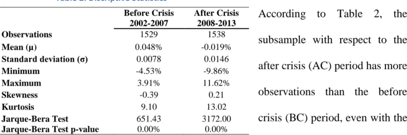
Table 2: Discriptive Statistics
According to Table 2, the subsample with respect to the after crisis (AC) period has more observations than the before crisis (BC) period, even with the same length in years. The main reasons for that are: (i) some holidays that coincided with weekends in BC period, may have not in AC period and (ii) in 2013, some holidays were suspended, so there were more business days in Portugal, in the AC period.
As expected, the average of daily returns and the daily standard deviation are different as the samples describe different market characteristics: BC period has a higher average of daily returns ( of 0.048% which contrasts with of -0.019%), while the AC
period, where the markets were very unstable, is a much more volatile one ( of 0.0146
against of 0.00778).
Regarding the normality of the returns distribution, and in agreement with the stylized facts of returns, one can conclude that, in both cases, it is not normal. First, although almost symmetric, both subsamples are slightly skewed: while the BC period is negatively skewed (-0.39), the AC one is asymmetric to the right (positive skewness of 0.209). In other words, most of the probability is around the mean of returns, meaning that the difference between the samples’ distributions is in the tails: BC has less probability mass spread to negative returns (left to the mean) while the AC period has less mass probability of positive gains (right to the mean). Secondly, both subsamples are also leptokurtic ( of 13.02 and of 9.10). This result is also not
surprising since, the AC period being a more volatile one, has more extreme results
Before Crisis 2002-2007 After Crisis 2008-2013 Observations 1529 1538 Mean (µ) 0.048% -0.019% Standard deviation (σ) 0.0078 0.0146 Minimum -4.53% -9.86% Maximum 3.91% 11.62% Skewness -0.39 0.21 Kurtosis 9.10 13.02 Jarque-Bera Test 651.43 3172.00
16
(range between -9.86% and 11.62% against the BC period range between -4.53% and 3.91%) and, as we stated in the previous section, the more extreme returns results, higher the probability mass left to the tails, thus more leptokurtic. The ultimate confirmation for the non-normality of the series’ distribution is the performance of the Jarque-Bera test. According to Table 2, in both subsamples, the test’s p-value is 0.00%, which means that we strongly reject, for both significance levels, the hypothesis of PSI 20 Index returns being normally distributed.
4.2. Models Estimation
Table 3: Unconditional VaR Models Forecasts
According to Table 3, the parametric (refer to Appendiz 1 for more details concerning the estimation of the degrees of freedom, ) Student’s t predicted VaRs, for both significance levels in both subsamples, are higher than HS ones. As the main limitation of assuming a theoretical distribution of returns is the possibility of being the wrong one, it seems that the t-student distribution is a conservative approach regarding PSI-20 VaR predictions, since it overvalues it when compared to HS.
Regarding the conditional volatility VaR models, one must assure that the order chosen (or the fitted model) is adequate for our purposes. According to Tsay, it “can be checked by using the standardized residuals” (2001:95). The standardized residuals are i.d.d. random variables assumed to follow a standardized Student’s t distribution – recall equation (3) –, therefore one can examine the series (Tsay, 2001:89) which must have no evidence of serial dependence nor ARCH effects.
Before Crisis After Crisis
5% 1% 5% 1%
α-Percentile -1.23% -2.34% -2.35% -4.09%
Historical Simulation (HS) VaR 1.28% 2.39% 2.33% 4.07%
3.6 3.6 4 4
2.35 3.75 2.13 3.75
17
Table 4: Ljung-Box Test (30th Lag) for Autocorrelation in Squared Standardized Residuals
Before Crisis After Crisis
GARCH(1,1) 28.01 0.57 32.42 0.35
EGARCH(1,1) 30.16 0.46 33.24 0.31
GJR(1,1) 28.2 0.56 28.82 0.53
Primarily, to test for serial dependence, the Ljung-Box Q-Stat Test was applied over the standardized squared residuals where the null hypothesis is no serial dependence (or ). Given that, until 30 lags of squared residuals’ autocorrelations were jointly tested and, according to Table 4, since the p-value of the test is highly above 1% and 5% significance levels, we do not reject the null, in any model. So, there is no evidence of serial dependence in the series.
For models to be true, they must also be able to capture all volatility dynamics present in the data, which means that standardized residuals should have constant volatility (no ARCH effects). Therefore, an ARCH-Heteroscedasticity test was also performed. Here, under the null hypothesis ( No ARCH Effects), the test statistic – Langragian Multiplier – follows a Chi-Squared distribution with 1 degree of freedom . If is not significant (p-value higher than the significance levels) or smaller than the critical values of , we do not reject the null hypothesis.
Table 5: Test for ARCH Effects in Standardized Residuals
Before Crisis After Crisis
GARCH(1,1) 0.47 0.49 0.029 0.87
EGARCH(1,1) 0.76 0.38 0.007 0.93
GJR(1,1) 0.74 0.39 0.49 0.48
Notes: For 1% significance level, the critical values of and are, respectively,
6.64 and 9.21. For 5% significance level, they are 3.84 and 5.99, respectively.
According to Table 5, there is no statistical evidence to reject the null, in any model, since the test statistic has p-values highly above 1% and 5% significance levels, which means that is no ARCH effects – standardized residuals have constant volatility.
18
As there is no evidence of serial dependence nor extra ARCH effects in series, the order (1,1) for GARCH, and its extensions, is well defined and their coefficients estimates should be consistent, efficient and accurate for forecasting purposes.
Table 6: Estimated Coefficients for Conditional Volatility Models
GARCH (1,1) GJR(1,1) EGARCH (1,1)
Coefficient p-value Coefficient p-value Coefficient p-value
B ef o re C ris is 5,3E-07 (2,5E-07) 0,019 1,04E-06 (3,41E-07) 0,0023 -0,419 (0,094) 0,00 0,063 (0,013) 0,00 0,041 (0,014) 0,0033 0,181 (0,03) 0,00 (0,014) 0,929 0,00 0,912 (0,022) 0,0021 0,97 (0,008) 0,00 - - 0.069 (0.069) 0,00 -0,06 (0,018) 0,001 6 (0.86) 0,00 6 (0.893) 0,00 6 (0.898) 0,00 Af ter C ris is 9.1E-06 (2.7E06) 0.001 0.00001 (2.4E-06) 0,00 -0.54 (0.102) 0,00 0.131 (0.023) 0.00 0.029 (0.021) 0.1662 0.18 (0.033) 0,00 0.823 (0.029) 0,00 0.83 (0.028) 0,00 0.95 (0.0103) 0,00 - - 0.18 (0.034) 0,00 -0.12 (0.018) 0,00 (2.197) 10 0,00 13 (3.83) 0.0009 14 (4.29) 0.002
Notes:The standard error are presented in parentheses
According to Table 6 – where the numbers in the brackets are the standard errors –, all coefficients are strongly significant, as their p-values are below 1%, excepting at 1% significance level, estimated via GARCH(1,1) using the BC subsample GARCH and , for both significance levels, estimated VIA GJR(1,1) using the AC subsample. This implies that, it makes sense to set up such expressions to model conditional volatility, since one-day lag for both residuals (recall: except GJR) and conditional variance are significant to describe the behavior of the current conditional variance.
What is more, GARCH effects, , measure the persistence of shocks. Overall, volatility shocks for all models have long memory, i.e. they will have an impact on the future conditional variance forecasts, since varies around 0.82-0.97 (the closer to 1, the higher the degree of persistence). Among the models, volatility is, by far, more
19
persistence when estimated via EGARCH(1,1), for both subsamples ( of 0.95 of
0.97), while estimated through GARCH(1,1) and GJR(1,1) varies around 0.82-0.93. Secondly, being significant in all the scenarios leads us to conclude that returns react differently towards positive and negative PSI-20 volatility shocks. Consequently, and because it does not capture asymmetry effects in the PSI-20 Index returns’ series, GARCH(1,1) model is not suitable to fit its theoretical distribution. Moreover, recall sections 3.3.2. and 3.3.3., for EGARCH(1,1) model, is negative in both sub-samples ( of -0.0596 and of -0.116) while for GJR(1,1) it is positive ( of 0.069 and of 0.177), reinforcing the existence of leverage effects throughout the series.
4.1. Models Diagnoses
Some important conclusions were taken from the previous sub-section, however one still have to test whether the models are accurate or not for the aim of this project.
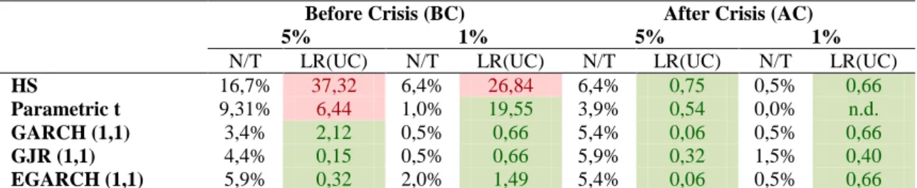
Table 7: Unconditional Coverage (Kupiec's) Test
Table 8: Conditional Coverage (Christoffersen's) Test
For better interpretation of results, Table 7 and Table 8 are divided into red, for rejected models, and green, for the models found to be accurate for VaR predictions.
Before Crisis (BC) After Crisis (AC)
5% 1% 5% 1%
N/T LR(UC) N/T LR(UC) N/T LR(UC) N/T LR(UC)
HS 16,7% 37,32 6,4% 26,84 6,4% 0,75 0,5% 0,66
Parametric t 9,31% 6,44 1,0% 19,55 3,9% 0,54 0,0% n.d.
GARCH (1,1) 3,4% 2,12 0,5% 0,66 5,4% 0,06 0,5% 0,66
GJR (1,1) 4,4% 0,15 0,5% 0,66 5,9% 0,32 1,5% 0,40
EGARCH (1,1) 5,9% 0,32 2,0% 1,49 5,4% 0,06 0,5% 0,66
Notes: For 1% significance level, the critical values of and are, respectively, 6.64 and 9.21. For 5%
significance level, they are 3.84 and 5.99. The test was based on a forecasting sample size of 204 observations.
Before Crisis After Crisis
5% 1% 5% 1%
LR(Ind) LR(CC) LR(Ind) LR(CC) LR(Ind) LR(CC) LR(Ind) LR(CC)
HS 6,27 43,59 9,49 36,33 8,13 8,87 n.d. n.d.
Parametric t 17,08 23,53 n.d. n.d. 1,07 1,61 n.d. n.d.
GARCH (1,1) n.d. n.d. n.d. n.d. 2,46 2,52 n.d. n.d.
GJR (1,1) 0,73 0,88 n.d. n.d. 5,12 5,44 n.d. n.d.
EGARCH (1,1) 5,12 5,44 n.d. n.d. 0,26 0,33 n.d. n.d.
Notes: For 1% significance level, the critical values of and are, respectively, 6.64 and 9.21. For 5%
20
Note also that, for 1% significance levels, the independence test shows not defined (n.d) results and there are two main reasons for that: first, the sample size is too short to find two exceptions in a row. Secondly, 1% significance level is too conservative, allowing for scarce exceptions and making it difficult to find two exceptions in a row.
Table 9: Fisher’s Exact Independence Test (p-values)
To solve this limitation, Fisher’s Exact
Test is an alternative independence test one
can resort to. It is mostly employed in small samples and provides the exact p-value from a hypergeometric distribution (contrarily to the p-value based on the Chi-Squared distribution which is only an approximation). According to Table 10, we strongly do not reject the null hypothesis of independence, as p-values are all close (or even equal) to 1. Due to the complexity of this test, refer Appendix 8 for more detailed information about the method it follows.
Given that, a straightforward conclusion can be taken: as the unconditional VaR models are more often rejected than the conditional volatility ones, the assumption of volatility being constant, as expected, is rejected. Moreover, it seems that the estimated coefficients from the AC subsample provide better forecasts of VaR in 2014 than the ones estimated from the BC subsample. Here, we have two perspectives: primarily, the observations of the AC subsample are more recent whereas the BC subsample includes observations from 12 years ago. Given that, as the stock market conditions have changed in the last 7 years – especially for Portugal that also faced a huge crisis in investors’ expectations since International Monetary Fund intervention – such old data may have little or no power to explain how it behaves today. In the other hand, one can also interpret these results as evidence that Portugal is still living the repercussions of the mentioned drawbacks, not having recovered yet from them.
Before Crisis After Crisis
5% 1% 5% 1% HS - - - 0.999 Parametric t - - 0.999 1.000 GARCH(1,1) 1.000 0.999 - 0.999 GJR(1,1) - 0.999 - 1.000 EGARCH(1,1) - 0.999 - 1.000
21
According to Kupiec’s test (Table 7), both parametric Student’s t – excepting at 1% significance level – and HS models, for the BC period, underestimate VaRs for 2014, since they present exception rates above 12% (when it should have been 5%) and 5% (when it should have been 1%). When a financial crisis happens, the markets become much more volatile given the uncertainty a new situation implements. Being more volatile means higher probability of losses, hence if both unconditional models set up a VaR that is too low, it means they are unable to anticipate probable higher losses. In the other hand, for the AC period, both models seem to be accurate for VaR predictions, for both significance levels. Regarding the conditional volatility models, all models seem to produce accurate VaR forecasts, as their exception rates are aligned with the expected ones, using the coefficients estimated from both BC and AC subsamples.
Regarding Christoffersen’s test (Table 8), BC parametric Student’s t, at 5% significance level, and HS (except, at 1% significance level) unconditional models, failed the independence test. As their VaR predictions led to too many exceptions, the probability of them being in a row increases, mainly when the out-of-sample size is small. At the end of the day, and although they are not a good fit for the PSI-20 Index returns’ theoretical distribution, both parametric Student’s t VaR (except for the BC subsample, at 5% significance level) and HS, via AC subsample, at 1% significance level, models turned out to be accurate to forecast VaR,. When it comes to the conditional volatility VaR models, all of them passed the conditional coverage test. However, VaR predictions given by EGARCH(1,1) using the coefficients estimated from the BC subsample and by GJR using the ones estimated from the AC subsample, did not passed the independence test, at a 5% significance level. Note that, the aim of this work project is to forecast VaR, instead of returns. Thus, characteristics as time-varying
22
volatility or asymmetry effects, that are relevant when testing how well the models fit the returns theoretical distribution, may not be significant to improve forecasts of VaR, as suggested by both coverage tests’ results. This is why HS, parametric Student’s t and GARCH(1,1) models are still able to provide good VaR forecasts, even though they do not capture all the dynamics present in the series.
Moreover, recall that one of this work projects’ aims is also to find a model able to generate good VaR predictions using the estimated coefficients of both subsamples ( ). According to Kupiec and Christoffersen, all models - excepting HS -, at 1% significance level – and GARCH(1,1) also at 5% – are able to do so. Note that, these tests are not structured to make comparisons between the models, just to evaluate the accuracy of each one. So, for comparison purposes, Jose A. Lopez suggested a backtesting procedure not based “on a hypothesis-testing framework” method (1999:7), contrarily to the previous two, designated as Loss Function . A particular form of this method is:
(17) which not only addresses if the actual loss, at time exceeded the predicted VaR (which, recall, would be scored as 1), but also the exceedance’s magnitude, by adding the 2 term. As generates individual scores for each daily VaR forecasts, the average loss for the forecasting sample is given by: (18)
Table 10: Average Loss for the Forecasting Sample
Because the closer the prediction is to its true value, the smaller the exceedance’s magnitude, the model providing the lowest is preferred. Hence, according to Table 10, VaR estimates generated by GARCH(1,1),
Before Crisis After Crisis
5% 1% 5% 1% HS 0.51 0.5 0.52 0.5 Parametric t 0.5 0.5 0.5 0.5 GARCH(1,1) 0.034 0.05 0.004935 0.004931 GJR 0.044 0.004934 0.059 0.015 EGARCH(1,1) 0.059 0.02 0.054 0.004933
23
EGARCH(1,1) –using the coefficients estimated from the AC subsample – and by GJR(1,1) – using the coefficients estimated from BC subsample –, produce the lowest average losses (the estimated VaR exceeds, on average, its true value by 0.00049). These results also lead to the conclusion that, for the Portuguese stock market, asymmetry effects do not offer improvements in VaR estimates, being irrelevant for that aim. Given that, GARCH(1,1), especially at 1% significance level, is a sufficient model to forecast VaR for the PSI-20 Index because, although by an almost immaterial difference, has the lowest average loss of all.
In the other hand, the unconditional VaR models provide the highest average losses. Although, under certain assumptions, HS and parametric Student’s t are accurate models to predict VaR, the fact of not capturing the time-varying volatility seems to lead to a higher forecast error, so that modeling it may improve the results after all.
5. CONCLUSIONS
The aim of this work project was to find a useful model for the Portuguese risk managers more accurately predict one-day Value-at-Risk for 2014. For that purpose, two hypotheses were tested, and the conclusions are:
1. Hypothesis is rejected: One of the most interesting findings of this work project was, in fact, to conclude that misspecified models – which do not capture all the returns’ series dynamics – are able to produce acceptable VaR estimates. Recall that VaR is just the th
or 99th percentile of the returns’ distribution, so it is possible to correctly specify such quantile’s distribution but misspecify the whole one. Therefore, even though parametric Student’s t VaR does not account for time-varying volatility and GARCH(1,1) does not capture the asymmetry effects present in the data, both models provided good VaR estimates for PSI-20 Index.
24
2. Hypothesis is not rejected: According to the unconditional and conditional coverage tests, all the conditional volatility VaR models and parametric Student’s t , at 1% - and GARCH(1,1) also at 5% - significance level, are able to produce accurate VaR predictions using both before and after crisis subsamples’ estimated coefficients.
Moreover, according to Loss Function based backtest results, VaR estimates of GARCH(1,1) - at both significance levels - and EGARCH(1,1) at 1% significance level (using the coefficients estimated through the after crisis subsample) and GJR(1,1), at 1% significance level (using the coefficients of the before crisis subsample) generate, on average, practically the same deviation from the actual loss. Therefore, including asymmetry effects is not relevant for VaR forecasting purposes, in the Portuguese stock market, as modeling conditional volatility through EGARCH(1,1) or GJR(1,1) does not provide any advantages over GARCH(1,1). Besides, as conditional volatility models outperform the unconditional ones - because the exceptions generated by HS and parametric Student’s t VaRs are, on average, higher than the ones from the remaining models -, one can conclude that accounting for time-varying volatility is relevant for PSI-20 Index, as it improves its VaR estimates.
6. REFERENCES
Alberg, Dima, Haim Shalita, and Rami Yosef. 2008. “Estimating stock market volatility using asymmetric GARCH models.” Applied Financial Economics, 18(15): 1201-1208
Beder, Tanya S. 1995. “VAR: Seductive but Dangerous.” Financial Analysts Journal, 51(5): 12-24.
Bollerslev, Tim. 1986. “Generalized Autoregressive Conditional Heteroskedasticity”
25
Brooks, Chris. 2008. Introductory Econometrics for Finance. 2nded. New York: Cambridge University Press.
Christoffersen, Peter F. 1998. “Evaluating Interval Forecasts.” International Economic
Review, 39(4): 841-862.
Glosten, Lawrence R., Ravi Jagannathan and David E. Runkle. 1993. “On the Relation between the Expected Value and the Volatility of the Nominal Excess Return on Stocks.” Journal of Finance, 48(5): 1779-1801.
Hendrick, Darryll. 1996. “Evaluation of Value-at-Risk Models Using Historical Data.”
Federal Reserve Bank of New York Economic Policy Review, 39-70.
Huisman, Ronald, Kees G.Koedijk and Rachel A.J. Pownall. 1998. “VaR-x: Fat tails in financial risk management.” Journal of Risk, 1(1): 47-61.
Jorion, Philippe. 2007. Value at Risk: The New Benchmark for Managing Financial
Risk. 3rd ed. New York: The McGraw-Hill Companies.
Kupiec, Paul H. 1995. “Techniques for Verifying the Accuracy of Risk Management Models.” Journal of Derivatives, 3(2): 73-84.
Lopez, Jose A. 1999. “Methods for Evaluating Value-at-Risk Estimates.” Federal
Reserve Bank of San Francisco Economic Review, (2): 3-17.
Nelson, Daniel B. 1991. “Conditional Heteroskedasticity in Asset Returns: A New Approach.” Econometrica, 59(2): 347-370.
Ramansamy, Ravindran and Shanmugam Munisamy. 2012. “Predictive Accuracy of GARCH, GJR and EGARCH Models Select Exchange Rates Application.” Global
Journal of Management and Business Research, 12(15): 89-100.