Breeze effects at a large artificial lake: summer case study

https://doi.org/10.5194/hess-22-5191-2018 © Author(s) 2018. This work is distributed under the Creative Commons Attribution 4.0 License.

Breeze effects at a large artificial lake: summer case study

Department of Physics, ICT, Institute of Earth Sciences, University of Évora, 7000 Évora, Portugal Correspondence: Maksim Iakunin (miakunin@uevora.pt)

Received: 12 April 2018 – Discussion started: 18 April 2018

Revised: 14 August 2018 – Accepted: 6 September 2018 – Published: 5 October 2018

Abstract. Natural lakes and big artificial reservoirs can af-fect the weather regime of surrounding areas but, usually, consideration of all aspects of this impact and their quan-tification is a difficult task. The Alqueva reservoir, the largest artificial lake in western Europe, located on the south-east of Portugal, was filled in 2004. It is a large natural laboratory that allows the study of changes in surface and in landscape and how they affect the weather in the region. This paper is focused on a 3-day case study, 22–24 July 2014, during which an intensive observation campaign was carried out. In order to quantify the breeze effects induced by the Alqueva reservoir, two simulations with the mesoscale atmospheric model Meso-NH coupled to the FLake freshwater lake model has been performed. The difference between the two sim-ulations lies in the presence or absence of the reservoir on the model surface. Comparing the two simulation datasets, with and without the reservoir, net results of the lake im-pact were obtained. Magnitude of the imim-pact on air temper-ature, relative humidity, and other atmospheric variables are shown. The clear effect of a lake breeze (5–7 m s−1) can be observed during daytime on distances up to 6 km away from the shores and up to 300 m above the surface. The lake breeze system starts to form at 09:00 UTC and dissipates at 18:00– 19:00 UTC with the arrival of a larger-scale Atlantic breeze. The descending branch of the lake breeze circulation brings dry air from higher atmospheric layers (2–2.5 km) and redis-tributes it over the lake. It is also shown that despite its signif-icant intensity the effect is limited to a couple of kilometres away from the lake borders.

1 Introduction

Human activities, such as urbanization, deforestation, or wa-ter reservoir building, change the properties of the surface (vegetation cover, emissivity, albedo) that rule the surface energy fluxes (Cotton and Pielke, 2007). As a consequence, changes in surface energy fluxes affect local weather and cli-mate. Lakes and reservoirs contain about 0.35 % of global freshwater storage (Hartmann, 1994) and cover only 2 % of the continental surface area (Segal et al., 1997). Thermal cir-culations triggered by lake–land thermal contrast have an impact on dispersion of air pollution and lake catchment transport (Lee et al., 2014). Big lakes, being a significant source of atmospheric moisture, can intensify storm forma-tion (Samuelsson et al., 2006; Lin et al., 2012). Lakes and reservoirs, compared to land surfaces, have higher thermal inertia and heat capacity, and lower albedo and roughness length (Bonan, 1995). They can affect meteorological condi-tions and atmospheric processes at mesoscales and synoptic scales (Pielke, 1974; Bates et al., 1993; Pielke, 2013).

Normally, near-surface relative humidity is increased while daily air temperature is decreased above lake and shore areas. During the warm summer periods the relatively colder lake surface interacts with the atmosphere above, which leads to a reduction in clouds and precipitation. Formation of the local high-pressure areas over the lake surface in the summer season supports atmospheric circulation, which can be ob-served as a lake breeze (Bates et al., 1993). In autumn and winter it has the opposite effect: due to the fact that wa-ter is warmer than the air above, increases in evaporation and cloud formation can be observed (Ekhtiari et al., 2017). These regional lake effects have been seen in previous stud-ies, e.g. Elqui Valley reservoir in Chile (Bischoff-Gauß et al., 2006) and the great African lakes (Thiery et al., 2014).

The theoretical aspects of lake breeze formations are well known; however, this phenomenon remains unexplored. Dif-ficulties in studies of lake breeze are due to the diversity and complexity of lake shapes and surrounding landscapes, and the lack of observational data at sufficiently fine spatial reso-lution (Segal et al., 1997).

Lake breezes are mainly determined by the landscape and weather conditions. Formation and intensity of the breeze de-pend on the set of parameters such as large-scale winds, sen-sible heat flux, geometry of the lake, and terrain types of the surrounding area (Segal et al., 1997; Drobinski and Dubos, 2009; Crosman and Horel, 2012).

The focus of this work is on the study of the lake breeze at the Alqueva reservoir and its impact on atmospheric pa-rameters of the surrounding area. This large artificial reser-voir was filled in 2004, which makes it a big natural labora-tory for studying physical, chemical, and biological effects. Few studies about the influence of Alqueva on atmosphere and climate were published. The first report, in Portuguese, was published even before the construction of the dam by Miranda et al. (1995), as a part of the environmental im-pact study of the reservoir on the basis of numerical sim-ulations performed with the NH3D (non-hydrostatic three-dimensional) mesoscale model from Miranda and James (1992). It was concluded that the climate impact of the multi-purpose Alqueva project should be mainly due to the irriga-tion of surrounding area. The influence of the reservoir itself was unclear as at that time it was not possible to perform high-resolution simulations. The studies were continued and improved by Salgado (2006) who made the first attempt to quantify the direct effect of the reservoir on the local cli-mate, in particular on winter fog. Using the Meso-NH (non-hydrostatic mesoscale atmospheric model) model, the author concluded that the introduction of the reservoir should in-crease the winter fog slightly in the surrounding area, but de-crease it over the filled area. Later on, Policarpo et al. (2017) used observations from two periods of 10 years (before and after the Alqueva reservoir) combined with Meso-NH simu-lations and showed a slight increase in the average number of days with fog during the winter (about 4 days per winter after 2003 in a downwind site).

Mesoscale atmospheric models, such as Meso-NH, al-low obtainment of results with adequate horizontal reso-lution (250 m in present study) for studying the local ef-fects of air temperature changes and the generation of small-scale circulations under different large-small-scale atmospheric sit-uations. In this work simulations have been run for the Intensive Observation Period (IOP) of the ALEX project (ALqueva hydro-meteorological EXperiment, http://www. alex2014.cge.uevora.pt/, 28 September 2018). Data collected during this experiment were used to validate the numerical simulations.

The article outline is as follows. Section 2 provides a brief description of the Alqueva reservoir. Section 3 introduces information about the ALEX experiment and the

measure-ments used in this paper. Section 4 contains a brief descrip-tion of the numerical models used in this work: Meso-NH and FLake. Sections 5 and 6 are dedicated to the case study on 22–24 July 2014: validation of simulation results using in situ measurements and the studies of the lake effects re-spectively, with an illustration and discussion of the magni-tude of the impact and intensity of a lake breeze. Section 7 summarizes the results and conclusions.

2 Object of study

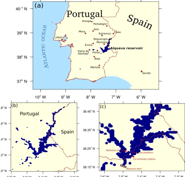
The Alqueva reservoir, established in 2002, is an artificial lake located in the south-east part of Portugal. It spreads along 83 km over the Guadiana river valley covering, when completely filled, an area of 250 km2 with a capacity of 4.15 km3, which makes it the largest artificial lake in western Europe (Fig. 1a). The maximum and average depths of the reservoir are 92 and 16.6 m respectively. The dam is located in the southern part of the reservoir (Fig. 1c).

The Alqueva reservoir is mainly used to provide water sup-ply, irrigation, and hydroelectric power. The region where it is located is known for the irregularity of its hydrological re-sources, with long periods of drought that could last for more than one consecutive year (Silva et al., 2014). The region has a Mediterranean climate with dry and hot summers (Csa ac-cording to the Köppen climate classification), with a small area within of the mid-latitude steppe (BSk) category. Dur-ing summer, the maximum air temperature ranges between 31 and 35◦C on average (July and August), often reaching values close to 40◦C, or even higher. The incident solar ra-diation at the surface is one of the highest in Europe, with mean daily values (integrated over 24 h) of about 300 W m−2 and the daily maximum in July often reaching 1000 W m−2. Rainfall periods are seasonal, normally from October to April. The annual average of accumulated precipitation in the climatological station of Beja, located 40 km away from the Alqueva reservoir, is 558 mm (1981–2010 normals from http://www.ipma.pt/pt/index.html, 28 September 2018).

Two major factors determine synoptic circulations over the region during the summer period: the shape and loca-tion of the Azores anticyclone, and the frequent establish-ment of a low-pressure system over the Iberian Peninsula, induced by the land–ocean thermal contrasts. The later phe-nomenon is known as the Iberian thermal low (Hoinka and Castro, 2003), which organizes the sea breezes generated at the Iberian coasts on a peninsular scale. At the west coast, the sea breeze controls the transport of the maritime air masses from the Atlantic to Iberian Peninsula, on distances more than 100 km reaching the Alqueva region in the late after-noon. This effect is observed in the local increase in wind intensity and in its rotation (Salgado et al., 2015).

Figure 1. Nested domains used in the simulations: (a) the “father” domain at 4 km horizontal resolution with 100 × 108 grid points, with location of the 12 IPMA synoptic stations used for validation; (b) intermediate 1 km horizontal resolution domain, 96 × 72 grid points; (c) finer 250 m resolution domain comprising 160 × 160 grid points, together with the location of the ALEX land stations, the Montante floating platform and the dam.

3 Measurement data

The measured data used in this work were obtained during the ALEX campaign – a multidisciplinary observational ex-periment at the Alqueva reservoir that lasted from June to October 2014. One of the aims of this project was to per-form a wide set of measurements of chemical, physical, and biological parameters in the water, air columns, and over the water-atmosphere interface. To reach this goal the project op-erated the following facilities:

– seven sites with meteorological measurements: two platforms (Montante and Mourão); one permanent weather station located in a small island nearby the dam (Alquilha), two dedicated weather stations (Barbosa and Cid Almeida), two compact weather stations in Solar Park and Amieira;

– four floating platforms where water quality and biolog-ical sampling was carried out: Montante, Mourão, Cap-tação, and Alcarrache;

– three weather stations of the Institute of Earth Sci-ences (ICT), located in Mitra, Portel, and at the Uni-versity of Évora;

– two air quality mobile units: Amieira and Solar Park; – three atmospheric electricity stations: Amieira, Solar

Park, and Beja.

Also, data from 42 IPMA (Portuguese Institute of Sea and Atmosphere) meteorological stations located in the region were integrated into the ALEX database. They provided typ-ical sets of meteorologtyp-ical variables, e.g. air temperature, rel-ative humidity, pressure, horizontal wind speed.

Two land weather stations (Barbosa and Cid Almeida) were installed on opposite shores (38.2235◦_{N, 7.4595}◦_W

and 38.2164◦_{N, 7.4545}◦_{W, correspondingly) while the}

floating platform Montante is situated in the middle (38.2276◦N, 7.4708◦W, Fig. 1c). These locations allowed the characterization of the lake effects on a fine scale. Land stations stored data at 1 min resolution including horizontal wind speed, relative humidity, air temperature, and down-welling short-wave radiation. Montante floating platform was the principal experimental site inside the reservoir. The following equipment was installed there on 2 June 2014 and data have been collected until the end of the campaign:

– an eddy-covariance system that provides data for pres-sure, temperature, water vapour and carbon dioxide con-centrations, 3-D wind components, momentum flux, sensible and latent heat fluxes (with 30 min time step), carbon dioxide flux, and evaporation;

– one albedometer and one pirradiometer in order to mea-sure upwelling and downwelling shortwave and total ra-diative fluxes;

– nine thermistors to measure water temperature profile. The intensive observation period of the ALEX project from 22 to 24 July and included the launch of meteorological balloons every 3 h. In total, 18 radiosondes were launched: 2 from the boat over the lake and 16 from the land. Atmo-spheric profiles of air temperature, relative humidity, wind, and pressure were obtained. This period was chosen for a case study as it was well documented with typical anticy-clonic conditions: hot, dry, and with low near-surface wind speed.

Data collected during the ALEX field campaign have al-ready been used to study lake–atmosphere interactions, in-cluding the heat and mass (H2O and CO2) fluxes in the

water–air interface (Potes et al., 2017); the effects of inland water bodies on the atmospheric electrical field (Lopes et al., 2016); and the evolution of the vertical electrical charge pro-files and its relation with the boundary layer transport of moisture, momentum, and particulate matter (Nicoll et al., 2018).

4 Simulation setup

4.1 Meso-NH atmospheric model

To study the lake breeze effects in the Alqueva reservoir, the NH model (Lac et al., 2018) was used. Meso-NH is a non-hydrostatic mesoscale atmospheric research model. It can simulate the evolution of the atmosphere on scales ranging from large (synoptic) to small (large eddy) and has a complete set of physical parametrizations. Meso-NH is coupled with the SURFEX (Surface Externalisée, Mas-son et al., 2013) platform of models for the representation

of surface–atmosphere interactions by considering different surface types (vegetation, city, ocean, inland waters).

Meso-NH allows a multi-scale approach through a grid-nesting technique (Stein et al., 2000). In this work, three nest-ing domains were used: a 400 × 432 km2domain with 4 km horizontal resolution to take into account the large-scale cir-culations, namely the influence of the sea breeze (Fig. 1a); an intermediate 96 × 72 km2 domain with 1 km horizontal resolution centred at the Alqueva reservoir (Fig. 1b); and a finer 40 × 40 km2 domain with 250 m spatial resolution to track the small-scale effects of the lake (Fig. 1c). Hereinafter we denote these three domains A–C correspondingly. The two-way nesting technique used in Meso-NH allows to con-duct simulations on different horizontal resolutions at the same time. Domain A is the “father” domain for B, which means that simulation results in domain A are interpolated and used as initial and boundary conditions for domain B. The same scheme applies for domains B and C. European Centre for Medium-Range Weather Forecast (ECMWF) op-erational analyses, updated every 6 h, were used for Meso-NH initialization and domain A boundary forcing.

For surface and orography, ECOCLIMAP II (Faroux et al., 2013) and SRTM (Shuttle Radar Topography Mission, Jarvis et al., 2008) databases were used, respectively, both updated with the inclusion of the Alqueva reservoir by Policarpo et al. (2017). All model domains had 68 vertical levels starting with 20 m up to 22 km, including 36 levels for the lower at-mospheric level (2 km). The model configuration included a turbulent scheme based on a one-dimensional 1.5 closure (Bougeault and Lacarrere, 1989), and a mixed-phase micro-physical scheme for stratiform clouds and explicit precipita-tion (Cohard and Pinty, 2000; Cuxart et al., 2000), which dis-tinguishes six classes of hydrometeors (water vapour, cloud water droplets, liquid water, ice, snow, and graupel), was used. Longwave and shortwave radiative transfer equations are solved for independent air columns (Fouquart and Bon-nel, 1980; Morcrette, 1991). Atmosphere–surface exchanges are taken into account through physical parametrizations: the surface soil and vegetation are described by the Inter-face Soil Biosphere Atmosphere (ISBA) model (Noilhan and Mahfouf, 1996); the town energy balance was handled ac-cording to Masson (2000). Basic parameters for each model domain are shown in the Table 1. Deep and shallow convec-tion parametrizaconvec-tion schemes were activated in the coarser domain A. The 1 km and 250 m resolutions of domains B and C are fine enough for the deep and shallow convection to be represented explicitly. The following schemes were used (see Table 1): KAFR (Kain and Fritsch, 1990; Bechtold et al., 2001), EDKF (Pergaud et al., 2009), WENO (Lunet et al., 2017), and ICE3 (Pinty and Jabouille, 1998).

To track the impact of the reservoir on the weather con-ditions, two numerical simulation were performed: one with the surface input files updated to include the Alqueva reser-voir (ECOCLIMAP database version updated by Policarpo et al., 2017) and another with the previous version of this

Table 1. Summary of the Meso-NH physical schemes used in the simulations.

Schemes and Domains

parameters A B C

Deep KAFR NONE NONE

convection

Shallow EDKF EDKF NONE

convection

Turbulence BL89 DEAR DEAR

1 dimension 3 dimensions 3 dimensions

Radiation ECMW ECMW ECMW

transfer

Advection WENO WENO WENO

Clouds ICE3 ICE3 ICE3

Time step 20 s 5 s 1 s

database where the reservoir is absent. In order to distinguish these simulations hereinafter we denote them LAKE1 and LAKE0, correspondingly. Both simulations covered the case study period, 22–24 July 2014, with 1 h output. To reproduce the atmospheric conditions more realistically the simulations included the previous 24 h (21 July), so the model was in-tegrated for 96 h. The differences between these two simu-lations were then computed, with the aim of evaluating the direct influence of the lake on the atmosphere.

4.2 FLake model

In order to better represent the evolution of the lake sur-face temperature and therefore the water–air heat fluxes, the FLake (Freshwater Lake) model (Mironov, 2008) was used. FLake is a bulk-type model capable of predicting the evo-lution of the lake water temperature at different depth on timescales from a few hours to many years. For an unfrozen lake it uses a two-layer approach: upper mixing layer, with a constant water temperature, and the thermocline beneath it where the temperature decreases with depth. Parametrization of the thermocline profile is based on the concept of self-similarity, assuming that such an approach could be applied to all natural and artificial freshwater lakes.

The FLake model requires at least the following sets of variables and parameters to run: four initial parameters to describe the lake temperature structure, six atmospheric in-put variables for each time step, and two parameters – lake depth and the attenuation coefficient of light in the water. This coefficient is used to compute the penetration of the so-lar radiation in the water body. In this work, the attenuation coefficient was set to 0.85 based on in situ measurements car-ried out in Alqueva by Potes et al. (2017).

The FLake prognostic variables that need to be initial-ized are water temperature at the bottom, temperature and depth of the mixing layer, and shape factor Cf– a

parame-ter that describes the shape of the thermocline curve. In the

parametrization proposed by Mironov (2008) for the normal-ized temperature profile it varies from 0.5 to 0.8. The initial values of the shape factor Cf, a water mixing layer

temper-ature, and depth were determined using a fitting technique applied to the observed water temperature profile at a given time in Montante platform (Fig. 2a). Short-term FLake model runs are very sensitive to initial parameters. The fitting tech-nique is based on the assumption that the bottom tempera-ture is fixed and given by the value of the lowermost sen-sor. Thereby, the other three parameters could vary within some range until the best set is found. The initial conditions for our simulations were obtained following this technique: Cf=0.8, mixed layer temperature is 23.8◦C, and depth is

3.4 m. Test simulation with these set of inputs was carried out using a stand-alone version of the FLake model (not cou-pled to Meso-NH). The results of the comparison of water mixing layer temperature is shown in Fig. 2b. The maximum difference does not exceed 0.8◦_{C, which is a very good result}

for such a short-term simulation.

The observed daytime temperature profiles showed strong skin effects (higher temperatures in the first 10 cm) and could not be well fitted by a FLake type temperature profile, which assumes a constant temperature in the mixed layer. Thus, the midnight profile was used initially and the simulation started at midnight, 21 July 2014.

The required atmospheric variables were taken interac-tively from the Meso-NH simulation since FLake was imple-mented in the SURFEX model by Salgado and Le Moigne (2010).

The depth of artificial lakes decreases rapidly from the centre to the shore, because the bottom of the reservoirs used to be valleys. In case of Alqueva, when completely filled, the mean depth is of about 17 m (http://www.edia.pt/pt/, 28 September 2018). However, the local depth at Montante platform can reach 70 m. As a 1-D bulk model, FLake has only one depth value, which should be seen as an effective depth and is not easy to assess. Moreover, the FLake model is not capable of representing deep lakes; it works well for depths from 20 to 50 m with the sediments routine switched off. After a series of sensitivity tests of short-term (2–4 days) and long-term (2–4 months) simulation it was found that the best simulations results can be obtained with the bottom depth value of 20–30 m. Thus, since the deepest temperature probe was installed at the depth of 27 m, this value was cho-sen for the effective lake depth in this work. The comparison between measurements of water temperature near the surface (at 1 m depth) and FLake-simulated values of mixed layer temperature is shown in Fig. 2b. The sensor at 1 m depth was chosen because it always stays in the mixed layer and is not affected by surface “skin” effects. Modelled values are close to measurements, which indicates that the initial conditions were realistically imposed.

-27 -24 -21 -18 -15 -12 -9 -6 -3 0 14 15 16 17 18 19 20 21 22 23 24 25 Depth, [m] Water temperature [°C]

(a) Observed water temperature profile FLake fitted profile

23.5 24 24.5 25 25.5 26 26.5 27 Jul 21

12:00 Jul 2200:00 Jul 2212:00 Jul 2300:00 Jul 2312:00 Jul 2400:00 Jul 2412:00 Jul 2500:00

Water temperature, [

°C]

(b) Observed temperature at 1 m depth_{FLake mixed layer temperature}

Figure 2. Water temperature observed and fitted profiles on 21 July, 00:00 UTC at the Montante platform (a) and comparison of upper level water temperature between measurements and FLake results (b).

5 Validation

The simulation LAKE1 results were validated against ra-diosonde data (vertical profiles) and meteorological data from ALEX and IPMA stations located on land and in the floating platforms. All three domains were considered in the validation. The size of the domain A was enough to consider 12 synoptic stations located in the region, domain B was used to track the radiosondes trajectory, and domain C results were validated against stations installed on the lake shores and on the Montante floating platform. The variables under analy-sis were air temperature, relative humidity, wind speed, and sensible and latent heat fluxes.

5.1 Comparison with radiosonde data

The ALEX IOP took place between 22 and 24 July 2014 at the Alqueva reservoir. It included the launch of 18 me-teorological balloons every 3 h. The radiosondes took mea-surements of air temperature, humidity, pressure, and wind speed. As the balloons did not ascend vertically and flew sev-eral kilometres away from the launching point, a trajectory profile comparison was performed. Each balloon had a GPS tracker to register its coordinates every 2 s, which was used to build a corresponding numerical trajectory on the simula-tion domain. Radiosondes reached the altitude of the top of the model (about 22 km in about 2.5 h). Therefore in order to build the simulated profile, three consecutive hourly outputs from the model were used.

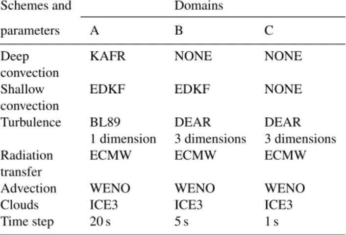
Figure 3a–c represent examples of the daytime profiles of air temperature, relative humidity, and horizontal wind speed. Examples of night profiles can be found in Fig. 3d–f. In general, the night-simulated profiles show slightly better accordance with model results.

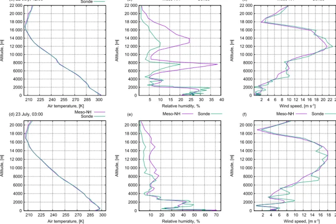
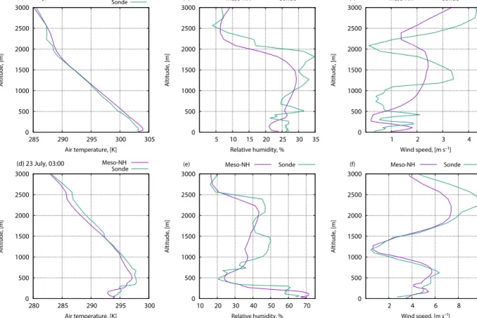
Figure 4 shows the same profiles, but for the lower tro-posphere level (3000 m altitude). Simulations are in good ac-cordance with observations. The simulation results are within

the confidence interval of the measurements as given by the radiosonde accuracy – ±0.5◦C, ±5 % relative humidity, and ±0.15 m s−1wind speed with 2σ confidence level (95.5 %).

The principal features of the profiles are well represented by the model. During daytime, air temperature and rela-tive humidity curves indicate that the model tends to rep-resent the height of the boundary layer at 2–2.5 km altitude well (around 2 km in Fig. 4a and b). Overall, Meso-NH re-produces the air temperature above the surface layer (over 500 m) very well. Near the surface, the Meso-NH tends to anticipate the development of the unstable boundary layer in the morning (09:00 and 12:00 UTC), simulating higher tem-peratures in the lower levels. In the late afternoon (18:00 and 21:00 UTC) the model also tends to anticipate the decrease in the temperature in the surface layer (see the Supplement, Fig. S1).

The vertical patterns of relative humidity and wind speed are good, as observed and modelled curves look similar; nev-ertheless simulations tend to be more conservative and their values do not represent all changes in altitude recorded by the radiosonde. Nocturnal low-level jets at the edge of the bound-ary layer are represented by the model, but their magnitude is slightly weaker than that observed. The complete set of ob-served versus simulated profiles can be found in the Supple-ment (Fig. S2). The moisture vertical profile in the boundary layer is well reproduced by the model, as can be seen in the graphs of the relative humidity (Figs. 4b, e, and S3). Above the boundary layer, the radiosondes show a dry layer, which is also well simulated. From 23 July the observations show the appearance of a moist layer close to the troposphere, the magnitude of which is overestimated by the model. At dawn on 24 July the radiosondes and the model indicate the ex-istence of a very moist layer close to the surface, with the formation of low clouds that were not formed in the simula-tions.

0 2000 4000 6000 8000 10 000 12 000 14 000 16 000 18 000 20 000 22 000 210 225 240 255 270 285 300 Altitude, [m ] Air temperature, [K] (a) 22 July, 12:00 Meso-NH_Sonde

0 2000 4000 6000 8000 10 000 12 000 14 000 16 000 18 000 20 000 22 000 5 10 15 20 25 30 35 40 Altitude, [m ] Relative humidity, % (b) Meso-NH Sonde 0 2000 4000 6000 8000 10 000 12 000 14 000 16 000 18 000 20 000 22 000 2 4 6 8 10 12 14 16 18 20 22 24 Altitude, [m ] Wind speed, [m s-1] (c) Meso-NH Sonde 0 2000 4000 6000 8000 10 000 12 000 14 000 16 000 18 000 20 000 210 225 240 255 270 285 300 Altitude, [m ] Air temperature, [K] (d) 23 July, 03:00 Meso-NH_Sonde

0 2000 4000 6000 8000 10 000 12 000 14 000 16 000 18 000 20 000 10 20 30 40 50 60 70 Altitude, [m ] Relative humidity, %

(e) Meso-NH Sonde

0 2000 4000 6000 8000 10 000 12 000 14 000 16 000 18 000 20 000 2 4 6 8 10 12 14 16 18 20 Altitude, [m ] (f) Meso-NH Sonde Wind speed, [m s-1_]

Figure 3. Examples of observed and simulated vertical profiles for 22 July at 12:00 UTC and 23 July at 03:00 UTC of air temperature (a, d), relative humidity (b, e), and wind speed (c, f).

Statistical results for them are the following: temperature average bias is −0.13◦C, RMSE is 1.49◦C, and the corre-lation coefficient is 0.99; relative humidity average bias is 0.59 %, RMSE is 11.26 %, and the correlation coefficient is 0.87; and for the wind speed average bias is 0.05 m s−1, RMSE is 2.07 m s−1, and the correlation coefficient is 0.90. These values testify that the simulation is in a good accor-dance with the observations, in line with similar studies of Meso-NH validation against radiosonde data (e.g. Masciadri et al., 2013).

5.2 Comparison with IPMA stations data

The model was also validated against 12 IPMA automatic meteorological stations. For this comparison the output of the bigger domain A was used. Geographical positions of the stations can be found in Fig. 1a. Scatter plots of air tempera-ture, relative humidity, and wind speed are shown in Fig. 5. It should be mentioned that not all stations provided the same set of variables. The scatter plots show the intercomparison of the model data (x axis) and the measured values (y axis) over all stations in the simulated period. The model tends to overestimate lower values of air temperature (14–24◦C) and slightly underestimate higher values (> 30◦C), as can be seen from Fig. 5a.

In some stations and for several times, the model simulates lower values of relative humidity within the range from 40 to 100 % (Fig. 5b). Figure 5c indicates that the wind speed is slightly underestimated by the model.

Statistical parameters (bias, mean absolute error, root mean square, and the correlation coefficient) for each station are shown in Table 2.

Simulated and observed air temperature are highly corre-lated (the correlation coefficient is higher that 0.91) with bias always less than 1◦. The worst results are observed in Por-talegre (square points in relative humidity plot in Fig. 5b), and a possible reason for this relies on the location of the station, which is installed in a complex mountain area, possi-ble not well represented in the model orography. Regarding wind speed, Meso-NH provides values for 10 m height while the measurements were made at 2 m. For proper compari-son modelled values were interpolated to the height of the sensors using a known logarithmic approach and a rough-ness length (which was also obtained from the model). Ta-ble 2 shows small biases, in general lower than 1 m s−1, and relatively high correlation coefficients for wind simula-tions (0.68–0.92). The lowest correlation coefficient is also obtained for Portalegre data. Overall, simulation results are in good agreement with synoptic station data, and the

0 500 1000 1500 2000 2500 3000 285 290 295 300 305 Altitude, [m ] Air temperature, [K] (a) 22 July, 12:00 Meso-NH

Sonde 0 500 1000 1500 2000 2500 3000 5 10 15 20 25 30 35 Altitude, [m ] Relative humidity, % (b) Meso-NH Sonde 0 500 1000 1500 2000 2500 3000 1 2 3 4 Altitude, [m ] Wind speed, [m s-1_] (c) Meso-NH Sonde 0 500 1000 1500 2000 2500 3000 280 285 290 295 300 Altitude, [m ] Air temperature, [K] (d) 23 July, 03:00 Meso-NH Sonde 0 500 1000 1500 2000 2500 3000 10 20 30 40 50 60 70 Altitude, [m ] Relative humidity, %

(e) Meso-NH Sonde

0 500 1000 1500 2000 2500 3000 2 4 6 8 10 Altitude, [m ] Wind speed, [m s-1_] (f) Meso-NH Sonde

Figure 4. Profiles of air temperature, relative humidity, and wind speed in low atmosphere on 22 July at 12:00 UTC and 23 July at 03:00 UTC.

12 14 16 18 20 22 24 26 28 30 32 34 36 38 40 12 14 16 18 20 22 24 26 28 30 32 34 36 38 40

Air temperature, Meso-NH, [

°C]

Air temperature, station, [°C] (a) Avis Beja Elvas Estremoz Evora Mertola Mora Portalegre Portel Reguengos Viana do Alentejo 20 30 40 50 60 70 80 90 100 20 30 40 50 60 70 80 90 100

Relative humidity, Meso-NH, %

Relative humidity, station, % (b) Avis Beja Elvas Mertola Portalegre Reguengos Viana do Alentejo 0 1 2 3 4 5 6 7 0 1 2 3 4 5 6 7 W in d sp ee d, M es o-N H , [ m s -1]

Wind speed, station, [m s-1_]

(c) Avis Beja Alvega Elvas Estremoz Evora Mertola Mora Portalegre Portel Reguengos Viana do Alentejo

Figure 5. Scatter plots of the comparison between Meso-NH simulation LAKE1 and measured values at synoptic stations. Air tempera-ture (a), relative humidity (b), and horizontal wind speed (c).

tical parameters are similar to other published works that use Meso-NH (e.g. Lascaux et al., 2013, 2015).

5.3 Comparison with data from the ALEX database In addition to the validation against the IPMA synoptic sta-tions, comparisons were made with data obtained at ALEX

meteorological stations (Barbosa, Cid Almeida, and Mon-tante platform). Their coordinates were used to locate cor-responding grid points on the C domain output. For land stations with grid points associated with water fraction, the nearest land grid point was chosen.

Figure 6 shows the time evolution of simulated and ob-served air temperature and wind speed at Cid Almeida,

16 18 20 22 24 26 28 30 32 34 36 38 Jul 21

12:00 Jul 2200:00 Jul 2212:00 Jul 2300:00 Jul 2312:00 Jul 2400:00 Jul 2412:00 Jul 2500:00

Air temperature, [

°C]

(a) Montante air temperature Meso-NH Measurements

0 1 2 3 4 5 6 7 8 Jul 21

12:00 Jul 2200:00 Jul 2212:00 Jul 2300:00 Jul 2312:00 Jul 2400:00 Jul 2412:00 Jul 2500:00

(d) Montante wind speed Meso-NH Measurements

14 16 18 20 22 24 26 28 30 32 34 36 38 Jul 21

12:00 Jul 2200:00 Jul 2212:00 Jul 2300:00 Jul 2312:00 Jul 2400:00 Jul 2412:00 Jul 2500:00

Air temperature, [

°C]

(b) Barbosa air temperature Meso-NH Measurements

0 1 2 3 4 5 6 Jul 21

12:00 Jul 2200:00 Jul 2212:00 Jul 2300:00 Jul 2312:00 Jul 2400:00 Jul 2412:00 Jul 2500:00

W in d sp ee d, [m s -1]

(e) Barbosa wind speed Meso-NH Measurements

16 18 20 22 24 26 28 30 32 34 36 38 Jul 21

12:00 Jul 2200:00 Jul 2212:00 Jul 2300:00 Jul 2312:00 Jul 2400:00 Jul 2412:00 Jul 2500:00

Air temperature, [

°C]

(c) Cid Almeida air temperature Meso-NH Measurements

0 1 2 3 4 5 6 7 8 Jul 21

12:00 Jul 2200:00 Jul 2212:00 Jul 2300:00 Jul 2312:00 Jul 2400:00 Jul 2412:00 Jul 2500:00

(f) Cid Almeida wind speed Meso-NH Measurements

W in d sp ee d, [m s -1] W in d sp ee d, [m s -1]

Figure 6. Observed and simulated air temperature and wind speed at 2 m for ALEX stations: Montante platform (a, d), Barbosa (b, e), and Cid Almeida (c, f) sites.

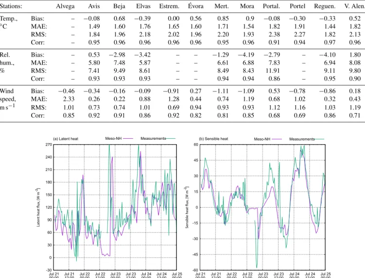
Table 2. Statistics for the hourly values of the station validation.

Stations: Alvega Avis Beja Elvas Estrem. Évora Mert. Mora Portal. Portel Reguen. V. Alen.

Temp., Bias: – −0.08 0.68 −0.39 0.00 0.56 0.85 0.9 −0.08 −0.30 −0.33 0.52 ◦ C MAE: – 1.49 1.60 1.76 1.65 1.60 1.71 1.54 1.82 1.91 1.44 1.82 RMS: – 1.84 1.96 2.18 2.02 1.96 2.20 1.93 2.38 2.27 1.82 2.13 Corr: – 0.95 0.96 0.96 0.96 0.96 0.95 0.96 0.91 0.94 0.97 0.96 Rel. Bias: – 0.53 −2.98 −3.42 – – −1.29 −4.19 −2.79 – −4.10 1.80 hum., MAE: – 5.80 7.48 5.87 – – 6.61 6.88 7.83 – 6.94 8.08 % RMS: – 7.41 9.49 8.61 – – 8.49 8.43 11.91 – 9.11 9.80 Corr: – 0.93 0.93 0.93 – – 0.94 0.94 0.86 – 0.95 0.90 Wind Bias: −0.46 −0.34 −0.16 −0.09 −0.91 0.27 −1.11 −1.09 0.53 −0.78 −0.86 0.18 speed, MAE: 2.33 0.26 0.22 0.88 1.28 0.44 0.74 1.19 0.68 1.02 0.32 0.43 m s−1 RMS: 1.01 0.73 0.74 1.01 0.69 0.94 0.93 0.93 1.12 1.16 1.03 1.19 Corr: 0.85 0.92 0.91 0.86 0.92 0.82 0.81 0.85 0.68 0.69 0.86 0.71 -30 0 30 60 90 120 150 180 210 240 270 Jul 21

00:00 Jul 2112:00 Jul 2200:00 Jul 2212:00 Jul 2300:00 Jul 2312:00 Jul 2400:00 Jul 2412:00 Jul 2500:00

Latent heat flux, [W m

-2]

(a) Latent heat Meso-NH Measurements

-60 -45 -30 -15 0 15 30 45 60 Jul 21

00:00 Jul 2112:00 Jul 2200:00 Jul 2212:00 Jul 2300:00 Jul 2312:00 Jul 2400:00 Jul 2412:00 Jul 2500:00

Sensible heat flux, [W m

-2]

(b) Sensible heat Meso-NH Measurements

Figure 7. Observed and simulated latent (a) and sensible (b) heat fluxes at Montante floating platform.

bosa, and Montante sites. Overall, the simulation results are slightly more conservative (except wind speed over the Montante platform), but in general, the patterns are well represented. The model could not represent the maximum and minimum temperatures well, especially in land stations where the temperature range is larger. Regarding wind speed, the model underestimates the maximum values at land sta-tions (Fig. 6e and f) and, on the contrary, overestimates the values at Montante platform (Fig. 6d), but the principal fea-tures of the curves are represented. Statistical values for this validation are as follows. For Barbosa, air temperature aver-age bias is 0.23◦C, RMSE is 1.37◦C and the correlation co-efficient is 0.98; for wind speed these values are as follows: average bias is 0.55 m s−1, RMSE is 1.08 m s−1, and the cor-relation coefficient is 0.73. For Cid Almeida, temperature av-erage bias is 0.5◦C, RMSE is 1.57◦C, and the correlation coefficient is 0.98, wind speed average bias is −0.36 m s−1, RMSE is 1.24 m s−1, and the correlation coefficient is 0.69.

For the Montante platform, air temperature average bias is −0.1◦C, RMSE is 1.22◦C, correlation is 0.98, wind speed average bias is −0.97 m s−1, RMSE is 1.55 m s−1, and the correlation coefficient is 0.61.

The temporal evolution of simulated and observed latent and sensible heat fluxes at Montante platform is shown in Fig. 7a and b. Overall patterns of the curves are similar but the simulated one is more smooth. Comparison demonstrates that for latent heat the RMSE is 57.34 W m−2with correla-tion coefficient of 0.47, and for sensible heat the RMSE is 13.39 W m−2with the correlation of 0.82.

Both observed and simulated curves of Fig. 7a reveal that sensible heat flux has two different periods during the day, positive when air-water temperature difference is negative, and vice versa, showing that during daytime the water re-ceives energy from the air and during nighttime the water warms the nearby air. The transition between the two regimes is well captured by the model. Figure 7b also shows that

0 90 180 270 360 Jul 21

12:00 Jul 2200:00 Jul 2212:00 Jul 2300:00 Jul 2312:00 Jul 2400:00 Jul 2412:00 Jul 2500:00

Wind direction, degrees

(a) Barbosa station Meso-NH Measurements

0 90 180 270 360 Jul 21

12:00 Jul 2200:00 Jul 2212:00 Jul 2300:00 Jul 2312:00 Jul 2400:00 Jul 2412:00 Jul 2500:00

Wind direction, degrees

(b) Cid Almeida station

Figure 8. Observed and simulated wind direction at Barbosa and Cid Almeida stations.

the magnitude of the sensible heat flux is relatively small when compared with the other terms of the energy balance. Daily maximum positive (negative) fluxes between 30 and 60 W m−2(−15 and −30 W m−2) are well reproduced by the model. An apparently strange behaviour appears on the after-noon of 22 July, with the sensible heat flux being almost zero. This effect, unfortunately not documented due to the lack of data, will be discussed later and is linked to the fact that the wind is very weak during this period (see Fig. 6d).

More detailed analysis of Fig. 7a shows that the lowest heat flux values usually occur during the afternoon (12:00– 18:00 UTC), under windless conditions, and high peaks in the early evening (20:00–21:00 UTC). The simulation repro-duces these peaks with 1–2 h delays that are related to the delay on the simulated wind speed. The magnitude of the la-tent heat flux daily maximum (order of 200–250 W m−2) is well captured by the model. The delay in the simulation of the peaks reduces the value of the correlation coefficient and is a manifestation of the so-called double-penalty that pe-nalize high-resolution model scores. As seen in Fig. 7b the simulated latent heat flux is almost zero between 14:00 and 16:00 UTC of 22 July. As pointed out before, there is a gap in the flux measurements during this period, but data from the day before indicate that the results are realistic. This effect of almost zero evaporation from water on a very hot day is contrary to common sense and will be discussed later.

Wind direction at ALEX stations is represented in Fig. 8. Different behaviour in wind direction between the two sta-tions from 21 to 23 July is clearly seen from measurement

data (green dots). In Barbosa station the wind changes from a north-west to a south regime during daytime while in Cid Almeida this effect is not observed. In the simulations this difference is not so clear, but is still visible during the after-noon on 22 July. Barbosa station, located on the north-west shore of the lake, indicates the presence of the lake breeze because its direction is the opposite to the dominant wind. At Cid Almeida station, on the south-east shore, the lake breeze is co-directed with the dominant wind.

6 Lake impact

To analyse the impact of the Alqueva reservoir on the lo-cal area the changes in the following atmospheric variables were considered: air temperature and potential temperature, relative humidity and water mixing ratio, and vertical and horizontal wind speed. In this section only B and C domain datasets were used.

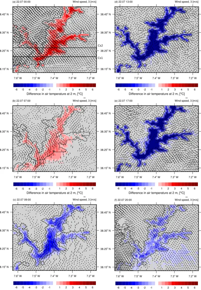
6.1 Impact on air temperature and relative humidity The lower layers of air are the first to be affected by the pres-ence of the water surface. Differpres-ences in air temperature at 2 m during 22 July are shown in Fig. 9, the warmest day of the IOP and thus with a stronger lake breeze. The posi-tive anomaly (up to 3–4◦C) can be traced during the period from 1 h after the sunset (21:00 UTC) to 1 h after the sun-rise (07:00 UTC). By positive and negative anomalies here we mean differences between LAKE1 and LAKE0

simula-Cs1 Cs2

Figure 9. Anomalies in air temperature at 2 m (in filled contours) and horizontal wind in LAKE1 experiment (arrays, the scale is indicated in the upper right corner of each figure) of the reservoir on 22 July 2014 in domain C. Horizontal lines in (a) indicate the location of cross sections Cs1 (southern) and Cs2 (northern).

(a) (b) (c) (d) (e) (f) 5 m s–1 5 m s–1 5 m s–1 _{5 m s}–1 5 m s–1 5 m s–1 2.5 m s–1 2.5 m s–1 2.5 m s–1 2.5 m s–1 2.5 m s–1 2.5 m s–1

Figure 10. East–west direction cross sections along 38.215◦N (Cs1, crosses the lake near Montante platform, Fig. 9a) of potential

temper-ature (filled contours) and wind vectors in the plane of the cross section (arrows), at different hours (indicated in the top of each figure) in the LAKE1 experiment at 250 m horizontal resolution. The wind vertical and horizontal scales are indicated in the upper right corner of each figure. The blue line on the surface level indicates the location of the reservoir.

tions. Examples of positive night anomalies are illustrated in Fig. 9a and b. Night north-west wind transports warm air from the lake to the south-east part of the reservoir for up to 2 km away from the shore. The daytime period is character-ized by negative temperature anomalies up to 7◦C (Fig. 9c– f). Initially, the effect is essentially limited by the lake bor-ders. When the large-scale sea breeze system arrives, tem-perature trace of the lake impact is advected by the wind and can be found in 10–12 km away from the south-east part of the reservoir (Fig. 9f).

Vertical cross sections help to illustrate the processes at different altitudes. Two different cross sections Cs1 and Cs2 are shown to provide a better visualization of the three-dimensional structure of air circulation above the lake. The first one crosses the lake near Montante platform and the

sec-ond in the middle, exact locations are indicated in Fig. 9a. Cross sections Cs1 along 38.215◦N (Fig. 10) show the evo-lution of wind and potential temperature during 22 July in the experiment with Alqueva (simulation LAKE1). The highest impact on the air temperature can be observed in the early af-ternoon (12:00–14:00 UTC). The boundary layer is cooling down and its height decreases from more than 2 km above the land outside to values close to 1 km over the lake sur-face (Fig. 10a). The thermal anomaly induced by the pres-ence of the reservoir seems to affect an area greater than what was identified at the surface, especially in the mid-dle of the boundary layer. Later on, at 19:00–20:00 UTC the powerful ocean breeze system reaches the area and cools the lower (1 km) layer of air by 6–7 K. The progression of the sea breeze front is impressively well shown in Fig. 10d

Figure 11. 2 m relative humidity anomalies (in filled contours) on 22 July 2014 in domain C.

(20:00 UTC), when it reaches the border of the reservoir, and in Fig. 10e and f (21:00–22:00 UTC), when it is already be-yond the east bank of the Alqueva reservoir. More cross

sec-tions of 22 July 2014 with potential temperature can be found in Fig. S4.

Alqueva causes a similar anomaly on 2 m relative humid-ity, which is shown in Fig. 11.

Figure 12. East–west direction cross sections Cs1 along 38.215◦N (a–c) and Cs2 along 38.274◦N (d–f) with the difference (LAKE1 minus LAKE0 simulations) of water mixing ratio (filled contours), and wind vectors in the plane of the cross section (arrows) in the LAKE1 experiment at 250 m horizontal resolution at different times (indicated in the top of each figure). The blue line on the surface level indicates the location of the reservoir.

At night when the temperature impact is negative some small negative differences in relative humidity can be seen over the lake surface (Fig. 11a). There are also traces of day-time positive impact, essentially due to the decrease in air temperature, advected by the sea breeze in the south-east di-rection. In the morning, however, the difference of relative humidity cannot be detected because the thermal impact is not strong enough (Fig. 11b). Figure 11c–e show how rel-ative humidity increases during the daytime over the water surface. The peak of the difference can reach 50 % in the

af-ternoon (Fig. 11f). In general, lake impact on relative humid-ity is limited by the area of the reservoir and does not spread over the surrounding land.

6.2 Breeze effects

Differences in near-surface sensible heat fluxes and contrast of the air temperature over the land and water surfaces during the daytime induce the formation of the lake breeze system. The development of the lake breeze is illustrated in Fig. 9 (ar-rows that correspond to the wind speed lesser than 0.5 m s−1

3 4 5 6 7 8 9 10 11 12 Jul 21

12:00 Jul 2200:00 Jul 2212:00 Jul 2300:00 Jul 2312:00 Jul 2400:00 Jul 2412:00 Jul 2500:00

Water vapour mixing ratio, [g kg

]

-1

Measurements Meso-NH

Figure 13. Observed and simulated water vapour mixing ratio at the Montante platform.

are not plotted). During the night, the large-scale circulation (Fig. 9a and b) is dominant in the area. After the sunrise (07:00–08:00 UTC) the air temperature over the water face becomes lower than the air temperature over the sur-rounding areas, which induce a thermal circulation directed from the centre of the lake to its shores. The breeze intensifies during the afternoon reaching 6 m s−1in some areas (Fig. 9d and e).

Daytime cross sections Cs1 in Fig. 10a–c indicate that the direct lake breeze can be found on altitudes up to 300 m above the lake, with a divergent flow over the water sur-face. The lake breeze intensity and pattern depends on the local orography, but usually the traces can be found 4–6 km away from the lake shores (Fig. 10c). In altitude, a return flow is visible in the eastward wind component over the west shore and a westward component in the east of the reservoir, which causes an upper-level convergence that can be seen in Fig. 10a–c. This will be discuss together with the effects of the reservoir on the moisture field, in which the structure of the lake breeze system is more visible.

In the late afternoon (18:00 UTC) the negative temperature anomaly due to the presence of the lake is getting weaker, and the breeze system starts to wane and dissipate. At 19:00– 20:00 UTC the ocean breeze arrives to the area and overlaps the local circulations (Fig. 10d–f).

Cross sections Cs1 and Cs2 presented in Fig. 12 show that the lake breeze system includes a descending branch over the reservoir that carries dry air from a height of about 2– 2.5 km and redistributes it over the lake surface. Additional cross sections illustrating this process can be found in the Supplement (Figs. S5 and S6).

This dry downstream is confirmed by the measurements of water vapour mixing ratio at the Montante platform. As can be seen in Fig. 13 the observed and the simulated mixing ratio of water vapour have a daily minimum with average

val-ues of about 8–8.5 g kg−1around 14:00–16:00 UTC. During the afternoon of 22 July, the day with a strong lake breeze, the minimum reached a value lower than 6 g kg−1. Out of the period in which the air over the lake subsides, the water vapour mixing ratio returns back to 9–10.5 g kg−1. The pres-ence of this dry downstream was proposed as a hypothesis by Potes et al. (2017) and is proved through the performed sim-ulations. In the same figure it is clearly seen that the model tends to overestimate the mixing ratio, except during the af-ternoon of 22 July.

However, Fig. 12 also shows that outside the reservoir there are zones of low-level convergence and upward motion that increase the moisture of the boundary layer and form some kind of lake breeze fronts. The complex shape of the reservoir implies also an complex 3-D structure of the breeze system. Towards the southernmost part, near the dam, the low-level divergent breeze circulation is very clear, but the convergence upper-level return current is weaker (Fig. 12a– c). In contrast, near the middle of the reservoir (cross sec-tion Cs2 in Fig. 12d–f) where two water branches exist, the circulation near the surface is more complex due to the presence of a land area in between, but the subsidence mo-tion is more prominent, inducing a decrease in mixing ratio through the boundary layer, which reaches a magnitude of about 4 g kg−1at 16:00 UTC (Fig. 12f).

Figure 14 illustrates this process in a horizontal plane. At midnight (Fig. 14b) the reservoir does not directly af-fect vapour mixing ratio in the air. In the morning hours, when the sun rises, but the breeze system is not yet formed, a positive impact on the moisture over the lake can be seen due to the increase in the evaporation. This anomaly affects the air above the central and southern parts of the reservoir and is advected to nearby areas (Fig. 14c). Later in the af-ternoon, with the formation of the lake breeze, a negative impact can be traced over the water surface due to the de-scending branches of the local circulation (Fig. 14d and e). This explains the afternoon decrease in the water vapour mixing ratio observed at the Montante platform, as seen in Fig. 13. The localization of the area of this negative anomaly changes in time, but predominantly it is over the larger south-ern part of the reservoir. With the dissipation of the local lake breeze system and the arrival of the stronger large-scale north-western wind, the negative moisture anomaly over the reservoir disappears and a positive effect is visible in the downwind region (Fig. 14a and f), due to the increase in evaporation (note that Fig. 14a corresponds to the night of 21 to 22 July, when the effect was more noticeable).

During daytime, water temperature is lower than air tem-perature, which is associated with a very weak air circula-tion over the water surface, which leads to very low evapo-ration from the lake (refer to low latent heat flux values in Fig. 7a). This period of day is characterized by higher evapo-ration over the land than over water. By late afternoon when the dominant sea breeze system reaches the region, the north-western wind accelerates significantly when passing over the

Figure 14. Observed and simulated water vapour mixing ratio anomalies in filled contours on 22 July 2014 in domain C for selected hours.

smooth surface of the lake. As result, evaporation from the lake becomes very intense.

7 Conclusions

In this work the authors studied the formation and magnitude of the summer lake breeze in the Alqueva reservoir, southern Portugal, and its impacts on local weather. The study was based on Meso-NH simulations of a well documented case

study of 22–24 July 2014. This period was used for several reasons. First, a large volume of meteorological data was col-lected during these days, which allowed for a validation of the simulation results. Secondly, this period was hot and dry, which is typical for most summer days in the region.

The model allowed simulations with horizontal resolution of 250 m, which is fine enough to resolve such relatively small-scale lake breeze and to spot the impact of the reser-voir on the detailed local boundary layer structure. Due to the “youth” of the Alqueva reservoir it is possible to run an atmospheric model with the surface conditions prevailing be-fore the filling of the reservoir. Two simulations, one with Alqueva and another one without it, allow the raw impact of the lake on the local weather regime to be evaluated.

Formation and dissipation of the daytime breeze system induced by the reservoir are described in the work. On hot summer mornings the difference between air tempera-tures above water and neighbouring land surfaces induces the radial movement of air from the lake. The breeze sys-tem starts to form in the morning and the peak of the wind speed reaches 6 m s−1during the afternoon. Simulation re-sults show that the lake breeze could be detected at a distance of more than 6 km away from the shores and on altitudes up to 300 m above the water surface. In late afternoon the dis-sipation stage of the lake breeze system is anticipated with the arrival of the larger-scale sea breeze from the Portuguese west Atlantic coast. In early evening (19:00–20:00 UTC) the local lake breeze system cannot be detected anymore. No re-verse land breeze is detected during the night.

Lake breeze system brings dry air from upper atmospheric layers (2–2.5 km) to near-surface levels above the reservoir. This effect leads to the fact that the air above the surface of the lake becomes more dry in terms of water vapour mixing ratio, in spite of the fact that its relative humidity can increase up to 50 % due to the decrease in air temperature.

The simulations testify to the observed very low evapora-tion from water surface during the daytime (0–120 W m−2in terms of latent heat flux), due to weak winds and the sta-ble stratification of the internal atmospheric surface layer. At nighttime, the strong wind associated with the peninsu-lar peninsu-larger-scale circulation induced by the sea–land contrasts, originates a very high evaporation rate (200–250 W m−2).

The cooling effect of the reservoir can decrease the air temperature by up to 7◦C; nevertheless it is limited by the lake borders and normally cannot be seen farther than few kilometres away from the shore, mostly in the south-east di-rection. The cooling can be found up to 1200 m above the lake surface.

Further work suggests two options: first, tuning the lake model and its initialization in order to obtain more accu-rate results and reduce validation biases; second, carry out a longer experiment, which would cover a 12-month period. Such a simulation could reveal seasonal aspects of the impact of Alqueva on local weather.

Data availability. Data obtained during the ALEX 2014

obser-vational experiment and used here are available via http://www. alex2014.cge.uevora.pt/data/ (Salgado, 2018).

The Supplement related to this article is available online at https://doi.org/10.5194/hess-22-5191-2018-supplement.

Author contributions. The three authors conceptualized the study.

MI and RS performed the Meso-NH simulations and the exploita-tion of its results. MP prepared the measured data and assisted in its use. MI wrote the first draft manuscript. All the three authors contributed to the analysis, interpretation and writing.

Competing interests. The authors declare that they have no conflict

of interest.

Special issue statement. This article is part of the special

is-sue “Modelling lakes in the climate system (GMD/HESS inter-journal SI)”. It is a result of the 5th workshop on “Parameterization of Lakes in Numerical Weather Prediction and Climate Modelling”, Berlin, Germany, 16–19 October 2017.

Acknowledgements. The work is co-funded by the European Union

through the European Regional Development Fund, included in COMPETE 2020 (Operational Program Competitiveness and Inter-nationalization) through the ICT project (UID/GEO/04683/2013) with the reference POCI-01-0145-FEDER-007690 and also through the ALOP project (ALT20-03-0145-FEDER-000004). Experiments were accomplished during the field campaign funded by FCT and FEDER-COMPETE: ALEX (EXPL/GEO-MET/1422/2013) FCOMP-01-0124-FEDER-041840.

Edited by: Wim Thiery

Reviewed by: two anonymous referees

References

Bates, G. T., Giorgi, F., and Hostetler, S. W.: Toward the Simula-tion of the Effects of the Great Lakes on Regional Climate, Mon. Weather Rev., 121, 1373–1387, https://doi.org/10.1175/1520-0493(1993)121<1373:TTSOTE>2.0.CO;2, 1993.

Bechtold, P., Bazile, E., Guichard, F., Mascart, P., and Richard,

E.: A mass-flux convection scheme for regional and

global models, Q. J. Roy. Meteorol. Soc., 127, 869–886, https://doi.org/10.1002/qj.49712757309, 2001.

Bischoff-Gauß, I., Kalthoff, N., and Fiebig-Wittmaack, M.: The influence of a storage lake in the Arid Elqui Valley in Chile on local climate, Theor. Appl. Climatol., 85, 227–241, https://doi.org/10.1007/s00704-005-0190-8, 2006.

Bonan, G. B.: Sensitivity of a GCM Simulation

Cli-mate, 8, 2691–2704, https://doi.org/10.1175/1520-0442(1995)008<2691:SOAGST>2.0.CO;2, 1995.

Bougeault, P. and Lacarrere, P.: Parameterization of Orography-Induced Turbulence in a Mesobeta–Scale Model, Mon. Weather Rev., 117, 1872–1890, https://doi.org/10.1175/1520-0493(1989)117<1872:POOITI>2.0.CO;2, 1989.

Cohard, J. M. and Pinty, J. P.: A comprehensive two-moment warm microphysical bulk scheme. I: Description and tests, Q. J. Roy. Meteorol. Soc., 126, 1815–1842, https://doi.org/10.1002/qj.49712656613, 2000.

Cotton, W. R. and Pielke, R. A. S.: Human Impacts on Weather and Climate, 2nd Edn., Cambridge University Press, Cambridge, 2007.

Crosman, E. T. and Horel, J. D.: Idealized Large-Eddy Simula-tions of Sea and Lake Breezes: Sensitivity to Lake Diameter, Heat Flux and Stability, Bound.-Lay. Meteorol., 144, 309–328, https://doi.org/10.1007/s10546-012-9721-x, 2012.

Cuxart, J., Bougeault, P., and Redelsperger, J.-L.: A tur-bulence scheme allowing for mesoscale and large-eddy

simulations, Q. J. Roy. Meteorol. Soc., 126, 1–30,

https://doi.org/10.1002/qj.49712656202, 2000.

Drobinski, P. and Dubos, T.: Linear breeze scaling: from large-scale land/sea breezes to mesoscale inland breezes, Q. J. Roy. Meteo-rol. Soc., 135, 1766–1775, https://doi.org/10.1002/qj.496, 2009. Ekhtiari, N., Grossman-Clarke, S., Koch, H., Meira de Souza, W., Donner, R. V., and Volkholz, J.: Effects of the Lake Sobradinho Reservoir (Northeastern Brazil) on the Regional Climate, Cli-mate, 5, 50, https://doi.org/10.3390/cli5030050, 2017.

Faroux, S., Kaptué Tchuenté, A. T., Roujean, J. L., Masson, V., Mar-tin, E., and Le Moigne, P.: ECOCLIMAP-II/Europe: a twofold database of ecosystems and surface parameters at 1 km resolu-tion based on satellite informaresolu-tion for use in land surface, mete-orological and climate models, Geosci. Model Dev., 6, 563–582, https://doi.org/10.5194/gmd-6-563-2013, 2013.

Fouquart, Y. and Bonnel, B.: Computations of Solar Heating of the Earth’s Atmosphere – A New Parameterization, Beitr. Phys. At-mos., 53, 35–62, 1980.

Hartmann, D. L.: Global physical climatology, Int. Geophys., Else-vier Science, 498 pp., 1994.

Hoinka, K. P. and Castro, M. D.: The Iberian Peninsula thermal low, Q. J. Roy. Meteorol. Soc., 129, 1491–1511, 2003.

Jarvis, A., Guevara, E., Reuter, H. I., and Nelson, A. D.: Hole – filled SRTM for the globe: version 4: data grid, CGIAR-CSI, Washington, USA, 19 August 2008.

Kain, J. S. and Fritsch, M. J.: A One-Dimensional

Entraining/Detraining Plume Model and Its

Appli-cation in Convective Parameterization, J. Atmos.

Sci., 47, 2784–2802,

https://doi.org/10.1175/1520-0469(1990)047<2784:AODEPM>2.0.CO;2, 1990.

Lac, C., Chaboureau, J.-P., Masson, V., Pinty, J.-P., Tulet, P., Es-cobar, J., Leriche, M., Barthe, C., Aouizerats, B., Augros, C., Aumond, P., Auguste, F., Bechtold, P., Berthet, S., Bielli, S., Bosseur, F., Caumont, O., Cohard, J.-M., Colin, J., Couvreux, F., Cuxart, J., Delautier, G., Dauhut, T., Ducrocq, V., Filippi, J.-B., Gazen, D., Geoffroy, O., Gheusi, F., Honnert, R., Lafore, J.-P., Lebeaupin Brossier, C., Libois, Q., Lunet, T., Mari, C., Maric, T., Mascart, P., Mogé, M., Molinié, G., Nuissier, O., Pan-tillon, F., Peyrillé, P., Pergaud, J., Perraud, E., Pianezze, J., Re-delsperger, J.-L., Ricard, D., Richard, E., Riette, S., Rodier, Q.,

Schoetter, R., Seyfried, L., Stein, J., Suhre, K., Taufour, M., Thouron, O., Turner, S., Verrelle, A., Vié, B., Visentin, F., Vion-net, V., and Wautelet, P.: Overview of the Meso-NH model ver-sion 5.4 and its applications, Geosci. Model Dev., 11, 1929– 1969, https://doi.org/10.5194/gmd-11-1929-2018, 2018. Lascaux, F., Masciadri, E., and Fini, L.: MOSE: operational forecast

of the optical turbulence and atmospheric parameters at Euro-pean Southern Observatory ground-based sites – II. Atmospheric parameters in the surface layer 0–30 m, Mon. Notic. Roy. Astron. Soc., 436, 3147–3166, https://doi.org/10.1093/mnras/stt1803, 2013.

Lascaux, F., Masciadri, E., and Fini, L.: Forecast of surface layer meteorological parameters at Cerro Paranal with a mesoscale at-mospherical model, Mon. Notic. Roy. Astron. Soc., 449, 1664– 1678, https://doi.org/10.1093/mnras/stv332, 2015.

Lee, X., Liu, S., Xiao, W., Wang, W., Gao, Z., Cao, C., Hu, C., Hu, Z., Shen, S., Wang, Y., Wen, X., Xiao, Q., Xu, J., Yang, J., and Zhang, M.: The Taihu Eddy Flux Network: An Obser-vational Program on Energy, Water, and Greenhouse Gas Fluxes of a Large Freshwater Lake, B. Am. Meteorol. Soc., 95, 1583– 1594, https://doi.org/10.1175/BAMS-D-13-00136.1, 2014. Lin, Z., Jiming, J., Shih-Yu, W., and Ek, M. B.: Integration of

remote-sensing data with WRF to improve lake-effect precipi-tation simulations over the Great Lakes region, J. Geophys. Res.-Atmos., 117, d09102, https://doi.org/10.1029/2011JD016979, 2012.

Lopes, F., Silva, H. G., Salgado, R., Potes, M., Nicoll, K. A., and Harrison, R. G.: Atmospheric electrical field measurements near a fresh water reservoir and the formation of the lake breeze, Tellus A, 68, 31592, https://doi.org/10.3402/tellusa.v68.31592, 2016.

Lunet, L., Lac, C., Auguste, F., Visentin, F., Masson, V., and Es-cobar, J.: Combination of WENO and Explicit Runge–Kutta Methods for Wind Transport in the Meso-NH Model, Mon. Weather Rev., 145, 3817–3838, https://doi.org/10.1175/MWR-D-16-0343.1, 2017.

Masciadri, E., Lascaux, F., and Fini, L.: MOSE: operational forecast of the optical turbulence and atmospheric parame-ters at European Southern Observatory ground-based sites – I. Overview and vertical stratification of atmospheric parame-ters at 0–20 km, Mon. Notic. Roy. Astron. Soc., 436, 1968–1985, https://doi.org/10.1093/mnras/stt1708, 2013.

Masson, V.: A Physically-Based Scheme For The Urban Energy Budget In Atmospheric Models, Bound.-Lay. Meteorol., 94, 357–397, https://doi.org/10.1023/A:1002463829265, 2000. Masson, V., Le Moigne, P., Martin, E., Faroux, S., Alias, A.,

Alkama, R., Belamari, S., Barbu, A., Boone, A., Bouyssel, F., Brousseau, P., Brun, E., Calvet, J.-C., Carrer, D., Decharme, B., Delire, C., Donier, S., Essaouini, K., Gibelin, A.-L., Giordani, H., Habets, F., Jidane, M., Kerdraon, G., Kourzeneva, E., Lafaysse, M., Lafont, S., Lebeaupin Brossier, C., Lemonsu, A., Mahfouf, J.-F., Marguinaud, P., Mokhtari, M., Morin, S., Pigeon, G., Sal-gado, R., Seity, Y., Taillefer, F., Tanguy, G., Tulet, P., Vincendon, B., Vionnet, V., and Voldoire, A.: The SURFEXv7.2 land and ocean surface platform for coupled or offline simulation of earth surface variables and fluxes, Geosci. Model Dev., 6, 929–960, https://doi.org/10.5194/gmd-6-929-2013, 2013.

Miranda, P. M. A., Abreu, F., and Salgado, R.: Estudo de Impacte Ambiental do Alqueva, Tech. rep., Instituto de ciencia aplicada e

tecnologia, Faculdade de Ciências, Universidade de Lisboa, Lis-boa, 1995.

Miranda, P. M. and James, I. N.: Non-linear three-dimensional ef-fects on gravity-wave drag: Splitting flow and breaking waves, Q. J. Roy. Meteorol. Soc., 118, 1057–1081, 1992.

Mironov, D.: Parameterization of lakes in numerical weather pre-diction, Description of a lake model, COSMO Technical Report, Deutscher Wetterdienst, Offenbach am Main, 41 pp., 2008. Morcrette, J. J.: Radiation and cloud radiative properties in

the European Centre for Medium Range Weather Forecasts forecasting system, J. Geophys. Res.-Atmos., 96, 9121–9132, https://doi.org/10.1029/89JD01597, 1991.

Nicoll, K. A., Harrison, R. G., Silva, H. G., Salgado, R., Melgâo, M., and Bortoli, D.: Electrical sensing of the dynamical struc-ture of the planetary boundary layer, Atmos. Res., 202, 81–95, https://doi.org/10.1016/j.atmosres.2017.11.009, 2018.

Noilhan, J. and Mahfouf, J. F.: The ISBA land surface pa-rameterisation scheme, Global Planet. Change, 13, 145–159, https://doi.org/10.1016/0921-8181(95)00043-7, 1996.

Pergaud, J., Masson, V., Malardel, S., and Couvreux, F.: A Param-eterization of Dry Thermals and Shallow Cumuli for Mesoscale Numerical Weather Prediction, Bound.-Lay. Meteorol., 132, 83– 106, https://doi.org/10.1007/s10546-009-9388-0, 2009. Pielke Sr., R. A.: A Three-Dimensional Numerical Model

of the Sea Breezes Over South Florida, Mon. Weather

Rev., 102, 115–139,

https://doi.org/10.1175/1520-0493(1974)102<0115:ATDNMO>2.0.CO;2, 1974.

Pielke Sr., R. A.: Mesoscale Meteorological Modeling, 3rd Edn., Academic Press, 760, 2013.

Pinty, J. P. and Jabouille, P.: A mixed-phase cloud parameteriza-tion for use in mesoscale non-hydrostatic model: simulaparameteriza-tions of a squall line and of orographic precipitations, in: Proc. Conf. of Cloud Physics, Everett, WA, USA, 217–220, 1998.

Policarpo, C., Salgado, R., and Costa, M. J.: Numerical Simulations of Fog Events in Southern Portugal, Adv. Meteorol., 2017, 16 pp., 2017.

Potes, M., Salgado, R., Costa, M. J., Morais, M.,

Bor-toli, D., Kostadinov, I., and Mammarella, I.: Lake–

atmosphere interactions at Alqueva reservoir: a case

study in the summer of 2014, Tellus A, 69, 1272787, https://doi.org/10.1080/16000870.2016.1272787, 2017.

Salgado, R.: Interacção solo-atmosfera em clima semi-àrido, PhD thesis, Universidade de Èvora, Èvora, 2006.

Salgado, R. and Le Moigne, P.: Coupling of the FLake model to the Surfex externalized surface model, Boreal Environ. Res., 15, 231–244, 2010.

Salgado, R., Miranda, P. M. A., Lacarrère, P., and

Noil-han, J.: Boundary layer development and summer

circulation in Southern Portugal, Tethys, 12, 33–44,

https://doi.org/10.3369/tethys.2015.12.03, 2015.

Salgado, R., Potes, M., Albino, A., Apolinário, J., Barbosa, S., Bárias, S., Beliche, P., Bortoli, D., Canhoto, P., Costa, M. J., Fernandes, R. M., Harrison, G., Ilhéu, A., Le Moigne, P., Lima, R., Lopes, F., Lopes, T., Marques, J., Melgão, M., Miranda, P. M., Morais, M., Murteira, M., Nicoll, K., No-vais, M. H., Parrondo, M. C., Pereira, S., Policarpo, C., Prior, V., Rodrigues, C. M., Rosado, J., Sá, A., Serafim, A., Silva, H., Soares, P. M. M., Tlemçani, M., and Zavattieri, A.: The ALEX2014 Alqueva hydro-meteorological database, available at: http://www.alex2014.cge.uevora.pt/data/, last access: 3 Octo-ber 2018.

Samuelsson, P., Kourzeneva, E., and Mironov, D.: The impact of lakes on the European climate as simulated by a regional climate model, Boreal Environ. Res., 15, 113–129, 2006.

Segal, M., Leuthold, M., Arritt, R. W., Anderson, C., and

Shen, J.: Small Lake Daytime Breezes: Some

Obser-vational and Conceptual Evaluations, B. Am.

Meteo-rol. Soc., 78, 1135–1147,

https://doi.org/10.1175/1520-0477(1997)078<1135:SLDBSO>2.0.CO;2, 1997.

Silva, A., De Lima, I., Santo, F. E., and Pires, V.: Assessing changes in drought and wetness episodes in drainage basins using the Standardized Precipitation Index, Bodenkultur, 65, 31–37, 2014. Stein, J., Richard, E., Lafore, J. P., Pinty, J. P., Asencio, N., and Cosma, S.: High-Resolution Non-Hydrostatic Simu-lations of Flash-Flood Episodes with Grid-Nesting and Ice-Phase Parameterization, Meteorol. Atmos. Phys., 72, 203–221, https://doi.org/10.1007/s007030050016, 2000.

Thiery, W., Martynov, A., Darchambeau, F., Descy, J.-P., Plisnier, P.-D., Sushama, L., and van Lipzig, N. P. M.: Understanding the performance of the FLake model over two African Great Lakes, Geosci. Model Dev., 7, 317–337, https://doi.org/10.5194/gmd-7-317-2014, 2014.