Dataset morphing to analyze the performance of recommender systems

(1)

FACULDADE DE

ENGENHARIA DA

UNIVERSIDADE DO

PORTO

Dataset morphing to analyze the

performance of recommender systems

André Gomes Ferreira Araújo Correia

Mestrado Integrado em Engenharia Informática e Computação Supervisor: Carlos Manuel Milheiro de Oliveira Pinto Soares

Co-Supervisor: Alípio Mário Guedes Jorge

(2)

c

(3)

Dataset morphing to analyze the performance of

recommender systems

André Gomes Ferreira Araújo Correia

Mestrado Integrado em Engenharia Informática e Computação

Approved in oral examination by the committee:

Chair: Rui Carlos Camacho de Sousa Ferreira da Silva External Examiner: Pavel Bernard Brazdil

Supervisor: Carlos Manuel Milheiro de Oliveira Pinto Soares

(4)

(5)

Abstract

Recommender Systems analyze patterns of user interest in items to provide personalized sug-gestions that suit a user’s preference. Therefore, they have become fundamental applications in electronic commerce and information access in such a way that today Recommender Systems are an accepted technology used by market leaders in several industries. One of the most successful techniques for Recommender Systems, called Collaborative Filtering, has been developed and im-proved over the last few years to the point where a wide variety of algorithms exist for generating recommendations. Thus, clearly identifying the best algorithm for a given purpose has proven challenging. Different algorithms may be better or worse on different datasets and theoretical knowledge about the performance of those algorithms is missing. Even the empirical research that has taken place produced non-generalizable results, due to the absence of a large number of datasets. Furthermore, in real world Recommender Systems, it is reasonable to approach ratings data as a data stream: ratings are continuously being generated. Thus, as data changes, the best algorithm may change as well. This dissertation aims for a better understanding of algorithm be-havior. The main goal is to develop a methodology to systematically manipulate real datasets, to support the identification of reliable relationships between algorithm performance and data char-acteristics. It consists of the iterative application of transformations (morphing) on real datasets which represent an interesting behavior of algorithms (e.g., algorithm A is better than B on one dataset but the opposite happens in the other). Therefore, the proposed methodology can be used to understand the strengths and weaknesses of algorithms. In the experiments carried out, the proposed methodology was used to select Collaborative Filtering algorithms on the scope of item recommendation problem. Each algorithm was trained on a collection of real-world datasets and evaluated on a set of suitable metrics. The algorithm selection problem was formulated as a classi-fication task, where the target attribute is the best algorithm according to each performance metric. The results show that the proposed approach is viable and that the metafeatures considered contain information that is useful to predict the best algorithm for a dataset.

Keywords: Recommender Systems, Collaborative Filtering, Metalearning, Algorithm selec-tion.

(6)

(7)

Resumo

Os Sistemas de Recomendação analisam padrões nos gostos dos utilizadores, por forma a sug-erirem produtos que vão ao encontro das suas preferências. Desempenhando atualmente um papel fundamental, no que ao comércio eletrónico diz respeito, os Sistemas de Recomendação tornaram-se uma tecnologia aceite e utilizada pelos principais líderes de mercado em muitas indústrias. Uma das técnicas de Sistemas de Recomendação com maior sucesso, chamada Collaborative Filtering, dispõe hoje de um vasto leque de algoritmos de recomendação, tal a forma como foi desenvolvida e aprimorada ao longo dos últimos anos. Como tal, a escolha do melhor algoritmo, para um de-terminado problema, representa um enorme desafio. Não obstante, diferentes algoritmos poderem apresentar melhor ou pior desempenho dependendo do problema, o conhecimento teórico sobre o desempenho dos mesmos é escasso. Mesmo os estudos empíricos realizados, produziram resulta-dos cuja generalização não é possível, dada a inexistência de um vasto e diversificado número de conjunto de dados. Acresce que, em Sistemas de Recomendação reais, é razoável considerar os dados como sendo um fluxo, uma vez que novos ratings estão permanentemente a ser gerados ou alterados. Ora, um bom Sistema de Recomendação deve ter em consideração as constantes alter-ações nos dados, adoptando as devidas medidas por forma a garantir que o algoritmo utilizado é sempre o mais adequado. Esta dissertação visa contribuir para a melhoria do conhecimento sobre o comportamento dos algoritmos. O principal objectivo passa por desenvolver uma metodologia que, de forma sistemática, permita manipular conjunto de dados reais, tendo em vista a identifi-cação de uma relação fidedigna entre o desempenho dos algoritmos e as características dos dados. Tal metodologia consiste na aplicação iterativa de operações de transformação (morphing) em conjuntos de dados reais, para os quais algoritmos de recomendação apresentem comportamentos particularmente interessantes (por exemplo, o algoritmo A ser melhor do que o algoritmo B num determinado conjunto de dados, e o seu contrário num outro determinado conjunto de dados). A metodologia proposta pode assim ser utilizada para perceber os pontos fortes e as debilidades de um determinado algoritmo. Nas experiências realizadas no decurso desta dissertação, a metodolo-gia proposta foi utilizada tendo em vista a seleção de algoritmos Collaborative Filtering. Cada algoritmo foi treinado num leque de conjuntos de dados reais e o seu desempenho foi avaliado à luz de um conjunto de métricas aplicáveis. O problema da seleção do algoritmo foi formulado como um problema de classificação, em que a variável objetivo representa o melhor algoritmo, de acordo com determinada métrica. Os resultados demonstram, não apenas que a metodologia proposta é viável, mas que as meta características utilizadas contém informação útil para prever qual o melhor algoritmo para um determinado conjunto de dados.

(8)

(9)

Acknowledgements

Firstly, I would like to thank my supervisors, Carlos Soares and Alípio Jorge, for guiding me throughout this dissertation and pointing me in the right directions. I’m very thankful for your patience and provided expertise. Thank you for all the questions answered, for the constant moti-vation and for always believing in this work even when it was so hard.

I would also like to thank Tiago Cunha, from INESC TEC, for his valuable insights and kind availability to help me.

A sincere thank you to all my friends, colleagues and teachers who worked with me and helped me throughout my academic path.

A special word of love to Joana, for being the brightest light in my life. A work of this dimension is only possible due to her support, patience and love.

Lastly, but most importantly, I would like to thank my mom and dad for always believing in me and for assuring me that no matter what, they would always stay by my side.

This work is funded by ERDF through the Operational Programme of Competitiveness and Internationalization — COMPETE 2020 — of Portugal 2020 within project PushNews | POCI-01-0247-FEDER-0024257.

(10)

(11)

“An investment in knowledge pays the best interest”

(12)

(13)

1.2 Research Questions . . . 3 1.3 Document Structure . . . 5 2 Background 7 2.1 Recommender Systems . . . 7 2.1.1 Definition . . . 7 2.1.2 Algorithmic approaches . . . 9 2.1.3 Evaluation . . . 13 2.2 Metalearning . . . 17 2.2.1 Definition . . . 18 2.2.2 Metafeatures . . . 19 2.2.3 Algorithmic approaches . . . 20

2.3 Metalearning for Recommender Systems . . . 21

3 Morphing Recommendation Datasets 23 3.1 Dataset Morphing . . . 24

3.2 Dataset Footprints: analyzing algorithm behavior using Dataset Morphing . . . . 26

3.3 Discussion . . . 28

3.3.1 Source and target dataset selection criteria . . . 28

3.3.2 Properties of performance . . . 28 3.3.3 Dataset transformations . . . 29 3.3.4 Application scope . . . 30 4 Empirical Evaluation 31 4.1 Base-level setup . . . 32 4.2 Data . . . 33

4.3 Dataset transformations setup . . . 35

4.4 Metafeatures . . . 36

4.5 Meta-level setup . . . 38

5 Experimental Results 41 5.1 Base-level results . . . 41

5.2 Meta-level results . . . 42

5.2.1 Relationship between metafeatures and algorithm performance . . . 44

5.2.2 Intra-domain algorithm performance prediction . . . 46

(14)

CONTENTS

5.2.4 Trajectories vs random samples . . . 54

5.3 Meta-knowledge . . . 57

6 Conclusions and Future Work 67 6.1 Answer Research Questions . . . 68

6.2 Limitations . . . 70 6.3 Main Contributions . . . 70 6.4 Future Work . . . 70 References 73 A Base-level results 77 A.1 Recall . . . 77

A.2 Column-wise transformations . . . 77

B Meta-level results 85 B.1 Metafeatures . . . 85

(15)

List of Figures

1.1 Transfer of (meta)knowledge across samples of the same meta-dataset. . . 4

1.2 Transfer of (meta)knowledge across samples of different meta-datasets. . . 4

2.1 Area Under the ROC-curve (AUC). . . 17

3.1 Initial datasets — source dataset (Ds) and target dataset (Dt). . . 25

3.2 Datasets transformations. . . 26

3.3 Experimental framework. . . 27

4.1 Source (Ds) and target (Dt) datasets selection: subset the same dataset D. . . 34

4.2 Source (Ds) and target (Dt) datasets selection: subset different D1and D2datasets. 34 4.3 Source (Ds) and target (Dt) datasets pairing. . . 35

4.4 Row-wise dataset transformations process. . . 35

4.5 Multiple trajectories possible between source (Ds) and target (Dt) datasets. . . 36

4.6 Framework for systematic development of metafeatures [PSMM16]. . . 37

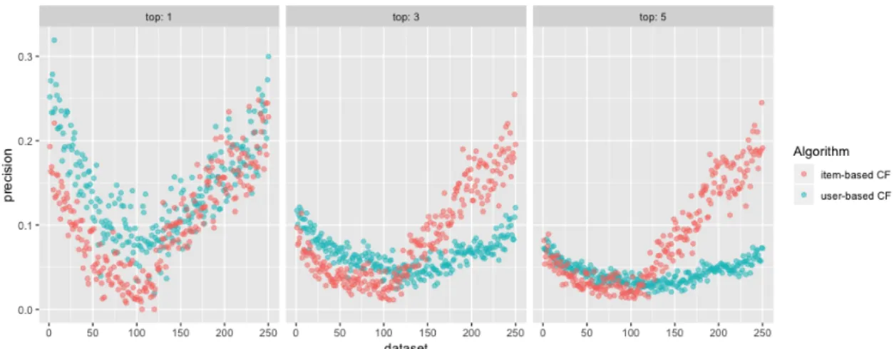
5.1 Results of base-level evaluation on palcoprincipal-playlist dataset. . . 43

5.2 Results of base-level evaluation on amazon-movies dataset. . . 43

5.3 Results of base-level evaluation on movielens1m and palcoprincipal-playlist datasets. 45 5.4 Intra-domain performance evaluation scheme. . . 45

5.5 Inter-domain performance evaluation scheme. . . 47

5.6 Source (Ds) and target (Dt) datasets selection: meta-models created with random samples (without trajectories). . . 48

5.7 Results of meta-level evaluation on palcoprincipal-playlist dataset — Mean value of attributes concentration. . . 48

5.8 Results of meta-level evaluation on palcoprincipal-playlist dataset — Mean of column count. . . 49

5.9 Results of meta-level evaluation on palcoprincipal-playlist dataset — Entropy of row count. . . 49

5.10 Results of meta-level evaluation on palcoprincipal-playlist dataset — Kurtosis of row count. . . 50

5.11 Results of meta-level evaluation on palcoprincipal-playlist dataset — Max value of row count. . . 50

5.12 Results of meta-level evaluation on palcoprincipal-playlist dataset — Number of zeros on entire dataset. . . 51

5.13 Results of meta-level evaluation on palcoprincipal-playlist dataset — Number of binary attributes. . . 51

5.14 Results of meta-level evaluation on palcoprincipal-playlist dataset — Mean value of attributes entropy. . . 52

(16)

LIST OF FIGURES

5.15 Results of meta-level evaluation on palcoprincipal-playlist dataset — Entropy of column count. . . 52

5.16 Results of meta-level evaluation on palcoprincipal-playlist dataset — Kurtosis of column count. . . 53

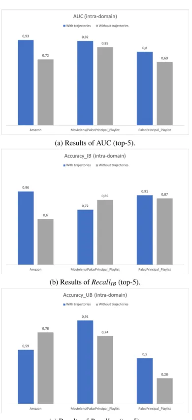
5.17 Comparison between RF meta-models created with trajectories and random sam-ples (intra-domain test). . . 60

5.18 Comparison between RF meta-models created with trajectories and random sam-ples — amazon-movies (inter-domain test). . . 61

5.19 Comparison between RF meta-models created with trajectories and random sam-ples — movielens1m/palcoprincipal-playlist (inter-domain test). . . 62

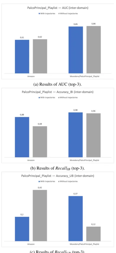
5.20 Comparison between RF meta-models created with trajectories and random sam-ples — palcoprincipal-playlist (inter-domain test). . . 63

5.21 Variable importance of RF meta-models. . . 65

A.1 Results of base-level evaluation on palcoprincipal-playlist dataset (recall metric). 78

A.11 Results of base-level evaluation on palcoprincipal-playlist dataset (column-wise transformations). . . 81

B.1 Results of meta-level evaluation on palcoprincipal-playlist dataset — Gini of col-umn count. . . 86

B.2 Results of meta-level evaluation on palcoprincipal-playlist dataset — Entropy of column mean. . . 86

(17)

LIST OF FIGURES

B.3 Results of meta-level evaluation on palcoprincipal-playlist dataset — Sparsity of entire dataset. . . 87

B.4 Results of meta-level evaluation on palcoprincipal-playlist dataset — Mean value of attributes concentration. . . 87

B.5 Results of meta-level evaluation on palcoprincipal-playlist dataset — Mean of column count. . . 88

B.6 Results of meta-level evaluation on palcoprincipal-playlist dataset — Entropy of row count. . . 88

B.7 Results of meta-level evaluation on palcoprincipal-playlist dataset — Kurtosis of row count. . . 89

B.8 Results of meta-level evaluation on palcoprincipal-playlist dataset — Max value of row count. . . 89

B.9 Results of meta-level evaluation on palcoprincipal-playlist dataset — Number of binary attributes. . . 90

B.10 Results of meta-level evaluation on palcoprincipal-playlist dataset — Number of zeros on entire dataset. . . 90

B.11 Results of meta-level evaluation on palcoprincipal-playlist dataset — Mean value of attributes entropy. . . 91

B.12 Results of meta-level evaluation on palcoprincipal-playlist dataset — Entropy of column count. . . 91

B.13 Results of meta-level evaluation on palcoprincipal-playlist dataset — Kurtosis of column count. . . 92

(18)

(19)

List of Tables

2.1 Sample rating matrix (on a 5-star scale). . . 10

2.2 Confusion matrix. . . 15

4.1 Datasets used in the base-level experiments. . . 33

4.2 List of metafeatures considered in this study. . . 39

5.1 Summary of meta-level results. . . 44

5.2 Results of meta-models performance (training set). . . 47

5.3 Results of meta-models performance (test set). . . 53

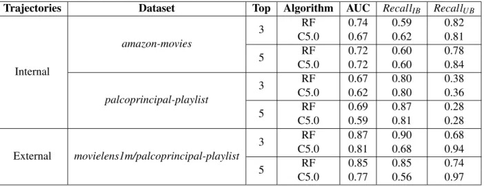
5.4 Results of testing amazon-movies meta-model on remaining selected datasets. . . 55

5.5 Results of testing movielens1m/palcoprincipal-playlist meta-model on remaining selected datasets. . . 55

5.6 Results of testing palcoprincipal-playlist meta-model on remaining selected datasets. 55 5.7 Results of testing amazon-movies meta-model on remaining selected datasets, con-sidering the application of undersampling technique. . . 55

5.8 Results of testing movielens1m/palcoprincipal-playlist meta-model on remaining selected datasets, considering the application of undersampling technique. . . 56

5.9 Results of testing palcoprincipal-playlist meta-model on remaining selected datasets, considering the application of undersampling technique. . . 56

5.10 Results of testing meta-models created without trajectories, on test sets containing meta-examples generated through dataset transformations process. . . 58

5.11 Results of testing amazon-movies meta-model, created without trajectories, on (remaining) test sets containing meta-examples generated through dataset trans-formations process. . . 58

5.12 Results of testing movielens1m/palcoprincipal-playlist meta-model, created with-out trajectories, on (remaining) test sets containing meta-examples generated through dataset transformations process. . . 58

5.13 Results of testing palcoprincipal-playlist meta-model, created without trajecto-ries, on (remaining) test sets containing meta-examples generated through dataset transformations process. . . 59

5.14 Summary comparison between performance results obtained from meta-models created with trajectories and random samples (intra and inter-domain tests). . . . 59

B.1 Results of palcoprincipal-playlist meta-model performance (training set) — Re-gression task. . . 86

B.2 Results of palcoprincipal-playlist meta-model performance (test set) — Regres-sion task. . . 87

(20)

(21)

Abbreviations

AUC Area Under the Curve CB Content-based

CF Collaborative Filtering DM Data Mining

GBM Gradient Boosting Machine MAE Mean Absolute Error MF Matrix Factorization ML Machine Learning MtL Metalearning

NFLT No-Free-Lunch Theorem NIR No Information Rate NN Nearest Neighborhood

PCA Principal Component Analysis RF Random Forest

RMSE Root Mean Square Error

ROC Receiver Operating Characteristics RS Recommender System

(22)

(23)

Chapter 1

Introduction

We are daily overwhelmed with choices and options. What to buy? What to wear? What movie to see? What book to read? Furthermore, the sizes of these decision domains are frequently massive. The tremendous growth in the amount of available information has created a potential challenge of information overload [IFO15]. Technology has dramatically reduced the barriers to publishing and distributing information. Beyond that, the amount of information in the world is increasing far more quickly than our ability to process it. Users have to spend more time and energy searching for their desired information. Even simple decisions — what movie should I watch this weekend? — can be difficult without prior direct knowledge of the candidates. This has increased the demand for Recommender Systems more than ever.

Recommender Systems (RSs) are information filtering systems that deal with the problem of information overload. They filter key fragments, out of large amount of dynamically generated information, according to user preferences or observed behavior [KR12]. A RS has the ability to predict whether a particular user would prefer an item or not, based on the user’s profile. They can now be found in many modern applications that expose the user to a huge collection of items. Such systems typically provide the user with a list of recommended items they might prefer, or supply guesses of how much the user might prefer each item. These systems help users to decide on most appropriate items, and ease the task of finding preferred items in the collection.

Historically, people have relied on recommendations and mentions from their peers or the advice of experts to support decisions and discover new material. Nevertheless, these methods of recommending new things have their limits, particularly for information discovery [ERK07]. Computer-based systems provide the opportunity to expand the set of people from whom users can obtain recommendations. They also enable us to mine user’s history and stated preferences for patterns that neither they nor their peers identify, potentially providing a more finely-tuned selection experience.

Nowadays RSs are an accepted technology used by market leaders in several industries (e.g., Facebook recommends new friends, Youtube recommends videos, Netflix recommends movies, Amazonrecommends books). RSs apply statistical and knowledge discovery techniques to the problem of making product recommendations based on previously recorded data. Such

(24)

recom-Introduction

mendations improve the decision making process, by helping the customer to find the products he wants faster. They also promote cross-selling by suggesting additional products and can improve customer loyalty through creating a value-added relationship [Hah11]. Based on purchase and browsing history, they recommend items for the user to consider purchasing. As an example, the movie rental provider Netflix displays predicted ratings for every displayed movie, in order to help the user decide which movie to rent. Also the online book retailer Amazon provides a list of other books that are bought by users who buy a specific book. A significant motivation for doing this is to increase sales volume — customers may purchase an item if it is suggested to them, but might not seek it out otherwise.

Over the last two decades there has been a vast amount of research in the RS field, mostly focusing on designing new algorithms for recommendations [GS09]. This gain in popularity has led to a wide variety of algorithms in such a way that choosing the best one for each problem became a hard task. RS algorithms typically perform differently in various domains. Therefore, it is important from the research perspective, as well as from a practical view, to be able to decide on an algorithm that matches each problem.

1.1 Motivation and Goals

One of the most successful techniques for RS, called Collaborative Filtering (CF), has been de-veloped and improved over the last few years to the point where a wide variety of algorithms exist for generating recommendations. Besides different algorithms may perform better or worse on different datasets, theoretical knowledge about the performance of those algorithms is miss-ing [CSdC16]. Therefore, clearly identifying the best algorithm for a given purpose has proven challenging. Furthermore, in real world RSs, it is reasonable to approach ratings data as a data stream: ratings are continuously being generated, and we have no control over the data rate or the ordering of the arrival of new ratings [VJG14]. A successful RS has to account for changes in data and adapt to them, selecting the best algorithm to use in each case. However, the empiri-cal research that has taken place produced non-generalizable results due to the absence of a large number of datasets [CSdC16]. Nevertheless, the solution does not lie in randomly generated data because it is unlikely that it reflects a real world distribution. In addition, for a given problem, in order to find the best algorithm, the No-Free-Lunch Theorem (NFLT) should remind us that, how well the algorithm will do is determined by how aligned the algorithm is with the actual problem at hand [WM97]. This means that randomly selecting a good algorithm without making any struc-tural assumptions on the problem is similar to the proverbial "needle in the haystack". Thus, we need to consider the problem and its data, and act accordingly, engineering a solution with a good fit to the task at hand. From the scientific perspective it is also important to identify the limitations of existing algorithms. With these limitations in mind, the development of new algorithms, that fix the existing weaknesses, could be promoted.

(25)

Introduction

address this issue, a Metalearning (MtL) approach is proposed. It consists of relating data char-acteristics (metafeatures) to the performance of recommendation algorithms. These metafeatures are expected to contain some useful information about the relative performance of the algorithms. Furthermore, it is intended that the extracted knowledge could be generalizable and, therefore, applied on other datasets. The generalization of a MtL process requires a large and diverse collec-tion of datasets. Thus, the main goal is to develop a methodology that generates new datasets by manipulating existing ones, such that they are useful for understanding algorithm behavior using MtL approaches (including in the case of evolving data, such as in RS). The proposed approach consists of the iterative application of transformations (morphing) on real datasets which repre-sent an interesting behavior of algorithms (e.g., algorithm A is better than B on one dataset but the opposite happens in the other). Determining the turning point of the algorithm performance, and carefully analyzing what happens around the boundary, could be crucial to identify a relationship between algorithm performance and data characteristics. Those transformations could be simple and applied in a random way, (i.e., bit flipping, rows/columns switching) or more complex, like those applied in an ordered way (i.e., switch the most similar row/column first). Then, the goal is to identify patterns between metafeatures variation and algorithm performance. The algorithm selec-tion problem could be formulated as a classificaselec-tion task, where the target attribute is the best CF algorithm, according to each performance metric. Thus, it would be possible to predict the most promising algorithm and explain why RS algorithms perform better or worst. Beyond the practical issue of selecting the most appropriate algorithm for each problem, the relationship between al-gorithm performance and data characteristics represents a very important topic from the scientific perspective — understand the behavior of existing algorithms and identify their limitations.

1.2 Research Questions

In this study, we propose dataset morphing as a process of generating multiple datasets, that will be considered as meta-examples at the meta-level. We believe this process could be useful to enrich the metadata and, therefore, improve the quality of the available metaknowledge.

Thus, this dissertation is based on the following hypothesis:

It is possible to manipulate existing data to improve the results of MtL processes, that learn the relationship between the performance of RS algorithms and data characteristics.

Based on this, two different groups of research questions will be answered. Firstly, related to the identification of metafeatures that contain some useful information about the relative perfor-mance of the algorithms i.e., metafeatures that vary accordingly with algorithm perforperfor-mance:

• RQ1.1 Does morphing lead to a sequence of datasets with clear relationships between their characteristics (i.e., metafeatures) and algorithm performance?

(26)

Introduction

Secondly, related to the meta-models created at the meta-level. These models will enable us to evaluate whether the extracted (meta)knowledge is generalizable not only across samples of the same dataset (Figure1.1), but also across domains (Figure1.2). It will be also possible to validate the importance of dataset transformations resulting from the proposed methodology:

• RQ2.1 Does meta-data obtained from morphing different datasets of the same domain lead to better meta-knowledge?

• RQ2.2 Does meta-data obtained from morphing datasets of different domains lead to better meta-knowledge?

• RQ2.3 Does meta-data obtained from morphing datasets lead to better meta-knowledge when compared to meta-data obtained from random samples?

Figure 1.1: Transfer of (meta)knowledge across samples of the same meta-dataset.

Figure 1.2: Transfer of (meta)knowledge across samples of different meta-datasets.

This dissertation tries to answer the previous research questions with the aim of satisfying the proposed goals (Section1.1).

(27)

Introduction

1.3 Document Structure

The remainder of this document is structured as follows:

• Chapter2, Background, provides a literature review on RSs, focusing on CF and the eval-uation protocol. It also presents a brief review on MtL, regarding data characterization and RS algorithm selection problem;

• Chapter3, Morphing Recommendation Datasets, describes in detail the proposed method-ology to address the problem;

• Chapter4, Empirical Evaluation, presents the experimental setup at base and meta-levels. Some implementation details are also mentioned;

• Chapter5, Experimental Results, contains the results of both evaluation experiments; • Chapter6, Conclusions & Future Work, holds the main conclusions and points out possible

(28)

(29)

Chapter 2

Background

This chapter presents an overview of all subjects covered in this dissertation: Recommender Sys-tems (Section2.1), Metalearning (Section2.2) and Metalearning for Recommender Systems (Sec-tion2.3).

2.1 Recommender Systems

RSs analyze patterns of user interest in items to provide personalized recommendations that suit a user’s preference. Therefore, they have become fundamental applications in electronic commerce and information access in such a way that today RSs are an accepted technology used by mar-ket leaders in several industries (e.g., Facebook recommends new friends, Youtube recommends videos, Netflix recommends movies, Amazon recommends books). This section presents the key aspects of RSs, with a focus on CF. It also describes how the performance of RSs are usually evaluated.

2.1.1 Definition

RSs apply data analysis techniques to the problem of helping users find the items they want, by producing a predicted likeliness score or a list of top-N recommended items for a given user. Item is the general term used to denote what the system recommends to users. A RS normally focuses on a specific type of item (e.g., books or movies) and the core recommendation technique, used to generate the recommendations, is customized to provide useful and effective suggestions for that specific type of item [RSR15]. Item recommendations can be made using different methods. In their simplest form, personalized recommendations are offered as ranked lists of items. In performing this ranking, RSs try to predict what the most suitable products or services are, based on the user’s preferences and constraints. In order to complete such a computational task, RSs collect information from users regarding their preferences, which are either explicitly expressed (e.g., as ratings for items) or are inferred by interpreting the actions of the user. For instance, a

(30)

Background

RS may consider the navigation to a particular product page as an implicit sign of preference for the items shown on that page [RSR15]. In recent years, RSs have proven to be a valuable means of handling the information overload problem. Ultimately a RS addresses this phenomenon by pointing a user toward new, not-yet-experienced items that may be relevant to the user’s current task. Upon a user’s request, which can be articulated depending on the recommendation approach by the user’s context and need, RSs generate recommendations using various types of knowledge and data about users, the available items, and previous transactions stored in databases. The user can then browse the recommendations. One may accept them or not and may provide, immediately or at a later stage, implicit or explicit feedback. This user action and feedback can be stored in the recommender database and may be used for generating new recommendations in the coming user-system interactions [RSR15].

In describing RSs, we typically focus on two tasks: rating prediction and item recommenda-tion. In rating prediction, the goal is to train models to accurately estimate the ratings users would give to items. On the other hand, item recommendation aims to recommend ordered lists of items, according to the preference of the users. In its most common formulation, the recommendation problem is reduced to the problem of estimating ratings for the items that have not been seen by a user. Once we can estimate ratings for the yet unrated items, we can recommend the item(s) with the highest estimated rating(s) to the user.

In order to implement its core function, identifying useful items for the user, a RS must predict that an item is worth recommending. In order to do this, the system must be able to predict the utility of some items, or at least compare the utility of some items, and then decide which items to recommend based on this comparison. More formally, the recommendation problem can be formulated as follows: let U be the set of all users and let I be the set of all possible items that can be recommended, such as books, movies or restaurants. Let f be a utility function that measures the usefulness of item i to user u, i.e., f : U × I → R, where R is a totally ordered set (i.e., non-negative integers or real numbers within a certain range). Then, for each user u ∈ U , we want to choose such i0∈ I that maximizes the user’s utility [AT05]:

∀u ∈ U, i0_u= maxi∈If(u, i) (2.1)

In RSs, the utility of an item is usually represented by a rating, which indicates how a particular user liked a particular item (e.g., user A gave the movie Star Wars the rating of 4 (out of 5)). Nevertheless, the utility f is usually not known on the whole U × I space, but only on some subset of it. In RSs, utility is initially defined only on the items previously rated by the users. This means fneeds to be extrapolated to the whole space U × I. Thus, the fundamental task of RS is to predict the value of f over pairs of users and items, or in other words, to compute ˆf, i.e., the estimation, computed by the RS, of the true function f . Consequently, having computed this prediction for the active user on a set of items, the system will recommend the items with the largest predicted utility. Regarding the definition of the item recommendation task, we introduce the following notation: Iu is the set of items rated or purchased by user u and Ui is the set of users who have

(31)

Background

rated or purchased i. The data structure used in CF is named rating matrix R, with ru,ibeing the

rating user u provided for item i, rubeing the vector of all ratings provided by user u and ribeing

the vector of all ratings provided for item i. ¯ruand ¯riare the average ratings of a user u or an item

i, respectively. The user for whom a recommendation is wanted, is referred to us as the active user ua. ˆru,iexpresses the predicted rating of the user u for an item i, i.e., ˆf(u, i).

Thus, depending on the type of feedback, it is possible to distinguish two recommendation tasks:

• Rating prediction where the feedback is explicit: ru,iare numbers representing ratings of

users for items, and ˆru,i= ˆf(u, i) expresses the predicted rating of the user u for an item i;

• Item recommendation where the feedback is implicit: ru,iare zeros and ones representing

the absence or presence, respectively, of an interaction between users and items, and ˆru,i=

ˆ

f(u, i) expresses the predicted likelihood of a positive implicit feedback (ranking score) of the user u for an item i.

2.1.2 Algorithmic approaches

There are several different types of RSs that vary in terms of the addressed domain and the knowl-edge used, but especially with regard to the recommendation algorithm, i.e., how the prediction of the utility of a recommendation is made. RSs are usually classified into the following cate-gories [RSR15]:

• Content-Based: The system learns to recommend items that are similar to the ones that the user liked in the past. The similarity of items is calculated based on the features associated with the items. For example, if a user has positively rated a movie that belongs to the action genre, then the system can learn to recommend other movies from this genre;

• Collaborative Filtering: The system makes recommendations to the active user based on items that other users with similar tastes liked in the past. The similarity in taste of two users is calculated based on the similarity in the rating history of the users. CF is considered to be the most popular and widely implemented technique in RS.

The details of each category are described below.

2.1.2.1 Content-Based

Content-Based (CB) recommendation techniques aim at matching the attributes of the user profile against the attributes of the items. In most cases, the items’ attributes are simply keywords that are extracted from the items’ descriptions [RSR15]. This approach is based on the idea that if we can elicit the preference structure of a user concerning item attributes then we can recommend items which rank high for the user most desirable attributes. Typically, the preference structure can be elicited by analyzing which items the user prefers. Items that are mostly related to the positively rated items are recommended to the user.

(32)

Background

In this technique, the profile of other users is not needed since they do not influence recom-mendation. Also, if the user profile changes, this technique still has the potential to adjust its recommendations within a very short period of time. However, the major disadvantage of this approach is the need to have an in-depth knowledge and description of the features of the items in the profile. So, the effectiveness of CB depends on the availability of descriptive data. Another se-rious problem of CB technique is content overspecialization [ZI02]. Users are restricted to getting recommendations similar to items already defined in their profiles.

2.1.2.2 Collaborative Filtering

CF is, probably, the most successful recommendation technique to date. The basic idea of CF-based algorithms is to provide item recommendations or predictions CF-based on the opinions of other like-minded users. The opinions of users can be obtained explicitly from the users or by using some implicit measures.

The information domain for a CF system consists of users which have expressed preferences for various items. A preference expressed by a user for an item is called a rating and is frequently represented as a {User, Item, Rating} triple. These ratings can take many forms, depending on the system in question. Some system use real (or integer) valued rating scales such as 0-5 stars, while others use binary (like/dislike) scales. Binary ratings, such as "has purchased", are particularly common in e-commerce deployments. The set of all rating triples forms a sparse matrix referred to as the rating matrix, R. {User, Item} pairs where the user has not rated the item are unknown values in this matrix. Table 2.1shows a rating matrix example for three users and four movies. Cells marked ’?’ represent unknown values (the user has not rated that movie).

Table 2.1: Sample rating matrix (on a 5-star scale).

Titanic The Godfather Star Wars Forrest Gump

User A ? 4 4 5

User B 4 ? 2 ?

User C 5 5 3 ?

CF approaches can be grouped in the two general classes of memory-based and model-based methods [BOHG13]. In memory-based (or neighborhood-based) approaches the user-item ratings stored in the system are directly used to predict ratings for new items. This can be done in two ways known as user-based or item-based recommendation. User-based systems evaluate the interest of the active user for an item, using the ratings for this item by other users, called neighbors, that have similar rating patterns. The neighbors of the target user are typically the users whose ratings are most correlated to the target user’s ratings. The assumption is that users with similar preferences will rate items similarly. Thus missing ratings for a user can be predicted by first finding a neighborhood of similar users and then aggregate the ratings of these users to form a prediction. The neighborhood for the active user, N(ua) ⊂ U , is defined in terms of similarity

(33)

Background

all users within a given similarity threshold. Popular similarity measures for CF are the Pearson correlation coefficientand the Cosine similarity. These similarity measures are defined below in Section 2.1.2.3. Once the users in the neighborhood are found, their ratings are aggregated to form the predicted rating for the active user. The easiest form is to just average the ratings in the neighborhood [Hah11]: ˆra j= 1 N(ua)_(i)∈N(u

∑

a) ri, j, (2.2)

In order to create a top-N recommendation list, the items must be ordered by predicted rating. User-based methods usually provide more original recommendations, which may lead users to a more satisfying experience [RSR15].

On the other hand, item-based approaches predict the rating of a user for an item based on the ratings of the user for similar items. In such approaches, two items are similar if several users of the system have rated these items in a similar fashion. The assumption behind this approach is that users will prefer items that are similar to other items they like. A similarity matrix containing all item-to-item similarities is calculated, using a given measure. Popular similarity measures are Pearson correlation and Cosine similarity. All pairwise similarities are stored in a similarity matrix. To make a recommendation, similarities are used to calculate a weighted sum of the user’s ratings for related items. This idea can be formalized as follows. Denote by Nu(i) the items rated

by user u most similar to item i. The predicted rating of u for i is obtained as a weighted average of the ratings given by u to the items of Nu(i) [RSR15]:

ˆru,i=

∑j∈Nu(i)wi jru j

∑j∈Nu(i)|wi j|

(2.3)

where wi jrepresents the similarity between items i and j.

In contrast to memory-based systems, which use the stored ratings directly in the prediction, model-based approaches use these ratings to learn a predictive model. Salient characteristics of users and items are captured by a set of model parameters, which are learned from training data and later used to predict new ratings [NDK15]. There are various model-based CF algorithms including Bayesian Networks, Clustering Models, and Latent Semantic Models such as Singu-lar Value Decomposition (SVD), Principal Component Analysis (PCA) and Probabilistic Matrix Factorization for dimensionality reduction of rating matrix.

2.1.2.3 Similarity measures

There are some different ways to compute similarity. Here we present two such approaches: correlation-based and cosine-based. In the correlation-based approach, the Pearson correlation coefficient is used to measure similarity. This approach computes the statistical correlation

(34)

(Pear-Background

son’s r) between two users common ratings to determine their similarity. The correlation is com-puted as follows:

sim(u, v) = ∑i∈Iu∩Iv(ru,i− ¯ru)(rv,i− ¯rv)

q

∑i∈Iu∩Iv(ru,i− ¯ru)

2q

∑i∈Iu∩Iv(rv,i− ¯rv)

2

, (2.4)

where Iu∩ Ivrepresents the set of all items co-rated by both users u and v. Pearson correlation

suf-fers from computing similarity between users with few ratings in common. This can be mitigated by setting a threshold on the number of co-rated items necessary for full agreement (correlation of 1) and scaling the similarity when the number of co-rated items falls below this threshold [ERK07].

Cosine similarity is different from Pearson correlation since it is a vector-space model. It is based on linear algebra rather than statistical approach. It measures the similarity between two |I|-dimensional vectors based on the angle between them. The similarity between two users u and vcan be defined as follows:

sim(u, v) = cos(~u,~v) = ~u ·~v ||~u||₂× ||~v||₂ = ∑iru,irv,i q ∑ir2u,i q ∑ir2v,i , (2.5)

where ~u and ~v represent the row vectors in R, ~u ·~v denotes the dot-product between the vectors ~u and ~v and the || · ||2 the l2-norm of a vector. Cosine similarity between item rating vectors is

the most popular similarity metric, as it is simple, fast and produces good predictive accuracy [ERK07]. It is widely used in text mining to compare documents, represented as word vectors.

Nevertheless, some other similarity measures have been proposed regarding binary data. This was motivated by the fact that, in binary data, missing ratings (zeros) could mean that either the user does not like the item or does not know about it. On the other hand, from ones we could infer that the user has a preference for an item. Thus, two strategies are possible: assume all missing ratings are negative examples or assume that all missing ratings are unknown. If we assume that users typically favor only a small fraction of the items, and thus most items with no rating will be indeed negative examples, then we have no missing values and can use the approaches described above. However, if we consider all zeros as missing values, then this leads to the problem that we cannot compute similarities using Pearson correlation or Cosine similarity since the no missing parts of the vectors only contain ones. A similarity measure which only focuses on matching ones, preventing the problem with zeros, is the Jaccard index [Hah11]:

simJaccard(X ,Y ) =

X∩Y

X∪Y, (2.6)

where X and Y are the sets of the items with a 1 in user profiles ua and ub, respectively. The

Jaccard index can be used between users for user-based CF or between items for item-based CF as described above.

(35)

Background

2.1.2.4 Content-Based vs Collaborative Filtering

The general principle of CB methods is to identify the common characteristics of items that have received a favorable rating from a user, and then recommend to this user new items that share these characteristics. RSs based purely on content generally suffer from the problems of limited content analysis and overspecialization. Limited content analysis occurs when the system has a limited amount of information on its users or the content of its items. For instance, privacy issues might refrain a user from providing personal information, or the precise content of items may be difficult or costly to obtain for some types of items, such as music or images. Another problem is that the content of an item is often insufficient to determine its quality. Over-specialization, on the other hand, is a side effect of the way in which CB systems recommend new items, where the predicted rating of a user for an item is high if this item is similar to the ones liked by this user. For example, in a movie recommendation application, the system may recommend to a user a movie of the same genre or having the same actors as movies already seen by this user. Because of this, the system may fail to recommend items that are different but still interesting to the user [NDK15].

Instead of depending on content information, CF approaches use the rating information of other users and items in the system. The key idea is that the rating of a target user for a new item is likely to be similar to that of another user, if both users have rated other items in a similar way. Likewise, the active user is likely to rate two items in a similar fashion, if other users have given similar ratings to these two items [NDK15].

CF approaches overcome some of the limitations of CB ones. For instance, items for which the content is not available or difficult to obtain can still be recommended to users through the feedback of other users. Furthermore, CF recommendations are based on the quality of items as evaluated by peers, instead of relying on content that may be a bad indicator of quality. Finally, unlike CB systems, CF ones can recommend items with very different content, as long as other users have already shown interest for these different items. Despite the success of CF approach, it is possible to identify some potential issues like cold-start [BOHG13] and data sparsity [Bur02] problems. The first one refers to a situation where a RS does not have sufficient information about a user or item, in order to make relevant predictions. The second one occurs due to the absence of information, that is, when only a few of the total number of items available in a database are rated by users. Sparse user-item matrix means inability to successfully locate neighbors and it results in weak recommendations.

2.1.3 Evaluation

Evaluation of RSs is definitely an important topic. Evaluation is required at different stages of the system’s life cycle and for various purposes. At design time, evaluation is required to verify the selection of the appropriate recommender approach. In the design phase, evaluation should be im-plemented off-line and the recommendation algorithms, i.e., their computed recommendations, are compared with the stored user interactions. An off-line evaluation consists of running several al-gorithms on the same datasets of user interactions (e.g., ratings) and comparing their performance.

(36)

Background

Off-line experiments can measure the quality of the chosen algorithm in fulfilling its recommen-dation task [RSR15]. They are performed by using a pre-collected dataset of users choosing or rating items. Using this dataset we can try to simulate the behavior of users that interact with a RS. In doing so, we assume that the user behavior when the data was collected will be similar enough to the user behavior when the RS is deployed, so that we can make reliable decisions based on the simulation. Offline experiments are attractive because they require no interaction with real users, and thus allow us to compare a wide range of candidate algorithms at a low cost [SG11].

Typically, given a rating matrix R, recommender algorithms are evaluated by first partitioning the users in R into two sets U = Utrain∪ Utest. The rows of R corresponding to the training users

Utrain are used to learn the recommender model. Then, each user ua∈ Utest is seen as an active

user. The training dataset is used to learn the parameters or configure the algorithms used in the analysis step, while the testing dataset is used to estimate performance. To determine how to split U into Utrainand Utest it is possible to use several approaches [Koh95,BG04,BOHB12]:

• Hold-out: randomly assign a predefined proportion of users to the training set and all others to the test set;

• Bootstrap sampling: users are not removed from the population once they have been se-lected, allowing for the same sample to be selected more than once. The users not in the training set form the test set. This procedure has the advantage that, for smaller datasets, it is possible to create larger training sets and still have users left for testing;

• k-fold cross-validation: split U into k sets (called folds) of approximately the same size. Then we evaluate k times, always using one fold for testing and all other folds for learning. The k results can be averaged. This approach makes sure that each user is at least once in the test set, and the averaging produces more robust results and error estimates.

In order to evaluate algorithms off-line, it is necessary to simulate the online process where the system makes predictions or recommendations, and the user corrects the predictions or uses the recommendations. This is usually done by recording historical user data, and then hiding some of these interactions in order to simulate the knowledge of how a user will rate an item, or which recommendations a user will act upon [SG11]. Then, it is measured either how well the predicted rating matches the withheld value or, for the top-N recommendations, if the items in the recom-mended list are rated highly by the user. It is assumed that if a recommender algorithm performed better in predicting the withheld items, it will also perform better in finding good recommendations for unknown items. There are a number of ways to choose the ratings/selected items to be hidden. A common protocol is to use a fixed number of known items or a fixed number of hidden items per test user (so called “Given-x” or “All-but-x” protocols) [SG11]. For the Given-x protocols, for each user x, randomly chosen items are given to the recommender algorithm and the remaining items are withheld for evaluation. For All-but-x, the algorithm gets all but x withheld items.

(37)

Background

The items in the predicted top-N lists and the withheld items liked by the user, for all test users Utest, can be aggregated into a so called confusion matrix, depicted in Table2.2. The confusion

ma-trix shows how many items recommended in the top-N lists (column predicted positive: T P + FP) were withheld items, and thus correct recommendations (TP), and how many where potentially incorrect (FP). The matrix also shows how many items not recommended (column predicted neg-ative: FN + T N) should have actually been recommended, since they represent withheld items (FN). From the confusion matrix, several performance measures can be extracted. The true posi-tive rate (TPR) or Recall measure returns the percentage of true posiposi-tive objects that are classified as positive by the induced classifier. It reaches its highest value when all objects from the positive class are assigned to the positive class by the induced classifier. Recall is also known as Sensitiv-ity. The complement of the Recall is the false negative rate (FNR). The equivalent to the Recall measure for the negative class is the true negative rate (TNR) or Specificity. This measure returns the percentage of objects from the negative class that are classified by the induced classifier as negative. Thus, its value is higher when all negative examples are correctly predicted as negative by the induced classifier. The complement of the Specificity is the false positive rate (FPR). Other measures to evaluate the predictive performance of induced classifiers are the positive predictive value (PPV), also known as Precision, and the negative predictive value.

Table 2.2: Confusion matrix.

actual/predicted positive negative positive True positive (TP) False negative (FN) negative False positive (FP) True negative (TN)

2.1.3.1 Evaluation metrics

For the data mining (DM) task of a RS, the performance of an algorithm depends on its ability to learn relevant patterns in the dataset. The quality of a recommendation algorithm can be evaluated using different measures. A commonly used measure is Accuracy. It is the fraction of correct recommendations out of total possible recommendations. Metrics for measuring the accuracy of recommendation filtering systems are divided into statistical and decision support accuracy metrics [SKKR01]. The suitability of each metric depends on the features of the dataset and the type of tasks that the RS will do.

Statistical accuracy metricsevaluate the accuracy of a filtering technique by comparing pre-dicted ratings directly with the actual user rating. Mean Absolute Error (MAE) and Root Mean Square Error(RMSE) are usually used as statistical accuracy metrics. MAE is the most popular and commonly used. It is a measure of deviation from the true value. Formally,

MAE= 1

(38)

Background

where N is the set of all user-item pairings (i, j), for which we have a predicted rating ˆru,iand

a known rating ru,i. For each ratings-prediction pair < ru,i, ˆru,i> this metric denotes the absolute

error between them. The lower the MAE, the more accurately the recommendation engine predicts user ratings. RMSE penalizes larger errors stronger than MAE. Thus, it is suitable for situations where small prediction errors are not very important. The lower the RMSE is, the better the recommendation accuracy. Formally,

RMSE= s

∑(u,i)∈N(ru,i− ˆru,i)2

N (2.8)

On the other hand, decision support accuracy metrics evaluate how effective a prediction engine is at helping a user select high-quality items from the set of all items. They view prediction process as a binary operation which distinguishes good items from those items that are not good. With this observation, whether a item has a prediction score of 1.5 or 2.5, on a five-point scale, is irrelevant if the user only chooses to consider predictions of 4 or higher. The most commonly used decision support accuracy metrics are precision, recall, F1 and Receiver Operating Characteristics (ROC) [HKTR04]. Precision is the fraction of recommended items that is actually relevant to the user. Formally,

Precision=Correctly recommended items Total recommended items =

T P

FP+ T P (2.9) Recallcan be defined as the fraction of relevant items that are also part of the set of recommended items. Formally,

Recall= Correctly recommended items Total useful recommended items =

T P

FN+ T P (2.10) Typically we can expect a trade off between these quantities — while allowing longer recommen-dation lists typically improves recall, it is also likely to reduce the precision [SG11]. To find an optimal trade-off between them, a single-valued measure like F1 can be used. Formally,

F1 =2 × Precision × Recall Precision+ Recall =

2

1/Precision + 1/Recall (2.11) In applications where the number of recommendations that are presented to the user is not preordained, it is preferable to evaluate algorithms over a range of recommendation list lengths, rather than using a fixed length. Thus, we can compute curves comparing precision to recall, or true positive rate to false positive rate. Curves of the former type are known simply as precision-recall curves, while those of the latter type are known as a receiver operating characteristic curve or ROC curve. While both curves measure the proportion of preferred items that are actually recommended, precision-recall curves emphasize the proportion of recommended items that are preferred while ROC curves emphasize the proportion of items that are not preferred that end up being recommended. We should select whether to use precision-recall or ROC based on the properties of the domain and the goal of the application [SG11]. A possible way to compare the

(39)

Background

efficiency of two systems is by comparing the size of the area under the ROC-curve (AUC), where a bigger area indicates better performance. Figure 2.1 illustrates an example of a ROC graph. To calculate the AUC, this figure shows that the area under the curve can be divided into some trapezoids. Thus the area can be defined by simply adding the areas of the trapezoids.

Figure 2.1: Area Under the ROC-curve (AUC).

2.2 Metalearning

Current DM and machine learning (ML) tools are characterized by a plethora of algorithms but a lack of guidelines to select the right method according to the nature of the problem under anal-ysis [BCSV08]. Since real-world applications are generally time-sensitive, practitioners and re-searchers tend to use only a few available algorithms for data analysis, hoping that the set of assumptions embedded in these algorithms will match the characteristics of the data. Such prac-tice in DM and the application of ML has spurred the research community to investigate whether learning from data is made of a single operational layer – search for a good model that fits the data – or whether there are in fact several operational layers that can be exploited to produce an increase in performance over time [BCSV08]. The latter alternative implies that it should be possible to learn about the learning process itself, and in particular that a system could learn to profit from previous experience to generate additional knowledge that can simplify the automatic selection of efficient models summarizing the data. The aim is to aid users in the task of selecting a suitable predictive model while taking into account the domain of application. End users often lack not

(40)

Background

only the expertise necessary to select a suitable algorithm, but also the availability of many algo-rithms to proceed on a trial-and-error basis. A solution to this problem is attainable through the construction of MtL systems that provide automatic and systematic user guidance by mapping a particular task to a suitable model [BCSV08].

2.2.1 Definition

For the ML community, the idea of measuring statistical features of data to predict classifier per-formance, using ML methods to learn the model, developed into the well-studied field of MtL. MtL is the study of principled methods that exploit metaknowledge to obtain efficient models and solutions by adapting ML and DM processes [BCSV08]. The field of MtL studies how learning systems can become more effective through experience. The main idea is learning about learning algorithm performance. The knowledge gained through experience can be useful in many different settings.

Although, commonly, only a limited number of existing methods are available for use in a given application, the number of these methods may still be too large to rule out extensive ex-perimentation. As there are many alternative algorithms for a given task, the approach of trying out all alternatives and choosing the best one becomes infeasible. An approach followed by many users is to make some preselection of a small number of alternatives based on knowledge about the data and the available methods. The methods are applied to the dataset and the best one is normally chosen taking into account the results. Although feasible, this approach may still require considerable computing time. Additionally, it requires that a highly skilled expert preselect the alternatives, and even the most skilled expert may sometimes fail, and so the best option may be left out [BCSV08]. A MtL approach aims to reduce the number of alternatives to be experimented with.

From the point of view of the user, the goal of a MtL approach for algorithm recommenda-tion can be stated as: save time by reducing the number of alternative algorithms tried out on a given problem with minimal loss in the quality of the results obtained when compared to the best possible ones [BCSV08]. To achieve this goal it is not as important for an algorithm recom-mendation method to accurately predict the true performance of the algorithms as it is to predict their relative performance. Therefore, the task of algorithm recommendation can be defined as the ranking of algorithms according to their predicted performance. To address this problem using a ML approach it is necessary to use data describing the performance of algorithms and the charac-teristics of problems, which we will refer to as metadata. Performance data are used to compute the rankings of the algorithms. These rankings, referred to as target rankings, are the target feature of this learning task. The measures that are used to characterize the problems represent features independent of the particular task and here they are referred to as metafeatures. Based on these concepts, MtL for algorithm recommendation can be defined as: MtL is the use of a ML approach to generate metaknowledge mapping the characteristics of problems (metafeatures) to the relative performance of algorithms. Actually, in order to address the algorithm selection problem, a MtL process induces a metamodel. It can be seen as the metaknowledge able to explain why some

(41)

Background

algorithms perform better than others, in datasets with specific characteristics [CSdC18b]. A sys-tem for algorithm recommendation can be defined as a tool that supports the user in the algorithm selection step of the DM process. Given a dataset, it indicates which algorithm should be used to achieve the best possible results. If sufficient computational resources are available to try several algorithms, it should also indicate which ones should be executed and in which order [BCSV08].

An important topic is the distinction between the traditional view of learning – also known as base-learning – and the one taken by MtL. MtL differs from base-learning in the scope of the level of adaptation. Whereas learning at the base level is focused on accumulating experience on a specific learning task, learning at the meta level is concerned with accumulating experience on the performance of multiple applications of a learning system [BCSV08].

2.2.2 Metafeatures

MtL is based on a database containing information about the performance of a set of algorithms on a set of datasets and about the characteristics of those datasets. The characterization of datasets is probably the issue that has attracted the most attention in MtL research, due to its impor-tance in the process: success is possible only if the metafeatures contain information that is useful for discriminating between the performance of the base-algorithms [BCSV08]. The idea is to gather descriptors about the data distribution that correlate well with the performance of learned models [BCSV08]. The MtL literature usually splits the metafeatures into three main groups [CSdC18b]:

• Statistical and/or information-theoretical: use a set of measures from statistics and in-formation theory to describe the dataset characteristics. This type of metafeatures contains information about properties of datasets, such as size, type, distribution, noise, missing val-ues and redundancy, that usually affect the performance of learning algorithms. Examples of these metafeatures are the number of examples and features in the dataset, entropy, skew-ness and kurtosis of features;

• Model-based: properties extracted from models induced from the dataset (e.g., number of leaf nodes in a decision tree). The assumption is that there is a relationship between algorithm performance and model characteristics which cannot be directly obtained from the data;

• Landmarkers: fast estimates of the algorithm performance on the dataset. They can be either obtained by applying fast and simple algorithms on complete datasets, or by using complete models for samples of datasets (e.g., applying the full decision tree on a sample). Like model-based metafeatures, landmarkers characterize the dataset indirectly. Neverthe-less they go one step further, estimating the performance of one or more algorithms on the task at hand, rather than representing properties of the model. If the performance of the landmarkers is, in fact, related to the performance of the base-algorithms, we can expect this approach to be more successful than the previous ones [BCSV08].

(42)

Background

2.2.3 Algorithmic approaches

A MtL approach for algorithm recommendation involves addressing several issues not only at the meta-level but also at the base-level. At the meta-level, it is necessary, first of all, to choose the type of the target feature, or metatarget, that is, the form of the recommendation that is provided to the user. In some cases, the user may simply be interested in knowing which algorithm is the best. In other cases, more detailed information about the performance of the set of base algorithms may be required. Four different types of metatargets are mostly considered: best algorithm in a set, subset of algorithms, ranking of algorithms and estimated performance of algorithms [BCSV08]. The first type consists of recommending the algorithm that is expected to obtain the best performance in the set of base-algorithms. The second form of recommendation suggests a subset of algorithms that are expected to perform well on the given problem. However, this form of recommendation suggests the algorithms in an unordered way. The lack of order in the subset approach can be remedied if a ranking of the algorithms is provided. Typically, the order indicated in the ranking is the order that should be followed in the experimentation process [BCSV08]. Lastly, if the goal is the actual performance rather than simply relative performance, as offered by the ranking approach, the MtL system should provide recommendations in the form of a value, indicating the performance that each algorithm is expected to achieve [BCSV08].

The type of metatarget determines the type of meta-algorithm, that is, the MtL methods that can be used [BCSV08]. This section discusses meta-algorithms used in existing MtL approaches to the algorithm recommendation problem.

Given their wide availability, many different classification algorithms have been tried for meta-level learning. An extreme example is to use at the meta-meta-level the same set of algorithms that is considered at the base-level [BGc00,PBGC00]. The ten classification algorithms used in these studies are quite diverse, including decision trees, a linear discriminant and neural networks. Such algorithms were compared on several MtL problems and the comparison showed that decision tree and rule-based models obtain the best MtL results [BCSV08].

Not many algorithm recommendation studies carried out so far have used regression rather than classification algorithms at the meta-level. The set of regression algorithms considered is smaller and less diverse. In one earlier work, linear regression, regression trees and model trees were analyzed on the problem of estimating the error of a large number of algorithms. The results indicated that the methods obtain similar performance [BCSV08]. These approaches generate as many metamodels as there are algorithms. It is, thus, not trivial to understand when an algorithm performs better than another one and vice versa [BCSV08].

In MtL, the most commonly used algorithm for learning rankings is based on k-NN [BCSV08]. The choice is essentially motivated by the simplicity of adapting this algorithm for learning rank-ings. In the k-NN approach, it is necessary to predict the ranking of algorithms for a given problem based on the rankings of its k neighbors. Based on the clustering trees algorithm, a general rank-ing method that was proposed, in the context of MtL, is the rankrank-ing trees algorithm [TBD02]. The adaptation for ranking is obtained by replacing the target values (e.g., the accuracy of the

(43)

Background

algorithms) by the corresponding positions in the ranking [BCSV08].

2.3 Metalearning for Recommender Systems

MtL has been used for algorithm selection in RSs [CSdC18a,CSdC18b,CSdC16,GSZ17,ROV13]. These authors manually define metafeatures, which aggregate information from datasets into sin-gle number statistics. For example, the number of instances in the dataset is a simple metafea-ture, the mean or kurtosis of a column is a statistical metafeature. They then use supervised ML to learn the relationships between the metafeatures and the performance of recommenda-tion algorithms on datasets, measured by standard metrics. Although the use of MtL for the selection of CF algorithms has already been investigated, the approaches proposed have limited scope: the set of datasets, recommendation algorithms and metafeatures studied was rather re-stricted [CSdC18a]. An extensive overview of their positive and negative aspects can be seen in a recent survey [CSdC18b]. The literature review shows that most work is performed on CF, with a reduced number of datasets, algorithms and evaluation measures on the base-level. The base-level algorithms are mostly based on NN [CSdC16]. In terms of meta-level, there are several approaches which look at the algorithm selection problem in different and valid approaches. Most work used regression approaches with a wide range of metafeatures. The metafeatures used are of several types [CSdC16]:

• Rating distribution analysis: the number of ratings per user, the average rating per user, the standard rating deviation per user, the ratings entropy, the ratings Gini index and ratings sparsity;

• Neighborhood analysis: the number of neighbors, the average similarity to the top closest 30 neighbors, the clustering coefficient of a group of users, the average Jaccard coefficient per user, group size, social contact level and dissimilarity level;

• General user analysis: the user influence, experience level and activity level;

• General item analysis: the item popularity, the item preference, the user influence and the average item entropy.

More recent work in CF algorithm selection has extended the contributions to the area, in particular with regards to the metafeatures considered, which systematize the data characteristics used in earlier works [CSdC16]. A systematic approach for metafeatures extraction has been proposed recently [CSdC18a].

(44)