Role based behavior analysis

UNIVERSIDADE DE LISBOA FACULDADE DE CIÊNCIAS DEPARTAMENTO DE INFORMÁTICA

ROLE BASED BEHAVIOR ANALYSIS

Ricardo Gonçalves Ramalho

MESTRADO EM SEGURANÇA INFORMÁTICA Novembro 2009

UNIVERSIDADE DE LISBOA FACULDADE DE CIÊNCIAS DEPARTAMENTO DE INFORMÁTICA

ROLE BASED BEHAVIOR ANALYSIS

Ricardo Gonçalves Ramalho

Orientador Hyong S. Kim Co-Orientador

Paulo Sousa

MESTRADO EM SEGURANÇA INFORMÁTICA Novembro 2009

I

Resumo

Nos nossos dias, o sucesso de uma empresa depende da sua agilidade e capacidade de se adaptar a condições que se alteram rapidamente. Dois requisitos para esse sucesso são trabalhadores proactivos e uma infra-estrutura ágil de Tecnologias de Informação/Sistemas de Informação (TI/SI) que os consiga suportar. No entanto, isto nem sempre sucede. Os requisitos dos utilizadores ao nível da rede podem não ser completamente conhecidos, o que causa atrasos nas mudanças de local e reorganizações. Além disso, se não houver um conhecimento preciso dos requisitos, a infra-estrutura de TI/SI poderá ser utilizada de forma ineficiente, com excessos em algumas áreas e deficiências noutras. Finalmente, incentivar a proactividade não implica acesso completo e sem restrições, uma vez que pode deixar os sistemas vulneráveis a ameaças externas e internas. O objectivo do trabalho descrito nesta tese é desenvolver um sistema que consiga caracterizar o comportamento dos utilizadores do ponto de vista da rede.

Propomos uma arquitectura de sistema modular para extrair informação de fluxos de rede etiquetados. O processo é iniciado com a criação de perfis de utilizador a partir da sua informação de fluxos de rede. Depois, perfis com características semelhantes são agrupados automaticamente, originando perfis de grupo. Finalmente, os perfis individuais são comprados com os perfis de grupo, e os que diferem significativamente são marcados como anomalias para análise detalhada posterior. Considerando esta arquitectura, propomos um modelo para descrever o comportamento de rede dos utilizadores e dos grupos. Propomos ainda métodos de visualização que permitem inspeccionar rapidamente toda a informação contida no modelo.

O sistema e modelo foram avaliados utilizando um conjunto de dados reais obtidos de um operador de telecomunicações. Os resultados confirmam que os grupos projectam com precisão comportamento semelhante. Além disso, as anomalias foram as esperadas, considerando a população subjacente. Com a informação que este sistema consegue extrair dos dados em bruto, as necessidades de rede dos utilizadores podem sem supridas mais eficazmente, os utilizadores suspeitos são assinalados para posterior análise, conferindo uma vantagem competitiva a qualquer empresa que use este sistema.

Palavras-chave: análise de comportamento de rede, análise do perfil de utilizadores, comportamento de utilizador, fluxos de rede, fluxos aplicacionais, prospecção de dados, detecção de anomalias.

II

Abstract

In our days, the success of a corporation hinges on its agility and ability to adapt to fast changing conditions. Proactive workers and an agile IT/IS infrastructure that can support them is a requirement for this success. Unfortunately, this is not always the case. The user’s network requirements may not be fully understood, which slows down relocation and reorganization. Also, if there is no grasp on the real requirements, the IT/IS infrastructure may not be efficiently used, with waste in some areas and deficiencies in others. Finally, enabling proactivity does not mean full unrestricted access, since this may leave the systems vulnerable to outsider and insider threats. The purpose of the work described on this thesis is to develop a system that can characterize user network behavior.

We propose a modular system architecture to extract information from tagged network flows. The system process begins by creating user profiles from their network flows’ information. Then, similar profiles are automatically grouped into clusters, creating role profiles. Finally, the individual profiles are compared against the roles, and the ones that differ significantly are flagged as anomalies for further inspection. Considering this architecture, we propose a model to describe user and role network behavior. We also propose visualization methods to quickly inspect all the information contained in the model.

The system and model were evaluated using a real dataset from a large telecommunications operator. The results confirm that the roles accurately map similar behavior. The anomaly results were also expected, considering the underlying population. With the knowledge that the system can extract from the raw data, the users network needs can be better fulfilled, the anomalous users flagged for inspection, giving an edge in agility for any company that uses it.

Keywords: network behavior analysis, user profiling, user behavior, network flow, application flow, data mining, anomaly detection.

III

Acknowledgments

I would like to thank Professor Hyong Kim for his guidance and advice. His experience was vital to guide this project to a successful and timely conclusion. I would also like to thank Professor Paulo Sousa for his dedication in helping making this thesis an enjoyable reading experience.

To my colleagues from MSIT-IS class of 2008/2009, for all the companionship, debates and support throughout the course. To the colleagues from last year’s course for their helpful tips and advice. To John Payne for all the brainstorming sessions, lengthy discussions and advice. A special thanks to the group that travelled far and wide with me to make their thesis a unique experience.

To José Alegria for his support, incentive and trust in my abilities. To Tiago Carvalho and Luís Costa, for making the corporate – academic interface possible.

To my family and friends, who still remember me after these long 16 months!

Most of all, a very special thanks to my dearest Cláudia, for all her support, patience and dedication. This is just the remainder…

IV

Contents

2.3.3. Predictive modeling (classification) ...15

2.3.4. Anomaly detection ...15 2.3.5. Association analysis...17 2.4. Related work...17 2.4.1. Traffic classification...17 2.4.2. Data mining ...20 2.4.3. User behavior ...21

3 Model and architecture ...23

3.1. Architecture...23

3.2. Profiler ...23

3.3. User profile model...24

3.4. Roler ...27 3.5. Roles model ...28 3.6. Anomaly detector...31 3.7. Temporal analysis ...31 3.8. Previous models ...31 3.8.1. PCA / SVD ...32

V

3.8.2. Overly simplistic model ...32

3.8.3. Fixed categories on individual attributes (traffic/flows/duration) ...33

3.8.4. Variable categories on all attributes ...33

4 Results...35 4.1. Single analysis...35 4.1.1. Role visualization...39 4.1.2. Anomaly detector...42 5 Deployment...45 5.1. System components ...45 5.1.1. Probes...45 5.1.2. Event repository (DB) ...45 5.1.3. Profiler...46 5.1.4. Roler ...46 5.1.5. Anomaly detector...46 5.1.6. Temporal analysis...46 5.2. Scalability analysis ...46

5.2.1. User / distinct application ratio...46

5.2.2. Sparseness...47 5.2.3. Sparseness refinement...47 5.2.4. Projection ...48 5.3. Privacy ...48 6 Future work...49 7 Conclusion...51 8 References ...53

VI

List of Figures

Figure 1 – Pulso complex event processing architecture ... 5

Figure 2 – Total daily number of users ... 6

Figure 3 – Total daily traffic in dataset ... 7

Figure 4 – Total daily number of flows in dataset ... 7

Figure 5 – Process of knowledge discovery in databases ... 9

Figure 6 – PCA example ...11

Figure 7 – Scree plot ...12

Figure 8 – Clustering example...13

Figure 9 – Architecture block diagram...23

Figure 10 – Example pdf function that uses the normalized values presented in Table 4 ...25

Figure 11 – Tridimensional (duration, time, traffic) plot of dataset...32

Figure 12 – Scatterplot for application 520 ...33

Figure 13 – PDFs for user 2, application 58 ...35

Figure 14 – PDFs for user 252, application 58 ...36

Figure 15 – User/application spectrogram (high contrast)...36

Figure 16 – User/application spectrogram (high contrast) after clustering ...37

Figure 17 – User/application spectrogram (high contast) detail after clustering ...38

Figure 18 – Application 476 in cluster 3...39

Figure 19 – Application energy plot for all clusters ...39

Figure 20 – Application energy plot for clusters 3 and 4 ...40

Figure 21 – Business application 476 in cluster 3 ...41

Figure 22 – Business application 476 in cluster 4 ...41

Figure 23 – Anomaly score plot ...42

VII

List of Tables

Table 1 – K-means algorithm ...13

Table 2 – DBScan algorithm ...14

Table 3 – Market basket transactions example ...17

Table 4 – Calculating a pdf function...25

Table 5 – A pdf function that exhibits compression ...26

Table 6 – A pdf function calculated using a percentile...26

Table 7 – Dimensional unfolding example (k>=2, r=4, three attributes)...27

Table 8 – Role user distribution per class ...38

Table 9 – Cluster 3 vs cluster 4 applications breakdown (over 50%) ...40

Table 10 – Anomaly detection results ...43

Table 11 – User / application sparseness (application granularity)...47

VIII

Abbreviations

BSP Binary Space Partitioning CPU Central Processing Unit dpi dots per inch

I/O Input/Output IS Information Systems IT Information Technologies OS Operating System

PCA Principal Component Analysis

PDF (Discretized) Probability Distribution Function SVD Singular Vector Decomposition

1

1

Introduction

1.1.

Motivation

Corporations have always been under pressure to perform better than their competitors. Nowadays, that is truer than ever, as the world seems to evolve at an increasingly faster pace. Moreover, in a battlefield with conditions changing rapidly, corporations have to adapt quickly and be as efficient as possible. IT/IS systems have greatly helped on that field, empowering the workers to perform complex operations faster than before. However, how are those mechanisms being used?

Because of the highly dynamic world, agility and proactivity are two highly sought characteristics in workers. This means they actively search for new solutions and methods to solve problems they never encountered before. The internet, for example, can be seen as a huge knowledge repository that can be used to expedite problem solving and research. Also available on the internet are a myriad of tools (software) for almost every purpose conceivable. Proactive workers may download and use new tools that the corporation has not made available to their users. Of course, allowing that kind of access is a tradeoff with security. Nevertheless, even if they do not procure new tools, they can use existing (allowed) software in novel ways. For example, a server may be slow to respond during traditional work hours, making statistics collection from a supervisor a very inefficient endeavor. Some may chose to perform that task during off-hours so that they do not waste time. The application is the same, but it is being used in a different (temporal) way by different groups of users.

Consider this real example: in a client-server application, the users should fill a registration form with customer data. For existing customers, the lookup was supposed to be performed in another window, and when the correct data was located, copied into the registration form. However, the developers designed a registration form so dynamic, that it could be used directly to perform the query. Some users discovered this ‘accidental’ feature and began using it, as it was more practical. Moreover, as new users arrived, they were instructed by the older ones to do it this way, as it was the most efficient one. However, the form was intended for updates only, and not for queries. Albeit unnoticeable for the end-users, it caused locking problems on the underlying database, degrading performance for the rest of the users. On the other hand, some other users were unaware of this ‘feature’ and were using the application in the ‘intended’ way. In this example, different groups of users were using the same application in different ways.

The underlying question in these examples is: “What is the user’s behavior while using the IT/IS infrastructure?” The answer to this seemingly simple question may allow answering to several other, related issues. For example, what are their real needs? Do they use applications other than the ones the IT/IS support deemed necessary? How do they use the applications? In essence, in a very dynamic environment, it is difficult to correctly estimate the real user network resource requirements. Traditional approaches like over-provisioning are inefficient and expensive. Using server-side estimates may be overly complex as there are too many applications. In addition, this approach does not solve the problem of applications that use external servers (on other corporations’ extranets, or even in the internet).

2

A second aspect of the problem concerns corporate (re)organization and relocation. To remain competitive it is common for large corporations to modify its internal structure every couple of years, physically relocating departments and reassigning space. However, how to determine the network needs of the users that are being relocated? What do they do, how and when do they do it? The third aspect involves trust. Even if Saltzer’s principle of least privilege [1] could be completely enforced, some kind of privilege is still required by the users to execute their functions. What guarantee does the corporation have about that trust? In other words, how vulnerable is it to insider threats? And more importantly, how to detect it? They are very difficult to detect, and some approaches are based on auditing. A different approach is to track the flow of information to detect impending leaks [2]. Whatever the approach, it is noteworthy to mention that anomalous behavior may be indicative of insider threat, and should be investigated.

The fourth and final aspect concerns user compliance with the security policy with regard to applications. What applications are being used? Maybe they have found a new useful application. However, have they reviewed the licensing requirements? Alternatively, are they, even if involuntarily, executing malware on their machines?

The knowledge of user behavior can deal with these four fundamental aspects. We propose a model and architecture to characterize user network behavior and group them into similar roles. This characterization can be used to identify each role (and user) network requirements, and to identify deviant behavior.

1.2.

Contributions

The main contribution of this work is a model and system architecture to characterize network user behavior and group it into similar roles. In addition, a prototype of the said model and architecture was implemented and allowed better evaluation and drawing conclusions instead of a purely theoretical work. Also as important, a real dataset was measured from a large IT corporation and used for the system evaluation. The fact that many works use synthetic sets only emphasizes the importance of using real data. In fact, it is our opinion that, since this work deals with human behavior, it would not be possible to correctly and effectively evaluate the model with simulated data. Finally, several visualization models were devised to display some of the multidimensional data structures.

1.3.

Document structure

This work is organized as follows. Chapter 2 will detail the relevant background information. The corporate environment section contains information about the company and its systems that are related with this thesis. The dataset section analyses the real dataset that was used to implement and evaluate this work. Relevant concepts from the areas of statistics and data mining are also in this chapter. This chapter ends with related work on relevant areas.

3

Chapter 3 describes the system model and architecture. Each component is explained, as well as model properties. This chapter also contains the models of previous attempts at solving the problem.

In Chapter 4 the results are analyzed. The prototype was run against the real dataset, and the kind of information that the model contains is demonstrated. Anomaly detection was evaluated considering the underlying population.

Chapter 5 analyses deployment into a production scenario. Every component is analyzed regarding the resource requirements and bottlenecks. The scalability of the entire system, regarding a large-scale deployment is also analyzed. Finally, due to the nature of the data contained in the model, privacy issues are addressed. A deployment scenario that minimizes privacy exposure is presented. This work concludes with future work and evolution on Chapter 6 and the conclusions on Chapter 7.

5

2

Background

This chapter details the relevant background information. The corporate environment section contains information about the company and its systems that are related with this thesis. The dataset section analyses the real dataset that was used to implement and evaluate this work. We rely on concepts from the areas of data mining and statistics, and a primer on both can be found on the corresponding section. This is, by no means, a complete analysis of data mining techniques. It is intended as a reference section, so that the relevant concepts are not introduced on first use, breaking the flow of this document. This chapter ends with the related work on relevant areas.

2.1.

Corporate environment

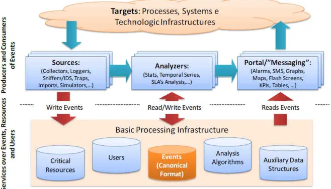
The background of this project is a large IT Company that has facilities and workers spread throughout the country, even if more concentrated in urban areas. To help monitor and manage its IT infrastructure, it deployed a Complex Event Processing [3] system named Pulso [4], that performs data acquisition, processing, transformation and display. Its architecture is depicted in Figure 1.

Figure 1 – Pulso complex event processing architecture

The Pulso system is composed of three kinds of entities. Data sources produce events that are sent and stored in the event repository, in a canonical format. Examples of data sources are active network probes, sniffers, application-generated events, etc. The analyzers process the raw events into higher-level events, extracting relevant information from data. Finally, the display entities

6

generate or display the available information into human-readable formats, like alarms, maps, graphs, tables, performance indicators, visual displays, web portals, etc.

The latest evolution of Pulso features workstation probes. These obtain flow information tagged with the source application and the account under which the application is executing. This kind of detail is rarely available, and it was the main drive for this project – to infer and group user behavior based on their tagged network flows.

2.2.

Dataset

For this project, a real dataset with two months worth of recent data, from April to June 2009, was made available. The dataset was obtained on a call center and contains tagged network flow information. A flow is defined in the usual way, the packets involved in a connection between a source and destination, usually characterized by the 4-tuple <source IP, destination IP, destination port, transport level protocol (TCP/UDP)>. The flows are tagged, and the tags contain the application that originated (or received) the flow, as well as the account under which it was launched. The information available for each flow is the start timestamp, the duration and total bytes transferred (per direction, and per transport protocol). Therefore, the information available are flow records of the kind <source IP, destination IP, destination port, transport level protocol (TCP/UDP), application, user account, start timestamp, duration, bytes transferred>. The information in bold is the one that is unique on this work, only available because of the workstation probes.

2.2.1. Dataset characteristics

The transformation from accounts to users is rather simple. Domain accounts translate directly into users. The remaining local accounts are related to system processes, and are designated System accounts. 0 100 200 300 400 500 600

3 Apr 10 Apr 17 Apr 24 Apr 1 May 8 May 15 May 22 May 29 May

Date # U se rs _System Users

7

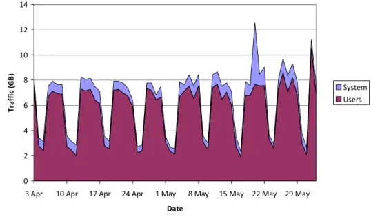
As it can be seen on Figure 2, the dataset has, on average, 160 distinct users per day on weekends and 490 on work days. A small percentage is system users. Figure 3 shows that total traffic averages from 3GB/day on weekends to 7GB/day on work days. System processes generate a little additional traffic. 0 2 4 6 8 10 12 14

3 Apr 10 Apr 17 Apr 24 Apr 1 May 8 May 15 May 22 May 29 May

Date T ra ff ic ( G B ) System Users

Figure 3 – Total daily traffic in dataset

In Figure 4, the number of distinct user flows is, on average, 55K/day on weekends and 130K/day on workdays. System processes increase these figures by 40%.

0 50 100 150 200 250

3 Apr 10 Apr 17 Apr 24 Apr 1 May 8 May 15 May 22 May 29 May

Date Fl o w s (K ) System Users

8

Ignoring all the system processes flows, the entire two month dataset has 1131 distinct users and 297 distinct applications (at the binary level). From these statistics, we can conclude that the dataset has enough size and information to be statistically significant.

2.2.2. Limitations

This dataset is all the information available to execute and evaluate this project, no additional information can be obtained. In addition, the probe system is already in place and cannot be modified. However, modifications and suggestions that result from this work can influence the next versions.

2.2.3. Pre-processing

‘Users’ are domain accounts that univocally correspond to human workers (there are no shared accounts). ‘System’ accounts refer to local workstation accounts related to OS tasks. By analyzing the data, system accounts were filtered from the dataset for two reasons. First, the applications that are directly run by users are more likely to mirror their behavior. After all, these are the ones they are interacting with. Second, system accounts will most likely be performing OS-relevant functions, and would generate noise for our analysis. Third, only a few tasks performed under system accounts might indirectly mirror human behavior, by being related to user applications. These are a minority, and this benefit is probably insignificant when compared to the noise they could add. For these reasons, they were filtered.

2.2.4. Classes

The user population was identified into three distinct ‘classes’ or categories. Note that in a single class there can be users from different departments. The three classes are:

• Class 0 – Callcenter Operators. These users have no special privileges, and should be performing a well-defined subset of tasks;

• Class 1 – Callcenter Supervisors. Supervisors monitor callcenter sections, and therefore have greater responsibility and privileges. Their tasks are less clear, since they have to solve all the problems that may arise;

• Class 2 – Others. This category includes users from tech support and specialized teams that may have administrative privileges and almost unlimited flexibility in the tasks they perform. The distribution from these classes is far from even; 90% are operators, 5% are supervisors and just 3% are others.

• Class 0 (Operators): 1035/1131 (91,5%)

• Class 1 (Supervisors): 60/1131 (5,3%)

9

2.3.

Data mining

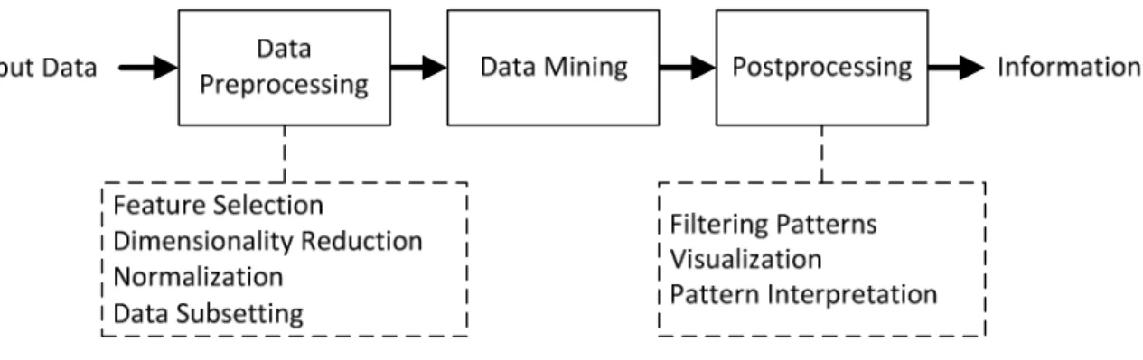
Data mining can be described as the process of extracting information from data. The main characteristic that tells it apart from traditional information retrieval techniques is the enormous sizes of the datasets. Traditional techniques may be unsuitable due, not only to this, but also because of the high dimensionality, heterogeneity and distributed nature of the data. To solve these problems, data mining is a confluence of areas, drawing ideas from machine learning, artificial intelligence, pattern recognition, statistics, and database systems. It is also related with Knowledge Discovery in Databases (KDD), the overall process of converting raw data into useful information. The steps of the KDD process, according to [5], are depicted on Figure 5. There are three main stages. The data preprocessing stage consists in reducing the available data to a manageable and meaningful set, i.e., selecting the relevant features, normalizing the data, etc. The data mining stage consists of extracting relevant information from this data set. The final stage may include manual tasks, and involves representing the relevant information into human-understandable form.

Figure 5 – Process of knowledge discovery in databases

The core data mining tasks are Clustering, Association Analysis, Predictive Modeling (Classification) and Anomaly Detection. These fall into two broad categories:

• Predictive tasks: Predict the value of some attributes (target variable) based on the value of other attributes (explanatory variables). Tasks in this category are Predictive Modeling (Classification) and Anomaly Detection;

• Descriptive Tasks: Derive human-interpretable patterns that summarize the underlying relationships in data. Clustering and Association Analysis are usually classified as descriptive tasks.

In the next section, we will first analyze the properties of data itself. Then, we will briefly discuss these tasks, with greater emphasis on the most relevant for our work.

2.3.1. Data

Evidently, data mining is about data. Data can be seen as a collection of data objects, each with a collection of attributes that characterizes it. The values the attributes can have depend on their type. Four properties are used to describe attributes, related with the operations than can be performed with them:

10

• Distinctness: = and ≠. With only these two operations, attributes can be either equal or different from one another.

• Order: <, ≤, > and ≥. These operations allow the values of an attribute to be ordered.

• Addition: + and –. These operations allow the values of an attribute to be added and subtracted.

• Multiplication: * and /. These operations allow the values of an attribute to be multiplied and divided.

With these properties, attributes are classified into four types. Each type contains all the properties of its predecessor:

• Nominal (distinctness). These attributes can only be compared against each other. Examples are ZIP codes, eye color, gender, etc.

• Ordinal (order and distinctness). These attributes also have a natural order, like happens with grades, street numbers, scales, the Mohs scale of mineral hardness, etc.

• Interval (addition, order and distinctness). These attributes can be added (and subtracted), which happens, for example, with calendar dates, temperature in Celsius or Fahrenheit.

• Ratio (multiplication, addition, order and distinctness). These attributes have an absolute zero value, and therefore can be multiplied (and divided), like what happens with age, mass, length, temperature in Kelvin, etc. Therefore, it makes sense to say, for example, that one person weighs twice as much as another person, but it makes no sense to say that a temperature of 20 Celsius is twice as warm as a temperature of 10 Celsius (because the Celsius scale has no absolute zero). However, on the Kelvin scale, 200 degrees can indeed be said to be twice as warm as 100 degrees.

It is also common to group nominal and ordinal attributes as categorical (or qualitative) attributes. Similarly, interval and ratio attributes can be labeled as numeric (or quantitative) attributes.

Nevertheless, the attributes can also be classified by a different property, the number of values they can have:

• Discrete attributes have a finite or countable infinite set of values. These attributes can be categorical, such as the examples before. Binary attributes are a special case of discrete attributes with just two values.

• Continuous attributes are those whose numbers are real attributes.

Both of these classifications are important because most techniques can only handle certain type of attributes, and it is common to refer to them by any of these classifications.

Data sets

All data sets have three characteristics that have a significant impact on the data mining techniques that can be used: dimensionality, sparsity and resolution.

11

The dimensionality of a data set is the number of attributes that the objects in that data set possess. The difficulty in analyzing high-dimensional data is referred as ‘the curse of dimensionality’. To solve this, dimensionality reduction techniques are used, and some will be discussed later.

Sparsity relates to the ratio of the dataset object attributes that have a non-zero value over the entire data set object attributes. If this ratio is low, the dataset is labeled sparse. In practical terms, this is an advantage since usually only the non-zero attributes have to be stored and manipulated. Resolution influences the size of the dataset, and, consequently, which properties will be discernible, i.e., the patterns on data depend on the level of resolution. If the resolution is too high, the pattern may be hidden in noise, if it is too low, the pattern may disappear altogether. For example, a document scanned at 100 dpi is smaller, and may allow individual characters to be recognized. The same document scanned at 100 times that resolution, 10K dpi, will be much larger. The type of printing technology and paper texture can be discerned, but the fact that it contains text may not be detected.

Dimensionality reduction techniques

Principal Component Analysis (PCA) [6] and Singular Vector Decomposition (SVD) [7] are two widely used techniques for dimensionality reduction. PCA differs from SVD in the fact the PCA removes the mean of the data and SVD does not.

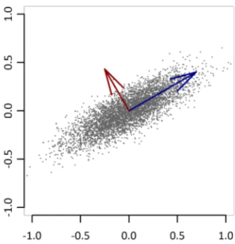
Both involve a mathematical procedure that transforms a number of possibly correlated variables into a smaller number of uncorrelated variables called principal components. The first principal component (dimension) tries to capture as much of that variability as possible. The second dimension will be orthogonal to the first, captures as much of the remaining variability, and so on. The resulting set of dimensions constitute a new multidimensional space where the original data is projected. The idea is to capture as much of the variability of the data as required in a lesser dimensional space. The original dataset can then be projected into this reduced-dimensionality space. Since it has fewer dimensions, it is likely that more data mining algorithms can be applied to the data set. Note that in the end of processing, the data can be projected back into the original space, where it has meaning.

12

Take Figure 6 as an example. The two vectors clearly point to the directions of greater variability. If that space had to be reduced to just one dimension, the longest vector could be used, and a projection on that (uni-dimensional) space would account for most of the variability.

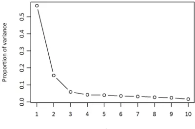
Another common visualization method related with dimensionality reduction is the scree plot, shown in Figure 7. A scree plot shows the relationship between the principal components and the variance explained by each of them. They are sorted by explained variance (Y-axis), and the X-axis contains the principal components. A scree plot helps the analyst visualize the relative importance of the principal components (also called factors) — a sharp drop in the plot indicates that subsequent factors are ignorable, because they explain less variability. In Figure 7, the most important components are the first two, because they are clearly higher than any of the others. It is also common to select the principal components up to the ‘knee point’ of the curve.

Figure 7 – Scree plot

In short, PCA has some interesting characteristics:

• Tends to identify the strongest patterns in the data. Can be used as pattern finding technique;

• Often, most of the data variability can be captured by a small fraction of total dimensions. After this dimensionality reduction, low-dimensionality techniques can be used;

• If the noise is weaker than the patterns, dimensionality reduction can eliminate much of the noise.

2.3.2. Clustering

The goal of cluster analysis is to divide data into groups (clusters) that are meaningful and/or useful. For that, the clustering algorithm needs a similarity measure, a function that calculates the degree to which two objects are alike. The Euclidean distance is a very simple and popular similarity distance for continuous attributes, but there are others, like the Mahalanobis distance, the cosine similarity or the Jaccard coefficient.

13

Any clustering algorithm will try to group data points such that intra-cluster similarity is maximized and inter-cluster similarity is maximized. In other words, create clusters such that data points in one cluster are more similar to one another and data points in separate clusters are less similar to one another.

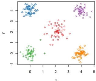
Consider the example in Figure 8. The algorithm used the Euclidian distance as its similarity measure, so the idea was to group points that were close to one another. The data set was grouped into five groups, indicated by the different shapes (and colors). The goal was achieved, as five distinct groups are evident.

Figure 8 – Clustering example

Next, three clustering algorithms will be presented: K-means, X-means and DBScan.

K-means

K-means [8] is one of the oldest and most widely used clustering algorithm. It is a prototype-based clustering algorithm that can be applied to objects in a continuous n-dimensional space. In prototype-based clustering algorithms, a cluster is a set of objects that is closer (more similar) to the prototype of that cluster, than to the prototype of any other cluster. In K-means, the prototype is the centroid, i.e., the mean of a group of points. The algorithm, quite simple, is shown on Table 1.

1. Select K points as the initial centroids 2. Repeat

3. Create K clusters by adding the points to its closest centroids 4. Recalculate the centroids for each of the K clusters

5. Until the centroids do not change

Table 1 – K-means algorithm

Despite its simplicity and effectiveness, it is not without issues. First, K (the number of clusters) has to be manually specified beforehand. In addition, the selection of the initial centroids affects the outcome of the algorithm. The algorithm may converge to a local minimum, and not to a global minimum. Several workarounds can be used, like randomly generating centroids, running that algorithm multiple times and choosing the best run (the one with less total error). A better approach is the one used in X-means, which we will analyze in the next chapter.

14

K-means does have modest time and space requirements. Let m be the number of points, n the number of features and t the number of iterations to converge. Its space complexity is O((m+K)n), because only data points and centroids are stored. Time complexity is O (t*K*m*n), but since t is usually small, and if K<<m, it will be linear with m. In short:

• K-means strengths: Simple, efficient, even with multiple runs;

• K-means weaknesses: Not suitable to all types of data: non-spherical clusters or clusters of different sizes and densities; has trouble clustering data with outliers, although outlier detection and removal can help.

X means

X-means [9] is a Carnegie Mellon evolution of the popular K-means algorithm that addresses two of its shortcomings: it improves computational scalability and determines an ‘optimal’ number of clusters K. This algorithm is much faster than repeatedly using K-means for different values of K, a common practice for automatically determining K. The computational scalability improvements are due to the data structure used (multiresolution kd-trees, a special case of BSP-trees) and blacklisting (considering only the needed centroids for each region).

The optimum K is determined by recursively splitting each centroid into two or more, and evaluating if the resulting subclusters are better than the single one – a technique known as bisecting K-means. The algorithm uses the Bayesian Information Criterion (BIC) scoring function as its optimal measure. Nevertheless, it still requires a range of K ([kmin, kmax]) as input to determine the optimum K.

DBScan

DBScan [10] is a density-based clustering algorithm. These algorithms locate regions of high density that are separated from one another by regions of low density. The density of a point is the number of points inside a radius Eps (a configurable parameter). The results of this type of algorithm depend heavily on Eps. Consider the extreme cases: If Eps is too large, the density will equal m, i.e., all points are within Eps. On the other hand, if it’s too small, the density will equal 1 (only that point is within Eps).

The algorithm, shown in Table 2, uses three types of points:

• Core Points are the ones in the interior of a cluster. A point is considered a core point if the number of points inside Eps exceeds a threshold MinPts (the other configurable parameter).

• A Border Point is a point that is not a core point, but is in the neighborhood of at least one border point

• Noise points are all the others, i.e., points that are neither core nor border. 1. Label all points as core, border or noise

2. Eliminate noise points

3. Create an edge between all core points within Eps of each other 4. Make each group of connected points a separate cluster

5. Assign each border point to one of the clusters of its core points

15

Let m be the number of points. Time complexity of DBScan is O(m*time to find points in the Eps neighborhood). The worst case is O(m2), but using kd-trees and in low-dimensional spaces it can be O(mlog(m)). Space complexity is just O(m), since only small amount of data is kept for each point: cluster label and type (core, border, noise). Summing up:

• DBScan Strengths: Classifies points as outliers, not all have to forcibly belong to a cluster; for the same reason, it’s resistant to noise; handles clusters of arbitrary shapes and sizes;

• DBScan Weaknesses: Does not handle well clusters with widely varying densities; it also does not handle well high-dimensional data, since density is more difficult to define; expensive when computing nearest neighbor requires computing all pair-wise proximities, as it is high-dimensional data.

2.3.3. Predictive modeling (classification)

Classifiers require a collection of records (designated a training set), where each record contains a set of attributes, and one of the attributes is the class. The purpose of a classifier is to classify previously unseen records (assign a class) as accurately as possible. That is accomplished by finding a model for the class attribute as a function of the values of other attributes, i.e., class = f(attribute1,

attribute2, …, attributen). To determine the accuracy of the model, test sets (previously unseen

records) are used. Usually, a given data set is divided into training and test sets, with the training set used to build the model and test set used to validate it.

Classification techniques are most suited for datasets with binary or nominal categories and less effective for ordinal categories. There are many techniques for building classifiers, each resulting in a different type of model: decision trees, rule-based, nearest-neighbor, Bayesian, artificial neural networks, support vector machines, ensemble methods, etc.

Classifiers are evaluated based on metrics derived from its classification accuracy. This means that some of the models are not designed to be easily interpreted by humans, and use the black box approach, in the sense that no information can be extracted from them. Neural networks are an extreme example of that.

2.3.4. Anomaly detection

The idea behind anomaly detection is simple: find objects that are different from most other objects. A variety of approaches exist, all trying to capture the idea that an anomalous object is unusual or in some way inconsistent with the other objects. The three main approaches for anomaly detection are:

• Model-Based – Build a model, anomalies are the ones that don’t fit well into the model;

• Proximity-Based – Anomalous objects are distant from most other objects;

• Density-Based – Objects in low density regions are relatively distant from their neighbors and can be considered anomalous.

Class labels are labels that indicate if a data point is anomalous or normal. Considering the class label requirements, each technique can be classified as supervised, unsupervised and semi-supervised.

16

Supervised anomaly detection requires a labeled training set with both anomalous and normal objects. In unsupervised anomaly detection, no class labels are available. On semi-supervised, only normal labels are available in the training set (no anomalous labels).

Chandola’s recent and thorough survey on anomaly detection [11] is a new reference in this area, much more complete than the previous overviews, for example, Patcha [12]. Patcha’s was more focused on Intrusion Detection, while Chandola’s covers a broader spectrum of applications. Note that anomaly detection is not our primary goal, and, therefore, not all techniques are available to us. Classification-based anomaly detection involves training a classifier with normal (or abnormal) data, so that it can recognize (classify) anomalies. However, most of the classifiers require supervised data in the training phase, i.e., the supplied data must be labeled (as ‘normal’ behavior, or as ‘abnormal’ behavior). Nearest-neighbor techniques assume that normal data instances occur in dense neighborhoods, while anomalies occur far from their closest neighbors. These techniques (distance to kth nearest neighbor and relative density) are somewhat similar to the ideas behind clustering. Clustering-based anomaly detection is of particular interest, since we are grouping similar behavior into clusters. The available techniques rely on one of three basic assumptions:

A1: Normal data instances belong to a cluster, while anomalies do not. Under this assumption, any clustering algorithm that does not forcibly cluster all elements can be used, like DBSCAN. A disadvantage of these techniques is that they may not be optimized for finding anomalies, since their main aim is to find clusters.

A2: Normal data instances lie closer to their centroids than anomalies. Techniques that rely on this assumption first use any clustering algorithm, and then, the distance to its closest centroids is its anomaly score. K-means clustering, Expectaction-Maximization and Self-Organizing Maps (SOM) have been analyzed by Smith et al. in [13].

One weakness of this approach is that if the anomalies form clusters by themselves, these techniques will not detect them. In other words, anomalous clusters are not detected. To tackle this problem, a third category of clustering based techniques has been used, which relies on the following assumption:

A3: Normal data instances belong to large and dense clusters, while anomalies either belong to small or sparse clusters.

Although not considered by the authors, if the number of clusters is acceptable and human-understandable, manual classification can be a perfect detector of such anomaly clusters.

Statistical anomaly detection is also worth mentioning. The underlying assumption is that normal data instances occur in the high probability regions of a stochastic model, while the anomalies occur in the low probability regions. These techniques fit a statistical model to the data, and then apply a statistic inference test to determine the probability of an instance belonging to the model or not. Parametric techniques assume that the normal data is generated by a parameterized parametric distribution. Non-parametric techniques do not require that the model is known a priori, it is defined from the data. These techniques typically make fewer assumptions regarding the data.

17

Histogram-based techniques construct histograms to maintain a profile for each attribute of the data. Kernel function based techniques use a function to estimate the actual probability density function. Parzen windows estimation [14] is a known and proven function. Note that kernel-based techniques can potentially have quadratic time complexity in terms of data size.

2.3.5. Association analysis

The goal of association analysis is, given a set of records each of which contain some number of items from a given collection, to produce dependency rules which will predict occurrence of an item based on occurrences of other items. This area first originated to deal with customer purchase data, designated market basket transactions.

Transaction ID Items

1 {Bread, Milk}

2 {Milk, Apples, Juice, Cola} 3 {Bread, Milk, Apples, Juice} 4 {Bread, Milk, Apples, Cola} 5 {Apples, Bread, Eggs, Juice}

Table 3 – Market basket transactions example

For example, considering the transactions on Table 3, it might be concluded that {Bread} -> {Apples}, i.e., clients that buy bread are very likely to buy apples. This exemplifies the type of conclusions that can be drawn from association analysis. A very important aspect of these algorithms is that they only consider sets of categorical data, resulting in binary attributes. That is, the amounts of each item of a set are ignored. This has an impact on which domains these techniques can be applied.

2.4.

Related work

Our work is a novel approach that applies existing and proven techniques towards a new goal, user network behavior analysis. Evidently, it is a multidisciplinary project that builds on several relevant fields, namely, traffic classification, data mining and user behavior. The related works are grouped by their major field, and analyzed in the next subsections.

2.4.1. Traffic classification

The goal of traffic classification is to identify and/or categorize network traffic, by analyzing some of its properties. The most common goal is to determine which application generated that traffic. While this is clearly not the main goal of this project, since the type of traffic and even the application is already known, this area of research is very relevant. The techniques and methods used to group and classify traffic are the foundation for grouping the users, since our working data consists of network data flows.

Botminer [15] is a botnet detector using network traffic. Although the goal is quite different from our own, the techniques used are very interesting and similar to the ones we developed. Under the assumption that bots within the same botnet are likely to behave similarly, the technique involves clustering hosts using features of their behavior. First, flows are grouped into <source ip, destination ip, destination port, protocol (tcp/udp)> groups, per day. The relevant attributes considered are

18

number of flows per hour, number of packets per flow, average bytes per packet, and average bytes per second. Afterwards, for each of these four random variables, an approximate version of their distribution is computed by binning – dividing the entire sample set into groups of interval ranges, called bins. However, instead of using fixed-size binning, n quantiles between 5% and 90% are computed, and their values used as the bins limit. The last bin will contain all samples greater than the last quantile (90%). In effect, this technique is providing variable-sized bins, maximizing the information retained by the approximation.

Clustering is performed in two steps. Since the previous binning technique generates many dimensions (number of bins * number of attributes), and the datasets also have high cardinality, a first, coarse-grained clustering is performed. For dimensionality reduction, only the mean and variance of the each distribution is used. Afterwards, for each cluster, a second clustering step is performed, this time with all the dimensions. The clustering algorithm used is X-means. Also noteworthy is the fact that two different data sources are used and clustered (network flows and activity). Afterwards, the clusters are correlated, and each host will receive a high score if it has performed multiple suspicious activities, and if other hosts in the same cluster exhibit the similar behavior.

In [16], Erman et al. used clustering algorithms to perform traffic classification using only traffic statistics at the transport layer level. Classification techniques using transport-layer statistics rely on the fact that different applications typically have distinct behavior patterns when communicating on a network. For example, a large FTP file transfer would have a larger connection duration and packet size than an instant-messaging client sending sporadic short messages to other clients. Clustering analysis is one of the methods for identifying classes among a group of objects. They compared K-means, DBSCAN and AutoClass algorithms on two empirical packet traces. For evaluation, the ratio of true positives over number of samples was used. Autoclass achieved the best accuracy, but only by a small margin, and it is almost two orders of magnitude slower than the other two. This factor also limits the number of samples it can handle in a reasonable amount of time. DBSCAN had the highest precision (ratio of true positives to false positives), and has the ability to label samples as noise.

BLINC [17] (BLINd Classification) uses a different approach to traffic classification. Instead of classifying individual flows, it associates hosts with applications and then classifies their flows accordingly. The argument is that observing the activity of a host provides more information about the nature of the applications of that host. Note that BLINC only classifies hosts according to 11 categories; it does not identify individual applications. Nevertheless, it does not use payload information or well-known port information. The behavior of each host is captured at three levels: social, network and application.

The social level captures the interaction with other hosts, and its popularity (the number of other host it communicates with). This is used to detect groups, or, communities of nodes, which are hosts that interact with each other. This grouping is performed using cross-association algorithms.

At the functional level, it is determined if a host is a provider or a consumer of a service, or if it participates in interesting communities. This is done by using the number of source ports a particular host uses for communication. A server is likely to use a single source port in most of its flows, while a client is more likely to use many (ephemeral) source ports.

19

The application level captures transport layer interactions and the final classification is refined. The host behavior is captured by matching all the levels against a library of empirically derived patterns, called graphlets. It is not mentioned how these patterns are derived, but it is highly likely a manual task, which is disappointing.

In conclusion, BLINC is a complex multilevel classification approach that has a reasonable level of accuracy and completeness.

Roughan et al. proposed a statistical signature-based approach [18] to solve the traffic classification problem. The purpose was to classify traffic into a reduced set of classes (interactive, bulk data, streaming and transactional). For each class, few applications (typically one) were chosen to train the model, using supervised learning, a predictive modeling technique. The methods considered were K-Nearest Neighbor and Linear Discriminant Analysis. The most relevant traffic features used in the model were average packet size and flow duration. Nevertheless, the authors had to include an additional feature, packet inter-arrival variability, to more accurately distinguish streaming traffic from data transfer traffic. Using 10-way cross-validation for evaluation, the results error rate was under 10% for the training applications, but higher for new applications. It seems that more work needs to be done.

In ACAS [19], Haffner et al. also tackled the traffic classification problem by creating signatures. However, their goal was to determine which application a flow belongs to by inspecting application layer information only (payload). Using supervised learning techniques (Naïve Bayes, AdaBoost and Maximum Entropy), each classifier was trained using labeled data. Results showed that the first 64 bytes of each flow were sufficient to classify the seven applications analyzed with a maximum error not exceeding 0.6%. Two of the applications were encrypted streams, namely https and ssh. In short, ACAS is using machine-learning techniques to distinguish the header of each flow.

What is interesting in ACAS is the technique used to convert the payload data. Since these classifiers are known to perform well on binary data, a discrete byte encoding technique was used to convert the payload data into binary features. The first n-bytes of a flow f are converted into a feature vector v with n*256 elements. The value of each byte sets the value of the corresponding vector position to one. All the others remain at zero. This encoding also has the important property that all byte values are equidistant (based on the Euclidean distance). That is, each byte value is either equal (distance=0) or different (distance=1) from each other. If the first n-bytes of f were used directly, for example, byte values 23 and 25 (distance=2) would be considered closer (more similar) than byte values 50 and 80 (distance=30). This would introduce an unwanted bias in the results.

The problem that Tan et al. address in [20] is different; the goal was to group hosts into similar groups, based on their connection patterns. The number of connections is not used, only the fact that a host has contacted another. The grouping problem was solved by reducing it to a bi-connected component graph problem. However, the interesting part was that the number of groups produced was deemed too large. A subsequent phase reduced the number of groups by merging groups that where similar, according to the similarity function and number of connections. This phase had tuning parameters that had to be set to produce the desired results. Also noteworthy, was the notion of identifying group evolution over time. That is, groups formed by subsequent runs of the algorithms may have different ids, while being functionally the same. This role correlation

20

algorithm allowed tracking group variations over time. This is an important issue and solution, as grouping algorithms not always generate groups with the same id.

2.4.2. Data mining

The work by Moore, Han et al. on [21] deals with many of the challenges that we also faced, namely, when the dimensionality of the feature space becomes high relative to the size of the document space. The domain was to categorize web pages and extract the most relevant features (in this case, words). One of the methods is ARHP [22], which uses association rules discovery and hypergraph partitioning. The other one is Principal Component Analysis (PCA) Partitioning Algorithm, which cuts the space of documents with a hyperplane passing though the arithmetic means of the document and normal to the principal direction. The process is repeated recursively, creating a tree like hierarchy along the principal vectors. The algorithms were compared using an entropy measure, and both methods performed better than the traditional clustering algorithms analyzed: AutoClass and Hierachical Agglomeration Clustering (HAC).

However, a more detailed analysis and their subsequent work on [23] clarifies that their model is suited towards frequent itemset mining, and not “clustering” in the traditional sense. More importantly, their scheme does not naturally handle continuous variables, which is the type of data we have on our work. They did develop a new algorithm called Min-Apriori [24] that operates directly on continuous variables without discretizing them. However, it is not clear if this variation was used in more recent works, like PACT [25].

Henderson et al. focused on analyzing user behavior in networked games [26], namely, Half-Life, Quake and Quake 3. Some results were expected, for instance, the number of players exhibit strong seasonal (time-of-day) variation. Player’s session duration time fit an exponential distribution, and interarrival times fit a heavy-tailed distribution. In addition, the number of players in a session affects new players’ decision to join or not a server, corroborating the empirical idea that players do not want to join empty servers. Also interesting were the techniques used for the analysis. The temporal autocorrelation function (ACF) and ARIMA (Autoregressive Integrated Moving Average) models [27] were used to examine these network externality effects.

Park and Giordano use anomaly detection to detect insider threats in [28]. They define the users’ behavior using frequency patterns of their system actions (Search, Send, Copy). Then, as users have roles assigned to them, a pattern is inferred for each role. To detect anomalies, their technique involves two facets: role-level comparison, and individual comparison. Role-level comparison, matches each user’s behavior against that of its role (spatially). Individual comparison matches each user’s behavior against their own behavior while performing the same tasks in the past. Unfortunately, the implementation used a controlled simulation with synthetic data sets. Nevertheless, this dual-base comparison (against the group, and against the past) is quite interesting.

The work by Lakhina in [29] is relevant, because of the usage of PCA for network traffic flows analysis. This was an example of using PCA to solve the “curse of dimensionality”. The analysis involved analyzing origin-destination flows over time in a network. In the datasets considered, there were fewer than two hundred dimensions. This is a high value, but not as high as the one we came across in our model. Nevertheless, just between 5 and 10 principal dimensions were enough to

21

accurately approximate the network flows. Another interesting conclusion was the classification of the eigenflows (network flows projected in some principal components) in three distinct categories: seasonal, spike and noise. In addition, the low-coordinate space formed by PCA shows some evidence of stability over time.

InteMon [30] is a monitoring system that uses PCA to automatically infer correlations between data streams and alert when those correlations break. The system uses energy thresholding to automatically select the number of dimensions required to represent the data. An anomaly is signaled when the number of dimensions changes, indicating that either a correlation was broken, or a new one was created. Also noteworthy is using the reduced dimensional space obtained by PCA of the original streams to considerably reduce the sensor data storage space requirements. InteMon is a real-time monitoring system, so it uses a stream mining algorithm to perform PCA named SPRINT [31].

2.4.3. User behavior

In [32], Manavoglu et al. present a sequential model for learning individualized behavior models for web users. First, a global behavior model is built for the entire population. Each component of the mixture model represents a dominant pattern in the data, and each sequence (user session) is modeled as a weighted combination of these components. Then, it is personalized by assigning each user individual component weights for the mixture model. They concluded that the Markov model performed better for predicting the behavior of known users, where the maximum entropy (maxent) model was better at the global behavior model (and also unknown users). Note that the maxent model was only computational feasible because of the reduced dimension of the action space. Mobasher et al. goal in [25] was to discover aggregate usage profiles to use as input source for recommender systems. In order to find overlapping aggregate profiles, two techniques were used: clustering of user transactions and clustering of pageviews. The relevance of this work is the experimental evaluation of the aforementioned profile discovery techniques based on real usage data. The first algorithm, PACT, uses standard clustering algorithms (K-means was used) to partition the space in groups of transactions that are close to each other according to some distance measure. A transaction is an n-dimensional vector in all the pageviews space. The aggregate profiles are generated from the centroids of each group. For each cluster c, a mean vector is computed by finding the ratio of the sum of the pageview weights across transactions in c to the total number of transactions in the cluster. The weights are then normalized, and low-support pageviews filtered out. PACT is similar to method proposed by Karypis and Han in [33], but applied to transactions and not documents.

The second method clusters pageviews across user transactions. The idea is to capture overlapping interests of different types of users. However, since the transactions are now used as features, traditional distance-based techniques cannot be used because there are hundreds of thousands of dimensions. In addition, dimensional-reducing techniques may not be appropriate, as they may discard too much information. Instead, the Association Rule Hypergraph Partitioning (ARHP) [23] technique was used, using the well-know Apriori [34] algorithm.

The authors concluded that PACT was the overall winner in recommendation accuracy, but Hypergraph does better when focused on more restricted data. Hypergraph produced a smaller set

22

of high quality and more specialized recommendations. On the other hand, PACT has a performance advantage when dealing with all the relevant data.

23

3

Model and architecture

3.1.

Architecture

We followed an incremental approach and opted for a modular architecture. This enables each module to be replaced, upgraded, and even developed without affecting the rest of the system. It also creates a testbed to compare different approaches to solve each of the problems. The architecture is depicted in Figure 9.

Figure 9 – Architecture block diagram

The first stage, data generation, is executed by Pulso, as described in section 2.1, using the workstation probes and data collection mechanisms. This was the process used to create the dataset. Note that even this part of the process can be replaced with another that produces similar (or even different) data.

The profiler is responsible for interfacing with the data, so it has to execute the pre-filtering operations. Its goal, however, is to characterize each user’s behavior according to a model. This tremendously reduces the data size to a manageable level, while remaining useful for the other blocks. Afterwards, the roler will gather all the individual user profiles and group them into roles with similar behavior. Each role will characterize a different type of behavior. The anomaly detector, by comparing the individual user patterns with the available roles will determine which ones have the highest probability of being anomalous behavior. We will now discuss each component in detail.

3.2.

Profiler

First, the profiler has to interface with the database where the dataset is stored, adapt and convert the data to a manageable format and pre-filter it. As mentioned before, for this dataset it means to filter out local accounts. Next, the goal is to characterize each user behavior by using tagged flow information. The challenge is how to balance the tradeoffs. On one hand, the profile has to be

24

specific enough so that the roler can detect similar behavior, and the anomaly detector can detect anomalies. On the other hand, the profile size must be much smaller than original sample size – so that all components can run in acceptable time (i.e., solve the dimensionality problem). In addition, it must scale, so that it can be applied to bigger data samples. The solution is to choose an adequate model that satisfies all these properties. The task of the profiler then becomes to transform the original data into the model format, creating the user profile.

3.3.

User profile model

Recalling our dataset information, for each user, there are three attributes of flow information per application: start timestamp, duration and total bytes transferred. Since the innovation of this dataset is the application information, ideally, we would want to characterize the user’s behavior using each application. For each relevant attribute, one could capture, for example, the average, the variance and any other number of statistical moments. However, that approach not only throws away too much information, as it is difficult to interpret and explain. For example, average and variance may have some empirical meaning, but what about skewness (asymmetry of the probability distribution), kurtosis ("peakedness" of the probability distribution), and the subsequent statistical moments? We propose a different approach, where we instead use a discretization of the probability density function.

In statistics, the probability distribution (or density) function of a random variable is a function that describes the density of probability at each point in the sample space. The probability of a random variable falling within a given set is given by the integral of its density over the set. We propose a discrete version of this concept, defining a stepwise function with a fixed number of slices. The function is built from the corresponding histogram. This way, we retain most of the sample’s relevant features, as a tradeoff with space. The configurable tradeoff parameter is r, the number of slices. Therefore, we construct a discretized probability distribution function (pdf) in the following manner:

1) Define the resolution r – the number of bins (or slices);

2) Split the sample space into sequential non-overlapping intervals, and assign each bin to an interval. Every point in the sample space must be covered by one, and only one bin;

3) All bins are initially empty, and each has an associated counter, with is initialized to zero; 4) For each sample in the set, determine the corresponding bin to which it belongs, and

increment its counter value;

5) Normalize each bin counter, so that the total area is 1. In other words, divide the value of each bin counter by the total number of samples across all bins;

6) Define a function pdf(s) that for each input of s, returns the corresponding normalized bin count. s must be in the range {1,2,3,…,r-1,r}.

For example, let’s consider total traffic from individual flows. Each sample is the total traffic (in KB) from a distinct flow. The sample set will be {2,6,8,9,11,14,17}, i.e., 7 distinct flows. Let’s set