Rainer Haldenwang
[email protected] Cape Peninsula University of Technology Civil Engineering 8000 Cape Town, South AfricaReinhardt Kotzé
[email protected] Cape Peninsula University of Technology Civil Engineering 8000 Cape Town, South AfricaRaj Chhabra
[email protected] Indian Institute of Technology KanpurDepartment of Chemical Engineering Kanpur, India
Determining the Viscous Behavior of
Non-Newtonian Fluids in a Flume
Using a Laminar Sheet Flow Model
and Ultrasonic Velocity Profiling
(UVP) System
The flow of non-Newtonian fluids in rectangular open channels has received renewed interest over the past number of years especially as large flumes are being used to transport tailings in countries like Chile. The effect of yield stress on the flow behavior is complex and not yet fully understood. The Ultrasonic Velocity Profiling (UVP) technique has been used to construct velocity profiles of non-Newtonian fluids flowing in a 10 m by 300 mm wide tilting flume. The contour maps were integrated to show that the velocity profiles were indeed correct. The thin film flow models available in the literature have been tested in terms of flow depth and Reynolds number. The measured profiles also show the influence of the side walls on the general flow features as the distance from the centre increases. The results reported herein span the laminar, transition and turbulent flow regions. As far as can be ascertained, it is the first time that this technique has been used to measure velocity profiles in opaque non-Newtonian fluids for open channel flow. It is shown here that, under appropriate conditions, the velocity profile and flow depth can be used to obtain the viscous properties of the fluids tested. Excellent correspondence between the rheological parameters inferred from the velocity profile measurements and that from the tube viscometry was obtained.
Keywords: open channel, ultrasound velocity profiling, sheet flow, non-Newtonian fluid, rheology
Introduction1
In recent years, there has been a renewed interest in studying the flow behavior of non-Newtonian fluids in open channels and flumes. Interest in such studies stems from both theoretical and pragmatic considerations. For instance, satisfactory understanding of thin film flow is germane to ensuring uniform product quality in scores of coating applications like in food and paper making applications. Further relevant applications are found in personal care products like in tailoring the rheological properties of creams, lotions and sun screens for their satisfactory end use (Laba, 1993). On the other hand, open channel or free surface flows are frequently encountered in the mining industry where flumes or launders are used routinely to transport mineral slurries and mine tailings for their disposal (Fuentes, 2004; Fernandez et al., 2010; Alderman and Haldenwang, 2007). Further applications abound in the lava and geological flows. Finally, this model configuration also has potential of being relevant in the evaluation of rheological characteristics, especially steady shear stress– shear rate of time-independent fluids, e.g., see (Chhabra and Richardson, 2008; Astarita et al., 1964). The bulk of the literature on this subject has been summarized recently (Haldenwang et al., 2010) and therefore only the key points are recapitulated here.
The currently available body of knowledge on this subject is conveniently classified into three sub-categories. The earliest analyses are based on the assumption of one-dimensional, laminar, fully developed flow on an inclined plane surface. In spite of their idealized nature, this class of solutions has often served as a convenient tool to extract the value of the rheological parameters simply from inclination versus flow rate data. While this has proved to be a useful rheological information tool, the limits of the validity of the one-dimensionality, etc. are not yet known (De Kee et al., 1990). The second sub-category of studies in this field endeavors to develop friction factor-Reynolds number plots akin to the Moody
Paper received 6 August 2011. Paper accepted 16 April 2012 Technical Editor: Monica Naccache
plot for different kinds of purely viscous non-Newtonian fluid models such as the power-law, Bingham plastic and Herschel-Bulkley model, etc. While the laminar flow is amenable to theoretical analysis based on the assumptions of one-dimensional, steady flow, extension to the flow conditions beyond the laminar flow regime is often based on dimensional considerations aided by experimental observations (Chhabra and Richardson, 2008; Haldenwang et al., 2010 and Kozicki and Tiu, 1967, 1986). Similarly, owing to the thin film approximation inherent in such studies, it is not always justified to overlook the influence of the morphology of the solid surface (Haeri and Hashemaabadi, 2009).
J. of the Braz. Soc. of Mech. Sci. & Eng. Copyright 2012 by ABCM July-September 2012, Vol. XXXIV, No. 3 / 277 Theoretical Considerations
De Kee et al. (1990) considered the one-dimensional, laminar, steady and fully developed gravity driven flow of time-independent non-Newtonian fluids down (Fig. 1) an inclined plane which is very wide in the other two directions. They approximated the steady shear rheological behavior by the well-known Herschel-Bulkley fluid model written in simple shearing motion as:
n xz y xz
τ = +τ K(γ& ) (1)
On the other hand, the application of the Cauchy’s momentum equations yields the following linear dependence of the shear stress on the x-coordinate as:
ρgxsinα
τxz = (2)
The maximum shear stress occurs at the wall and is given by:
ρghsinα
τ0= (3)
Owing to the presence of the yield stress, τy, it is fair to
anticipate that there would be a plug-like region near the free surface, as shown schematically in Fig. 1. If this region extends up to x = x0, the velocity of the plug will be constant in the region 0 ≤ x
≤ x0. Beyond x ≥ x0, the velocity will progressively decrease from
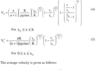
the plug velocity to a zero value at the wall due to the no-slip condition. By combining these equations, De Kee et al. (1990) derived the following formulae for the point velocities as well as the average velocity. − − − − + = + + + n 1 n 1 τ τ 1 τ τ 1 τ τ 1 K τ ρgsinα
K 1 n n V y 0 y n 1 n 0 y n 1 n 0 Z (4)
For
x
0≤
x
≤
h
(
)
+ + < − + = n 1 n 0 y n 1 n 0 z τ τ 1 K τ ρgsinα 1 n nK V (5)For
0
≤
x
≤
x
0The average velocity is given as follows:
(
)
τ τ + + τ τ − τ α ρ + = + + 0 y n 1 n 0 y n 1 n 0 1 n n 1 1 K sin g 1 n 2 nKV . (6)
In the present work, the nature of the flow was delineated by evaluating the Reynolds number proposed by Haldenwang et al. (2002) and Haldenwang and Slatter (2006) as written here for the flow of Herschel-Bulkley model fluids:
n h y 2 H R 2V K τ V ρ 8 Re + = (7)
Note that Eq. (7) includes the limiting cases of power-law fluid (τy = 0), Bingham plastic fluid (n = 1) and Newtonian fluids (n = 1
and τy = 0). In this work, the limit of the laminar flow region where
transition starts was deemed to occur at a point where the data began to deviate from the 16/Re line on the Moody Diagram. The hydraulic radius Rh for a rectangular channel is evaluated as
follows: 2h W Wh P A Rh + = = (8)
It is also appropriate to mention here that the standard dimensional considerations will yield a Reynolds number:
2-n n h V R Re k ρ =
and an Oldroyd number:
y n h Od V k R τ = .
It is readily seen that the Reynolds number,Re , given by Eq. (7) H
combines these two parameters into one as:
H
Re Re
1 Od
=
+ β , (9)
where
β
is a numerical constant. A similar composite Reynolds number has also been found to be successful in reconciling the drag data of falling spheres in visco-plastic fluids (Chhabra, 2006).Figure 1. Schematic of flow configuration (De Kee et al., 1990).
Experimental Methods and Materials
UVP-PD method for in-line rheological characterization
profiles in opaque liquids in research and engineering and it has been previously applied in complex geometries such as stirred tanks (Bouillard et al., 2001; Ein-Mozaffari and Upreti, 2009), contractions (Ouriev and Windhab, 2003; Kotzé et al., 2011), liquid metal target of neutron spallation source configuration (Takeda and Kikura, 2002), cylindrical hydrocyclone (Bergström and Vomhoff, 2004) as well as diaphragm valves (Kotzé et al., 2011). This highly versatile technique can also be used to determine fluid properties such as concentration profiles (Sad Chemloul et al., 2009), solid particle velocity as well as rheological properties.
Steger (1994) and Muller et al. (1997) developed the so-called Ultrasonic Velocity Profiling with combined Pressure Difference (UVP-PD) method where the measurement of pressure drop was added to the measured velocity profile to obtain rheological data. Based on this idea, Ouriev (2000) developed an in-line UVP-PD system for in-line measurement of the rheology of complex fluids. Birkhofer (2007) and Wiklund (2007) further optimized and/or refined the system. Kotze et al. (2008) successfully employed this method for the flow of highly concentrated opaque mineral suspensions in circular pipes. They reported a good agreement (within 15%) between the rheological parameters extracted from the detailed velocity profiles and those obtained from tube viscometry.
Flume rig
The test work was carried out in a 10 m long tilting flume, as detailed elsewhere (Haldenwang 2003; Haldenwang & Slatter, 2006). In brief, it consists of a 10 m by 300 mm wide tilting flume, which can tilt from horizontal by up to 5 degrees. The flume is linked to an in-line tube viscometer with three different diameter tubes, namely, 13 mm, 28 mm and 80 mm respectively. The in-line tube viscometer is fitted with a high and a low range differential pressure sensor to measure the pressure drop in the tubes over a set distance. Each line is also fitted with a magnetic flow meter to measure the flow rate. In addition the density was measured with a mass flow meter and the temperature with a thermocouple. The entry lengths in each pipe were at least 50 diameters to minimize entrance effects. The fluid heights in the flume are measured at two positions with digital depth gauges which are operated manually. The depth measurements were done at two positions between 5 and 6 m from the flume entrance. Haldenwang (2003) determined that the flow at these positions was fully developed. Schematic layouts of the flume and in-line tube viscometer are depicted in Fig. 2. All the data are sent electronically to a data acquisition system linked to a PC for storage and further processing.
(a)
(b)
Figure 2. (a) 10 m rectangular tilting flume linked to (b) 3-tube in-line viscometer (Haldenwang, 2003).
UVP measurements
The velocity profiles used in this work were obtained using a UVP-DUO-MX from Met-Flow SA, Switzerland. Plain-wave type 4 MHz ultrasound transducers, operating in transmitting and receiving mode, were used. Technical information about the system can be found in Met-Flow SA (2002). The transducers were mounted on the bottom and sidewalls of the flume (as shown in Fig. 3) and were installed in direct contact with the test fluid in order to maximize acoustic energy input. Transducers were also pulled back so that the transducers’ focal points were situated at the flume wall interfaces, thus leaving cavities between the transducer surfaces and flume walls. The installation of the ultrasonic transducers is illustrated in Fig. 4. Profiles were only measured over one half of the flume as the flow was assumed to be symmetrical across the flume cross-section.
Flume side wall Flume bottom surface
Figure 3. Position of ultrasonic transducers on wall of flume.
Flow Depth Near-field distance
Conventional US Transducer
Main Flow
Flume surface
Figure 4. Housing of ultrasonic transducers in open channel.
Rheological characterization in flow loop
J. of the Braz. Soc. of Mech. Sci. & Eng. Copyright 2012 by ABCM July-September 2012, Vol. XXXIV, No. 3 / 279 wall shear stress and the flow rate for the corresponding wall shear
rate. The wall shear stress is plotted versus the pseudo shear rate on a pseudo shear diagram. Figure 5 shows a pseudo shear diagram obtained using the tube viscometer for CMC 5.26% w/w. All the laminar flow data obtained from the three tubes will be co-linear if there is no wall slip. This data is then transformed with the Rabinowitsch-Mooney transformation method to true shear rate using Eq. (10).
( )
0∆p D d ln
3n' 1 8V 4L
γ and n'
8V
4n' D
d ln D
⋅
+
− = =
&
(10)
This data, in turn, is fitted to the Herschel-Bulkey fluid model to establish the best values of the model parameters, i.e., n, K, τy .
Figure 5. Pseudo shear diagram for CMC 5.26% w/w.
Test fluids
In this work, aqueous carboxymethyl cellulose (CMC) and bentonite suspensions (densities of 1030 kg/m3 for CMC and 1032 kg/m3 for bentonite) were used as model test fluids to achieve
different types of rheological characteristics. The test fluids were prepared by a gradual addition of the required amount of the polymer
or clay in tap water using a mechanical stirrer to produce a homogeneous solution. It is known that bentonite suspensions can exhibit thixotropic behavior under certain conditions depending upon the concentration, type of clay, etc. To minimize this effect, the material was pre-sheared by re-circulating and vigorously mixing the suspension before and during the tests. The rheology was also tested before and after a test. No measurable change was detected in the steady shear stress-shear rate data with time on account of thixotropy of the bentonite suspension or of biological degradation in the case of the CMC solution. The CMC that has been used does not structurally deteriorate during the period of testing (maximum one day) and checking the rheology before and after the test has confirmed this.
Results and Discussion
Rheological properties of test fluids
By examining the nature of the steady shear stress-shear rate data, it turned out that the CMC solution exhibited power-law type behavior with a moderate degree of shear-thinning (K = 0.92 Pa.sn and n = 0.69) and the bentonite suspension exhibits Bingham plastic behavior (τy = 2.8 Pa, n = 1 and K = 0.008 Pa.s).
Validation of UVP velocity profile accuracy
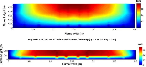
To ascertain whether the velocity profiles were correct the data of the six profiles were collated in a XYZ data file, where X and Y are the spatial coordinates giving the position of the point velocity V. The data was imported into MATLAB® where a velocity contour plot was created. This was integrated using a triangulation algorithm to establish the average velocity which was compared with the value measured by the magnetic flow meter in the flume loop. The contour plot of the 5.26% w/w CMC at Re = 164 is shown in Fig. 6. The difference between the flow rates measured by the flow meter and the integrated contour plot was 6.3%. For the 5.29% v/v bentonite suspension at Re = 438 shown in Fig. 7, the difference between the two values was 6.42%. This inspires confidence in the reliability of the detailed velocity measurements presented here. Tables 1 and 2 summarize the range of experimental conditions encompassed here. The undulations in the isobars are caused by the number of flow profiles that were available. If more data were available these lines would have been smoother.
Figure 6. CMC 5.26% experimental laminar flow map (Q = 6.79 l/s, ReH = 164).
Table 1. CMC 5.26% w/w fluid parameters and flow conditions.
Q (l/s)
H (mm)
θ
(deg) ReH
τy
(Pa) Regime K n
2.78 43.8 1 64 0 Lam 0.92 0.69
6.79 58.7 1 164 0 Lam 0.92 0.69
24.3 91.8 1 570 0 Trans 0.92 0.69 30.12 103 1 706 0 Trans 0.92 0.69
Table 2. Bentonite 5.29% w/w fluid parameters and flow conditions.
Q (l/s) H (mm)
θ
(deg) ReH
τy
(Pa) Regime K n
3.12 22.6 1 438 2.8 Lam 0.008 1
4.36 24.3 1 723 2.8 Lam 0.008 1
6.74 28 1 1276 2.8 Trans 0.008 1
14.165 39.3 1 2817 2.8 Turb 0.008 1
3.27 13.6 2 1151 2.8 Lam 0.008 1
Laminar sheet flow of a power law fluid
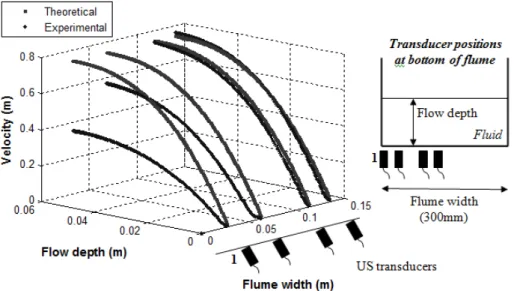
An example of a centreline plot for 5.26% w/w CMC at a flow rate of 2.78 l/s and at a flume slope of 1 degree is shown in Fig. 8. Also included here are the predictions of Eqs. (4) and (5). As can be seen there is a good correlation of the prediction with the experimental data. Figure 9 shows how the measured profile
deviates from the theoretical profile less than 100 mm away from the centre. Coussot (1994) suggested that in such a flume sheet flow can be assumed if the depth to width ratio is less than 1:10 (for a 300 mm wide flume the flow depth must be less than 30 mm to be sheet flow). The aspect ratio of the present flow is 1:2.5, which is much deeper than the 1:10 suggested by Coussot (1994).
0 0.005 0.01 0.015 0.02 0.025 0.03 0.035 0.04 0.045 0
0.05 0.1 0.15 0.2 0.25 0.3 0.35 0.4
Distance from transducer (m)
V
e
lo
c
it
y
(
m
/s
)
Theory Experimental
Figure 8. Sheet flow experimental versus theoretical at centreline for CMC 5.26% w/w at slope of 1 degree and flow rate of 2.78 l/s (laminar flow).
Figure 9. CMC 5.26% flume centre to wall experimental profiles vs. Eq. (6).
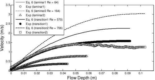
In Fig. 10, the progression of velocity profile measurements in laminar and transitional open channel flow is shown. It can be seen that the sheet flow profile only holds for the laminar flow conditions, as the assumption is also inherent in the derivation of Eqs. (4) and (5). The UVP measurements in transitional flow reach a maximum velocity (peak) and then decrease with increasing flow depth. This is due to the maximum measurable velocity and depth constraint in UVP systems. When using UVP a compromise between the maximum measurable velocity and the maximum measurable depth has to be made, but since this is not possible in
J. of the Braz. Soc. of Mech. Sci. & Eng. Copyright 2012 by ABCM July-September 2012, Vol. XXXIV, No. 3 / 281 0 0.01 0.02 0.03 0.04 0.05 0.06 0.07 0.08 0.09 0.1
0 0.5 1 1.5 2 2.5 3 3.5
Flow Depth (m)
V
e
lo
c
it
y
(
m
/s
)
Eq. 6 (laminar1 Re = 64) Exp (laminar1) Eq. 6 (laminar2 Re = 164) Exp (laminar2)
Eq. 6 (transition1 Re = 570) Exp (transition1) Eq. 6 (transition2 Re = 706) Exp (transition2)
Figure 10. CMC 5.26% flume centre profiles vs. Eq. (6) for laminar, transitional and turbulent.
Laminar sheet flow of a Bingham plastic fluid
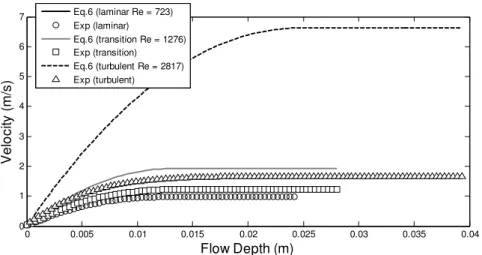
The centreline velocity profile showing the model predictions and the experimental data for the 5.29% v/v bentonite suspension for a flow rate of 3.27 l/s at a 2 degree slope is shown in Fig. 11. Again the agreement between the two seems to be good. However, the velocity gradients close to the flume surface (0 – 0.01 m) do not agree very well. This is due to the combination of the transducer installation method (see Fig. 4) and high velocity gradient of the Bingham profile. There is an increase in velocity at the surface interface due to influence of the cavity, which distorts the measured velocity profile. Note that this distortion did not occur during the CMC tests, which suggests that the cavities have a more significant influence on plug flows where the velocity gradients are high. It is also interesting to note that for the 5.29% w/w bentonite suspension the deviation of the predicted from the measured profile with distance from the centreline (see Fig. 12) is not so sudden as for CMC (see Fig. 9). This could be ascribed to the formation of the plug which extends towards the side wall. The sheet flow model still holds to about 20 mm from the side wall. The aspect ratio in this instance is 1:21, which is better than the 1:10 set as a limit for the sheet flow by Coussot (1994). In Fig. 13 the progression of velocity
from laminar to transition to turbulence is shown. It can be seen that the sheet flow profile only holds for the laminar flow similar to what was discussed for CMC.
0 0.002 0.004 0.006 0.008 0.01 0.012 0.014 0.016 0
0.2 0.4 0.6 0.8 1 1.2 1.4
Distance from transducer (m)
V
e
lo
c
ity
(
m
/s
)
Theory Experimental
Figure 11. Sheet flow experimental versus theoretical at centreline for bentonite 5.29% v/v at slope of 2 degrees and flow rate of 3.27 l/s (laminar flow).
0 0.005 0.01 0.015 0.02 0.025 0.03 0.035 0.04 0
1 2 3 4 5 6 7
Flow Depth (m)
V
e
lo
c
ity
(
m
/s
)
Eq.6 (laminar Re = 723) Exp (laminar)
Eq.6 (transition Re = 1276) Exp (transition) Eq.6 (turbulent Re = 2817) Exp (turbulent)
Figure 13. Bentonite 5.29% flume centre profiles vs. Eq. (6) for laminar transitional and turbulent flow.
Establishing in-line rheology using UVP and depth in flume
For open channel flow, it is possible just as for pipe flow to establish the rheological parameters by fitting the theoretical equation, in this case Eqs. (4) and (5) to the experimental data. Only one velocity profile measurement at the centre of the flume and the corresponding flow depth is required. By using a fitting procedure the rheological parameters τy, K and n can then be varied until the
error between the theoretical and the measured profile data is a minimum.
To test this conjecture, two fluids were used. The theoretically optimized and the experimental velocity profiles for 5.26% CMC are depicted in Fig. 14.
In Fig. 15, rheograms using the rheological parameters obtained from the flume are compared with those obtained from the tube viscometer. As can be seen, there is excellent agreement between the two flow curves. In Fig. 16 and Fig. 17, a bentonite suspension at 5.4% w/w concentration was used and similar results were obtained.
0 0.005 0.01 0.015 0.02 0.025 0.03 0.035 0.04 0.045
0 0.05 0.1 0.15 0.2 0.25 0.3 0.35 0.4
Distance from transducer (mm)
V
e
lo
c
it
y
(
m
/s
)
Theoretical Experimental
Figure 14. Sheet flow experimental vs. theoretical optimised fit for CMC 5.26%.
0 100 200 300 400 500 600 700 800 900 1000
0 20 40 60 80 100 120 140
Shear rate (s-1)
S
h
e
a
r
s
tr
e
s
s
(
P
a
) Pipe rheology
Sheet Flow Fit Pipe error 10%
Figure 15. Sheet flow vs. pipe flow rheology for CMC 5.26%.
0 0.005 0.01 0.015 0.02 0.025 0
0.1 0.2 0.3 0.4 0.5 0.6 0.7
Distance from transducer (mm)
V
e
lo
c
it
y
(
m
/s
)
Theoretical Experimental
J. of the Braz. Soc. of Mech. Sci. & Eng. Copyright 2012 by ABCM July-September 2012, Vol. XXXIV, No. 3 / 283
0 100 200 300 400 500 600 700 800 900 1000
2 4 6 8 10 12
Shear rate (s-1)
S
h
e
a
r
s
tr
e
s
s
(
P
a
) Pipe rheologySheet Flow Fit
Pipe error 10%
Figure 17. Sheet flow vs. pipe flow rheology for bentonite 5.29%.
Finally, it is appropriate to mention here that the model prediction is very sensitive to flow depth and yield stress, as can be seen in Fig. 18 and Fig. 19. When the value of the yield stress is changed from 2.8 to 2.6 Pa (8% change) the maximum velocity in the profile changes by 26%. This indicates that extreme care needs to be exercised in extracting the values of the rheological parameters from the velocity profiles. Also, it needs to be emphasized here that once the actual velocity profile is available, one can fit any suitable viscosity model simply by replacing Eqs. (4)-(6) by corresponding expressions for the model of choice.
0 0.005 0.01 0.015 0.02 0.025 0
0.2 0.4 0.6 0.8 1 1.2 1.4
Distance from transducer (m)
V
e
lo
c
ity
(
m
/s
)
Theory Experimental
Figure 18. Bentonite 5.29% sensitivity to yield stress 2.8 Pa.
0 0.005 0.01 0.015 0.02 0.025 0
0.2 0.4 0.6 0.8 1
Distance from transducer (m)
V
e
lo
c
ity
(
m
/s
)
Theory Experimental
Figure 19. Bentonite 5.29% sensitivity to yield stress 2.6 Pa.
Conclusions
The De Kee et al. (1990) model for predicting laminar sheet flow for pseudoplastic and yield pseudoplastic fluids has been validated with velocity profiles created by the non-invasive UVP method. As the tests were conducted in a 300 mm wide flume, the depth to which the sheet flow paradigm could be used was found to be 71.7 mm for CMC and 24.3 mm for bentonite, both in laminar flow at a one degree slope. Further tests are required in order to determine the exact limitations of the theoretical model for laminar sheet flow.
A new non-intrusive method for determining the rheology of a fluid flowing in a flume has been developed (UVP-FD). One velocity profile measured at the centreline with the UVP system and the flow depth is required. By fitting the model to the experimental data and optimizing the rheological parameters a good correlation with the in-line tube viscometer has been achieved. The advantage is that only one velocity profile is required instead of flow curves over a range of flow rates in at least 2 tubes. Complete velocity profiles over the whole flume cross-section were created using six profiles and it should be now possible to determine the wall shear stresses around the perimeter of the flume cross-section. Finally, it needs to be emphasized here that there are situations (like in food industry) where it is not possible to divert the flow into a bypass line (acting as a tube viscometer). On the other hand, UVP is used routinely as a tool to monitor the product quality and therefore, the scheme developed herein is a “non-invasive” tool to extract steady shear rheology of a fluid.
Acknowledgements
The financial support of this work from the National Research Foundation (NRF) and the Cape Peninsula University of Technology (CPUT) is acknowledged. We are also grateful to the constructive comments offered by the reviewers of this manuscript.
Nomenclature
A = area of flow, m2 D = pipe diameter, m
g = acceleration due to gravity, m/s2 h = depth of fluid in channel, m K = fluid consistency index, Pa.sn
L = pipe length, m
n = flow behavior index, dimensionless
n' = apparent flow behavior index, dimensionless Od = Oldroyd number, dimensionless
P = wetted perimeter, m Rh = hydraulic radius, m
Re = Reynolds number, dimensionless
ReH = Haldenwang Reynolds number, defined by Eq. (7),
dimensionless
V = average velocity, m/s <
z
V = velocity for
0
≤
x
≤
x
0,m/s >z
V
= velocity forx
0≤
x
≤
h
,m/s W = channel width, mX = vertical position in flume, m X0 = vertical position of plug interface, m
Greek Symbols
γ& = shear rate, s-1
α = angle of flume from the horizontal, degrees β = numerical constant in Oldroyd number formula ρ = fluid density, kg/m3
τxz = shear stress at any level in the fluid, Pa
τy = yield stress, Pa
References
Alderman, N.J. and Haldenwang, R., 2007,“A review of Newtonian and non-Newtonian flow in rectangular open channels”, Hydrotransport 17, The Southern African Institute of Mining and Metallurgy and the BHR Group, Cape Town, South Africa, pp. 87-106.
Astarita, G., Marucci, G. and Palumba, G., 1964, “Non-Newtonian flow along inclined plane surfaces”, I & EC Fundamentals, Vol. 4 No. 3, pp. 333-339.
Bergström, J. and Vomhoff, H., 2004, “Velocity measurements in a cylindrical hydrocyclone operated with an opaque fibre suspension”,
Minerals Engineering, Vol. 17, No. 5, pp. 599-604.
Birkhofer, B.H., 2007, “Ultrasonic In-Line Characterization of Suspensions”, Laboratory of Food Process Engineering, Institute of Food Science and Nutrition, Swiss Federal Institute of Technology (ETH), Zurich, Switzerland.
Bouillard, J., Alban, B., Jacques, P. and Xuereb, C., 2001, “Liquid flow velocity measurements in stirred tanks by ultra-sound Doppler velocimetry”,
Chemical Engineering Science, Vol. 56, pp. 747-754.
Cantelli, A., 2009, “Uniform Flow of Modified Bingham Fluids in
Narrow Cross Sections”, Journal of Hydraulic Engineering, Vol. 135, No. 8,
pp. 640-650.
Chhabra, R.P., 2006, “Bubbles, Drops and Particles in Non-Newtonian Fluids”, second edition, Boca Raton, CRC Press.
Chhabra, R.P & Richardson, J.F., 2008, “Non-Newtonian Flow and Applied Rheology”, IInd edition, Oxford, Butterworth-Heinemann.
Coussot, P., 1994, “Steady laminar flow of concentrated mud suspensions in open channels”, Journal of Hydraulic Research, Vol. 4, No. 32, pp. 535-558. De Kee, D., Chhabra, R.P., Powley, M.B. and Roy, S., 1990, “Flow of viscoplastic fluids on an inclined plane: evaluation of yield stress”, Chem. Eng. Comm., Vol. 96, pp. 229-239.
Ein-Mozaffari, F., and Upreti, S.R., 2009, “Using ultrasonic Doppler velocimetry and CFD modeling to investigate the mixing of non-Newtonian
fluids possessing yield stress”, Chemical Engineering Research and Design,
Vol. 87, pp. 515-523.
Fernandez, L. Gonzáles, A and Fuentes, R., 2010, “Flow of highly concentrated, extended particle size distribution slurries in open channels in laminar, transition and turbulent flow”, Hydrotransport 18: 18th International Conference on the Hydraulic Transport of Solids in Pipes, Rio de Janeiro, Brazil, pp. 167-182.
Franca, M.J. and Lemmin, U., 2006, “Eliminating velocity aliasing in
acoustic Doppler velocity profiler data”, Measurements in Science and
Technology, Vol. 17, pp. 313-322.
Fuentes, R., 2004, “Slurry flumes in Chile”, (Keynote Address). Hydrotransport 16: 16th International Conference on the Hydraulic Transport of Solids in Pipes, Santiago, Chile.
Haeri, S. and Hashemaabadi, S.H., 2009, “Experimental study of
gravity-driven film flow of non-Newtonian fluids”, Chem. Eng. Comm., Vol. 196, pp.
519-529.
Haldenwang, R., Slatter, P.T. and Chhabra, R.P., 2002,“Laminar and
transitional flow in open channels for non-Newtonian fluids”,
Hydrotransport 15: 15th International Conference on the Hydraulic Transport of Solids in Pipes, Banff, Canada, pp. 755-768.
Haldenwang, R., 2003, “Flow of non-Newtonian fluids in open channels”, Unpublished D.Tech thesis, Cape Technikon, Cape Town, South Africa.
Haldenwang, R. and Slatter, P.T., 2006, “Experimental procedure and
database for non-Newtonian open channel flow”, Journal of Hydraulic
Research, Vol. 44, No. 2, pp. 283-287.
Haldenwang, R., Slatter, P.T. and Chhabra, R.P., 2010, “An experimental study of non-Newtonian fluid flow in rectangular flumes in laminar, transition and turbulent flow regimes”, Journal of the South African Institution of Civil Engineering, Vol. 52, No. 1, pp. 11-19.
Huang, X. and Garcia, M.H., 1998, “A Herschel-Bulkley model for mud
flow down a slope”, Journal of Fluid Mechanics, Vol. 374, pp. 305-33.
Kotzé, R., Haldenwang, R. and Slatter, P.T., 2008, “Rheological characterisation of highly concentrated mineral suspensions using an ultrasonic velocity profiling with combined pressure difference method”,
Applied Rheology, Vol. 18, pp. 62114-62124.
Kotzé, R., Wiklund, J., Haldenwang, R. and Fester, V., 2011, “Measurement and analysis of flow behaviour in complex geometries using
the Ultrasonic Velocity Profiling (UVP) technique”, Flow Measurement and
Instrumentation,Vol. 22, pp. 110-119.
Kozicki, W. and Tiu, C., 1967, “Non-Newtonian flow through open channels”, Canadian Journal of Chemical Engineering, Vol. 45, pp. 127-134.
Kozicki, W. and Tiu, C., 1986, “Parametric modelling of flow
geometries in non-Newtonian flows”, In: Encyclopedia of Fluid Mechanics,
Vol. 7, pp. 199-252.
Kuttruff, H., 1991, “Ultrasonics: Fundamentals and Applications”, London and New York, Elsevier Applied Science.
Laba, D., 1993, “Rheological Properties of Cosmetics and Toiletries”, Marcel Dekker, Inc. New York.
Met-Flow SA., 2002, “UVP Monitor – Model UVP-DUO User’s Guide. Software version 3”, Met-Flow SA, Lausanne, Switzerland.
Müller, M., Brunn, P.O. and Wunderlich, T., 1997, “New Rheometric
Technique: the Gradient-Ultrasound Pulse Doppler Method”, Applied
Rheology, Vol. 7, pp. 204-210.
Ouriev, B., 2000, “Ultrasound Doppler Based In-Line Rheometry of Highly Concentrated Suspensions”, ETH dissertation No. 13523, ISBN 3-905609-11-8, Zurich, Switzerland.
Ouriev, B. and Windhab, E., 2003, “Novel ultrasound based time averaged flow mapping method for die entry visualization in flow of highly
concentrated shear-thinning and shear-thickening suspensions”,
Measurements in Science and Technology, Vol. 14, pp. 140-147.
Sad Chemloul, N., Chaib, K. and Mostefa, K., 2009, “Simultaneous Measurements of the Solid Particles Velocity and Concentration Profiles in Two Phase Flow by Pulsed Ultrasonic Doppler Velocimetry”, Journal of the Brazilian Society of Mechanical Sciences and Engineering, Vol. XXXl, No. 4, pp. 333-343.
Steger, R., 1994, “OptischUnd Akustische Metoden in Der Rheometrie”, Erlangen: University of Erlangen, pp. 1-100.
Takeda, Y., 1986, “Velocity Profile Measurement by Ultrasound Doppler Shift Method”, Int. J. Heat Fluid Flow, Vol. 7, No. 4, pp. 313-318.
Takeda, Y., 1995, “Velocity Profile Measurement by Ultrasonic Doppler
Method”, Experimental Thermal and Fluid Science, Vol. 10, pp. 444-453.
Takeda, Y., 1999, “Ultrasonic Doppler Method for Velocity Profile
Measurement in Fluid Dynamics and Fluid Engineering”, Experiments in
Fluids, Vol. 26, pp. 177-178.
Takeda, Y. and Kikura, H., 2002, “Flow mapping of the mercury flow”,
Experiments in Fluids, Vol. 32, pp. 161-169.
Wiklund, J., 2007, “Ultrasound Doppler Based In-Line Rheometry: Development, Validation and Application”, SIK – The Swedish Institute for Food and Biotechnology, Lund University, Sweden, ISBN 978-91-628-7025-6. Wiklund, J., Shahram, I. and Stading, M., 2007, “Methodology for in-line rheology by ultrasound Doppler velocity profiling and pressure difference techniques”, Chemical Engineering Science, Vol. 62, pp. 4159-4500.