A Discriminant Model of Network Anomaly Behavior Based on Fuzzy Temporal Inference

A Discriminant Model of Network Anomaly Behavior

Based on Fuzzy Temporal Inference

Ping He

Department of Information Liaoning police Academy

Dalian 116036, China

Abstract—The aim of this paper is to provide an active inference algorithm for anomalous behavior. As a main concept we introduce fuzzy temporal consistency covering set, and put forward a fuzzy temporal selection model based on temporal inference and covering technology. Fuzzy set is used to describe network anomaly behavior omen and character, as well as the relations between behavior omen and character. We set up a basic monitoring framework of anomalous behaviors by using causality inference of network behaviors, and then provide a recognition method of network anomaly behavior character based on hypothesis graph search. As shown in the example, the monitoring algorithm has certain reliability and operability.

Keywords- network anomaly behavior; anomalous omen; fuzzy temporal; set covering; hypothesis graph.

I. INTRODUCTION

Network anomaly behavior monitoring is a hotspot in reaches of network security. Up till now the basic idea of network anomaly discriminant lies in anomaly detection method, provided by Denning in 1987[1]. That is to say, according to abnormality situations of audit statement in monitoring system, the bad behaviors (i.e. events of violating safety norms) in network can be detected. The most study on network anomaly detection is based on the theory of data analysis. For example, probability and statistical method [2], data mining method [3], artificial immune algorithm [4], and corresponding artificial intelligence method [5] and so on. But the above methods have common constraint condition-data completeness.

To a certain extent, this condition is implementable. Meanwhile, a superior false alarm rate exists relatively. So it can not satisfy the requirement about reliability of network monitor. Literature [5] introduced an analysis method based on knowledge diagnosis. Literature [6] put forward a method for anomaly detection based on direct inference. Literature [7] brought forward an extrapolation inference diagnosis model based on set covering (GSC). It is one of knowledge diagnosis models with many advantages, such as intuition, parallel, leading into heuristic algorithm easily. Probability causality was led into the model by Peng in literature [7，8].

In order to solve problems about anomaly detection for fuzzy network behavior, literature [9] combined intrusion detection model with fuzzy theory. Among the above mentioned methods, it had no consideration of causality

between anomalous behaviors and data in network, as well as temporal constraint relationship with each other. Because data features come into being with network anomaly behaviors, the interaction discriminant method based on anomalous behavior-data is an active network monitor and defensive strategy.

In this paper, we propose a fuzzy temporal inference method, and describe inaccuracy for network temporal knowledge by using of fuzzy set, and then constitute a model of network temporal generalized behaviors covering (NTGSBC). Finally, discriminant results are satisfactory.

II. NETWORK TEMPORAL GENERALIZED BEHAVIORS

COVERING (NTGSBC)

A. Fuzzy Temporal of Network Behaviors

Fuzzy temporal analysis method has reached satisfied result in the research of fault diagnosis [3, 4]. In this section, we will set up an inference method for network anomaly behavior by using the analysis method in literature [4]. As we know, the main character of complexity in network behaviors is time fuzziness of its behavior state. In fact, occurring temporal of network behavior is an uncertain time based on interval transition.

It is a fuzzy period of time, so definition is as follows:

Definition 2.1 [4]. Network behavior happened in a network fuzzy time interval (N.F.T.I), supposeIbe a trapezoid fuzzy number (T.F.N) defined on the network behavior time axis T，

I



( , , ,



_t

t t

_{s f}



_h

)

, the membership degree



_I

( )

t

is as follows

0,

(

) /

,

( )

1,

(

) /

,

0,

s l

s l l s l s

I s f

f h h f f h

f h

t

t

t

t

t

t

t

t

t

t

t

t

t

t

t

t

t

t





















_

_



 



 







_

 



_

_

_{ }

_





_

_



(1)

( )

0,

(

) /

,

1,

0,

s l

s l l s l s

start I

s

s

t

t

t

t

t

t

t

t

t

t

t











 



  



 



 

_





_



(2)

The end time in

I

is expressed by end (

I

), and it is defined as:

( )

0,

1,

(

) /

,

0,

f

f end I

f h h f f h

f h

t

t

t

t

t

t

t

t

t

t

t

















_



 

_

_

_{ }

_





_

_



(3)

When

t

_s



t

_f



t

,Ican be reduced to a network fuzzy time point(F.T.P),

I



( , , ,



_l

t t



_h

)

, so it turns into a triangular fuzzy numbers(T.F.N). When

 

_l



_h



0

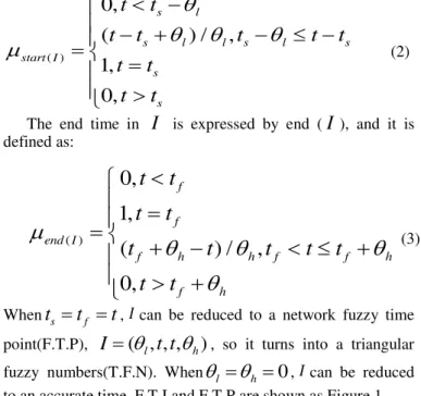
,Ican be reduced to an accurate time. F.T.I and F.T.P are shown as Figure 1.

Figure 1. F.T.I and F.T.P

Fuzzy difference between two (T.F.N) reflect a kind of fuzzy temporal in the real network, and it exits

1

  

(1) (2) (1) (2) (1) (2) (1) (2)

2

(

l

,

s

,

f f

,

f s

,

h l

)

I





t

t



t

t



t







4

B. Detection model for Anomalous Behavior

Definition 2.2 A discriminant model of network anomaly behavior is a relation mapping inversion space of data – behavior with fuzzy temporal, the formal representation can be shown as

P



A D R DEL D DOCT

, , ,

,



,



, where

(1)

A



{ ,

a a

_{1 2}

,...,

a

m

}

, it is a non-empty finite set with

anomalous behavior;

(2)

D



{

D D

₁

,

₂

,...,

D

n

}

, it is a non-empty finite set with

anomalous data;

(3)

R

 

A D

is a relationship of network anomaly behavior defined on

A D



.



a D

i

,

j



R

, if and only if

behavior

a

_i reflects data

D

_j in network, and

 

D

_j

D

,

there exists an element

a

_i



A

at least, such that

,

i j

a D

R





;

(4)DEL is a delay matrix on

|

A

| |



D

|

. For ( , ) ( , )

,

,

d i j i j d

i j l h

a D

R DEL









i , j

=(

, a

, A

,

)

is a

F.T.I. It expresses the delay time approximately “from ( , )i j

a

to

A

( , )i j ” between “the beginning of anomalous behavior” and

“the beginning of data

D

j ”; for



a D

i

,

j



R

，

DEL

i , j

has no definition.

(5)

D





D

expresses a known anomalous data set of the discriminent target P. DOCT expresses |D| dimensional vector.

For

D

_j



D

, DOCT

( )

j



(



_lm

,

t

_s( )j

,

t

( )_fj

,



_hm

)

is a F.T.I. It expresses the appearance time of the known anomalous data

j

D

approximately “from

t

( )_Dj to

t

( )_Dj ”. For

,

( )

j

D



D DOCT j

 has no definition.

(

_j

)

{

_i

|

_i

,

_i

,

_j

}

cause D



a a

 

A

a D



R

is an all

possible anomalous behavior set caused

D

_j.

cause D

(



)



(

)

j

j

D D

cause D





U

is an all possible anomalous data set

caused

D

.

( )

i

{

j

|

j

,

i

,

j

}

effect a



D

D



D



a D



R

is a data

set caused by anomalous behavior

a

_i .

effect A

(

I

)



( )

i I

i a A

effect a



U

is an all possible data set caused by

I

A



A

. For

A

I

A D

,

D

,







D

Iis a covering of

D

 ,

if and only if

D





effect A

(

_I

)

. Network anomaly behavior

a

_i



A

is relative to the known anomalous data

j

D



D

 , the start time of anomalous behavior

(

)

i j

a



cause D

is as follows:

begin OCT a D



(

_i

|

_j

)



begin DOCT j

(

(

( , )

DEL i j

5

The end time of anomalous behavior

a

i, relative to

D

j, is

as follows:

(

i

|

j

)

(

( ))

end



OCT a D



end DOCT j

(6)

Definition 2.3 For

,

( )i

i

a



A D





D

 ，

{ }

a

_i is a temporal consistency covering on

D

( )i , if

(2)

min(max

_begin

(

_i

|

( )i

)( ), max

_end

( |

_i ( )i

)( ))

i T i T

a D

t

a D

t











 



(7)

( )

~ ( )

(

|

)

(

|

)

i j

i

i i j

s S

begin a D

begin OCT a D

 





_I



(8)

( )

~ ( )

(

|

)

(

|

)

i j

i

i i j

D D

end a S

end

OCT a D

 





_I



(9)

0

 



1

is athreshold constant with temporal consistency, ~

I

expresses intersection of fuzzy sets.

Different from literature [1,4], the solution of discriminant target in NTGSBC is not only pointed out anomalous behavior set

A

I covered consistency data set

D



, but also ensured

D

_j



D

 caused by

a

_i



A

_I , because of temporal consistency requirements.

Definition 2.4 Suppose a complete explanation of discriminant target P in network behaviors be

exp( ) {( ,

_i

( )) |

_{i i}

,

Co



P



a D a



a



A

D d



( )

_i



D



}

,

and satisfying the following conditions:

(1) For

( ,

a D a

i

( ))

i

Co

exp( )

P



_

_

_，

{ }

a

i is a

temporal consistency covering on

D a



( )

_i .

(2) ₁

( , ( )) exp( )

( )

i i

i

a D a Pa P

D a

D



 

 



U

expresses a known

anomalous omen set.

{ | (( ,

( ))

exp( )}

I i i i

A



a

a D a





Co



P

is called an

explanation omen set of complete explaining

Co



exp( )

P

. Obviously

A

_Icovers

D

.

Definition 2.5 Suppose a partial explanation of discriminant target P in network behaviors be

exp( ) {( ,

i

( )) |

i i

,

( )

i

}

Pa



P



a D a



a



A D a





D

 , and satisfying the following conditions:

(1) For

( ,

a D a

i

( ))

i

Pa

exp( )

P



_{ }

_，

{ }

a

i is a temporal

consistency covering on

D a



( )

_i . (2) ₁

( , ( )) exp( )

( )

i i

i

a D a Pa P

D

M

a

D



  

 



_U



,

and for

D

D

1

,



_



2

(

)

I

{ | ( ,

i i

( ))

i

exp( )}

cause D





A



a

a S



a



Pa



P

.

2

D

 is called a non-covering anomaly data set of

exp( )

Pa



P

,

A

_I is called an explanation anomaly behavior set of

Pa



exp( )

P

.

In the definition 2.5, due to

cause(

D

₂

)



A

_I, it has

2

(

I

)

D





effect A

, namely

A

_I is a covering of

D

₂, so

I

A

is a covering of the whole known anomalous data set

1 2

D





D





D

. But there exists a constraint condition of

temporal consistency, all the

a

_iin

A

_Ionly can explain (or

cover)

D

₁, a part of

D

.

A complete solution

Co



exp( )

P

of discriminant target P is a complete explanation of P. and the cardinality of anomalous data set

D

_I , explained

Co



exp( )

P

, is minimum. A partial solution of P is a partial explanation

exp( )

Pa



P

, and the cardinality of non-covering anomaly

omen set

D

₂ is minimum.

III. SOLVING DISCRIMINANT TARGET IN NETWORK BEHAVIORS

A. Hypothesis Graph

Solving problems of a discriminant target in network behaviors is based on a search method of hypothesis graph. Hypothesis graph is defined by network nodes and successor.

Definition 3.1Suppose a node

n

_i be ( ) ( ) ( )

1 2

(

i

,

i

,

i

)

i I

n



A

D



D

 ,

in the hypothesis graph G(P) of discriminant target P, where

( ) ( ) ( )

1

( ) ( )

2 1

,

(

),

i i i

I I

i i

A

A D

D

effect A

D

D

D

 

  









I

.

( ) ( ) ( )

1 2

(

i

,

i

,

i

)

i I

n



A

D



D



in G(P) is divided into three types:

1) Complete end node: for

n D

_i

,

₂( )i





。

2) Partial end node:

n D

_i

,

₂( )i





and

( ) ( ) 2

(

i

)

i

I

cause D





A

.

3) Non-end node: the other nodes except the above two types nodes.

Definition 3.2 For the node

(

( )k

,

₁( )k

,

₂( )k

)

k I

n



A

D



D

 in

the hypothesis graph G(P), if it has

D

_j



D

₂( )k

,

d

_i



cause

( )

(

D

_j

)



A

_Ik , then asuccessornode of

n

_kis as follows:

( ) ( ) ( )

1 2

( ) ( )

2 2

(

,

)

(

{ },

(

( )),

(

( )))

k k k

k i I i

k k

i i

succ n a

A

a

D

some D

effect a

D

some D

effect a

 

 





U

U

I

I

Where

{ }

a

_i is a temporal consistency covering on

( ) ( )

2 2

(

k

( ))

k

( )

i i

some D



I

effect a



D



I

effect a

.

When constructed G (P), it began from an initial node

0

( , ,

)

generated its successor node, until to the expansion node translated into non-expansion complete nodes or partial nodes. The following two theorems point out corresponding relationship in G (P) between a path and discriminant targets.

Theorem 3.1 Suppose a path in hypothesis graph G (P), from an initial node

n

₀



( , ,

 

D



)

to some complete end node

n

l



(

A

I( )l

,

( ) ( )

1

,

2

)

l l

D



D

 , be (without loss of generality)

0

, ,..., ,

1 i i1

,..., ,

l

n n

n n

_

n

where

n

_i1is a successornode of

n

_i, ( ) ( ) ( )

1 2

0

1,

(

i

,

i

,

i

),

i I

i l

n

A

D



D



  



then

( 1) ( ) ( 1) ( )

1 1

( )) |

_{k k I}i _Ii

,

( )

_k i i

,

D a



a



A





A

D a





D

 



D



0

  

i l

1}

is a complete explanation

Co



exp( )

P

of the target P, and the set of anomalous behavior explanation

Co



exp( )

P

is

( )l

I I

A



A

.

Theorem 3.2 Suppose a path in hypothesis graph G(P),

from an initial node

n

₀



( , ,

 

D



)

to some partial end node

n

_l



(

A

_I( )l

,

D

₁( )l

,

D

₂( )l

)

, be (without loss of generality)

0

, ,..., ,

1 i i1

,..., ,

l

n n

n n

_

n

where

n

_i1is a successornode of

n

_i, ( ) ( ) ( )

1 2

0

  

i

l

1,

n

_i



(

A

_Ii

,

D

i

,

D

i

),

then

( 1) ( )

( 1) ( )

1 1

{

( )) |

,

( )

, 0

1}

i i

k k I I k

i i

S a

a

A

A

D a

D

D

i l

  

  









  

is a partial explanation

Pa



exp( )

P

of the target P, and the set of non-covering anomaly omen

Pa



exp( )

P

is

( )

2 2

l

D





D

 .

The proof of above two theorems is shown in appendix.

B. Operating process of the discriminant system

According to theorem 3.1and 3.2, the operating of monitor system is based on the search of hypothesis graph. If it exists complete end nodes in the final hypothesis graph G(P), then the complete explanation

Co



exp( )

P

of the target P can be obtained. And then a minimum in

|

A

_I

|

is taken for a complete solution

Co



exp( )

P

of the target P , where

A

_I is a set of explanation anomaly behavior

Co



exp( )

P

. If it only exits partial end nodes in G(P), then the partial explanation

Pa



exp( )

P

of the target P can be obtained. And then a minimum in

|

S

₂

|

is taken for a partial solution

exp( )

Pa



P

of the target P, where

S

₂ is a set of non-covering anomaly omen

Pa



exp( )

P

.

Solution procedure is as follows:

(1) Algorithm Solve-TGSC(A, D, R, DEL,

D

, MOCT)

(2) Variable

n

_i: node,

D

_j: data ,

a

_k: anomalous behavior, table OPEN, table CLOSE

(3)Begin OPEN: =

{

n

₀



( , ,

 

D



)}

(4) CLOSE: =



: {Initializing table OPEN, CLOSE} (5) While there are non-terminal nodes in OPEN do (6) Begin

n

_i: = POP(OPEN)

{Removing non-end node

n

_i



(

A

_I( )i

,

D

₁( )i

,

D

₂( )i

)

from table OPEN, and add to table CLOSE}

(7)

D

_j

:



select D

(

₂( )i

);

{Selecting

D

_jfrom

D

₂( )i } (8) For each

a

_k



cause s

( )

_j



A

_I( )i do

(9) Begin SUB: = choose

(

D

₂( )i

I

effect a

(

_k

))

{Constructing set SUB}

(10) For each

sub

_i



SUB

do (11) Begin such

n a

i

,

k =

( ) ( ) ( )

1 2

(

i

{ },

i

,

i

);

I k i i

A

U

a

D



U

sub D





sub

{Constituting successornode of

n

_i}

(12) INSERT such

n d

i

,

k ，OPEN ;{ renewing table

OPEN}

(13) End for End for End for

(14) If there are complete terminal nodes in OPEN

(15) Then solving the complete solution of problem P, return

C

o



sol P S

( ) ;

{theorem 3.1}

(16) Else solving the partial solution of problem P, return

( ) ;

Pa sol P S



{theorem 3.2} (17) End.

In the step (9), it constructs a set by using function choose, satisfying the following conditions

( ) 2

{

_i

|

_i i

SUB



sub sub



D



I

effect a

(

_k

),

sub

_i





}

(a) For

sub

i



SUB a

,{ }

k is a temporal consistency

covering.

(b) For

sub

_i



SUB

, It does not exist ( )

2

(

)

i

i k

sub



D



I

effect a

,

such that

sub

_j



sub

_i, and

{ }

d

_k is a temporal consistency covering on

sub

_i.

In the step (12), for successornode of

n

_i, ( ) ( ) ( )

1 2

( ,

)

(

j

,

j

,

j

)

j i k I

n



succ n a



A

D



D

 ， INSERT revises table OPENas follows:

(i) If

n

_jis a complete or partial end node,

n

_jwill be put

into the table OPEN directly. Otherwise

n

jis a non-end node,

(ii) If it has

n

_t



(

A

_I( )t

,

D

₁( )t

,

D

₂( )t

)

in the table OPEN and CLOSE, such that

D

₂( )j



D

₂( )t ,

A

_I( )t



A

_I( )j , then the node

n

_jis abandoned, the table OPEN is not change.

(iii) If it has

n

_t



(

A

_I( )t

,

D

₁( )t

,

D

₂( )t

)

in the table OPEN, such that

D

₂( )j



D

₂( )t ,

A

_I( )t



A

_I( )j , then the node

n

_tis deleted from the table OPEN, and put into the table CLOSE, meanwhile

n

_jis put into the table OPEN.

(iv) Otherwise,

n

_jis put into the table OPEN.

In afore-mentioned algorithm, the table OPEN is using to deposit expanding nodes, and the table CLOSE is using to deposit expanded nodes. In the process of constructing G(P), successornodes is generated in basis of causality and temporal constraint(temporal consistency) between anomalous behavior and anomalous omen. Suppose the graph is acyclic graph, and the number of nodes is limited. The complete or partial nodes can be obtained through successor expanded

succ n a

( , )

_{i k} after undergoing limited steps (no more than |D|). Therefore termination of algorithm is quite obvious.

IV. INSTANCE ANALYSIS

A discriminant target of network behaviors

, , ,

,

,

P



A D R DEL D DOCT





has the following definition :

1 2 3 4 5

{

,

,

,

,

}

D





D D D D D

,

A



{ ,

a a a

_{1 2}

,

₃

}

, then the relation matrix of behavior-data in network is as follows :

1

a

a

₂

a

₃

1 2 3 4 5

1 1

1

1 1

1 1

1 1

D D

R D

D D

 

 

 

 



 

 

 

 

Based on the theorem 3.1 and 3.2, it can be obtained the following values:

DOCT(1)=(1,8,10,1), DOCT(2)=(1,9.8,9.8,1), DOCT(3)=(1,12,13,1),DOCT(5)=(1,10,11,1)

(1,1)

(1, 3, 4,1),

(1, 3)

(1, 3, 3,1),

(2, 4)

(1, 7, 7,1),

(3,1)

(1,8,8,1),

DEL

DEL

DEL

DEL









(1, 2)

(1, 4.6, 5.7,1),

(2, 3)

(1, 4, 5,1),

(2, 5)

(1, 5, 6,1),

(3, 4)

(1, 9,10,1)

DEL

DEL

DEL

DEL









( 3 , 5 )

( 1, 6 ,

D E L



It takes a temporal consistency threshold



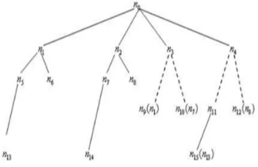
=0.6, it is taken the first in first out strategy the table OPEN, and generated a hypothesis graph, it is shown as Figure 2.

Figure 2. Hypothesis graph of discriminant target P

Where

0 1 1 1 2

2 1 3 3 3 1

( , ,

),

({ },{ ,

}),

({ },{

}),

({ },{ }),

n

D

n

a

D D

n

a

D

n

a

D

 











4 3 5 5 1 2 1 2 3

6 1 2 1 2 5 7 1 3 3 1

({ },{

}),

({ , },{ ,

,

}),

({ , },{ ,

,

}),

({ , },{

,

}),

n

a

D

n

a a

D D D

n

a a

D D D

n

a a

D D









8 1 3 3 5 9 3 1 1 2

10 3 1 1 3 11 3 1 5 1 2

({ , },{

,

}),

({ , },{

,

}),

({ , },{

,

}),

({ , },{

,

,

}),

n

a a

D D

n

a a

D D

n

a a

D D

n

a a

D D D









1 2 3 1 5 3 1 3 1 2

1 2 3 5

1 4 1 3 2 3 1 5

1 5 1 3 2 5 1 2 3

( {

,

} , {

,

} ) ,

( {

,

{

,

,

,

} ) ,

( {

,

,

} , {

,

,

} ) ,

( {

,

,

} {

,

,

,

} )

n

a a

D D

n

a a

a

D D

D D

n

a a a

D D D

n

a a a

D D D

D









Because of

D

₁( )i

U

D

₂( )i



D

 ，

n

_i is written

n

_i = ( ) ( )

1

(

i

,

i

)

I

A

D

 for short. In the beginning of algorithm, it is

taken

D

₁



D

₂(0)



D

 from a initial node

0

( , ,

)

n



 

D

 , then

a a

₁

,

₃



cause D

(

₁

)



A

_I(0). Based

on a behavior

a

₁ , it can construct sub-set

1 2 3

{{

,

},{

}}

SUB



D D

D

, and generate successor nodes

1

,

2

n n

in the basis of

n

₀, then put it into table OPEN. In the same way, based on

a

₃ , it can construct sub-set

1 3

{{

},{

}},

SUB



D

D

and then obtain the successor nodes

3

,

4

n n

in the basis of

n

₀.

( )

Co sol P





{( ,{

a

₁

D D

₁

,

₂

}), ( ,{

a

₂

D

₃

}), ( ,{

a

₃

D

₅

})}

. Partial end nodes

n

₆and

n

₁₄are corresponding to partial

solutions respectively. For example

n

₆ corresponds to

1 1 2 2 5

( )

{( ,{

,

}), ( ,{

})}

Pa



sol P



a

D D

a

D

, it is known

that the omen

m

₃does not explain. The occurrence time of each known omen and corresponding anomalous behavior is shown in Figure1.

V. CONCLUSION

The solution for network anomaly detection in this paper is a further development based on literature [5，6]. Actually, it is breadth- first search method. So the search cost is still greater, especially for a large amount of data, though the method presented in this paper makes pruning, in order to decrease the number of network nodes, by using of temporal consistency in the step of SUB, INSERT etc. Trying to resolve this conflict, a possible method is to convert the original method into depth-first search method by introducing node evaluation function, such as literature [7，8，9]. But in the model of NTGSBC, node evaluation function must reflect causality and temporal constraint between anomalous behavior and data at the same time. It is more complex than pure probability causality in literature [2, 3]. It is yet to be further studied about how to seek appropriate node evaluation function in the model of NTGSBC. The other possible solution is problem decomposition. For example, in total behavior detection system modeling of a large website, we will divide the total detection process into many subsystems according to structure and function of website system. And define the causality among subsystems. Moreover the subsystem itself is defined by the model of NTGSBC. Anomaly behavior detection process is separated into inner inference for NTGSBC monitor system and anomaly causality diffusion among subsystems. The advantage of this method is as follows: (1) the detection scale of subsystems, obtained after decomposition, is smaller. It is fit for NTGSBC modeling and problem solving. (2) Through problem decomposition and defining the diffusion causality among subsystems, multi-layered causality model about total monitor targets will be built up, based on two layer causality from anomalous behavior to data. Multi-layered causality model is more suitable for detection target describing and problem solving.

Temporal consistency set covering is defined in this paper. And based on this definition, we described the basic framework of NTGSBC and the method of problem solving. Fuzzy temporal information is introduced in the model of NTGSBC, it makes generalized inference detection model and method more fitting for practical problems in other fields. Certainly, more detailed studies should be continued in the further.

REFERENCES

[1] Bykova M, Ostermann S, Tjaden B. Detecting network intrusions via a statistical analysis of network packet characteristics. In: Proc. of the 33rd Southeastern Symp. on System Theory. 2001. 309314. http://masaka.cs.ohiou.edu/papers/ssst2001.pdf

[2] Denning DE. An intrusion-detection model. IEEE Trans. on Software

Engineering, 1987,13(2):222-232.

[3] Lee W, Stolfo SJ. A framework for constructing features and models for intrusion detection systems. ACM Trans. on Information and System Security, 2000,3(4):227-261.

[4] Valdes A, Skinner K. Adaptive, model-based monitoring for cyber attack detection. In: Debar H, M¨ L, Wu SF, eds. Proc. of the 3rd

Int!ˉlWorkshop on the Recent Advances in Intrusion Detection (RAID

2000). LNCS 1907, Heidelberg: Springer-Verlag, 2000. 80-93. [5] Aickelin U, Greensmith J, Twycross J. Immune system approaches to

intrusion detectionA review. In: Nicosia G, et al., eds. Proc. of the 3rd

Int!ˉl onf. on Artificial Immune Systems. LNCS 3239, Heidelberg:

Springer-Verlag, 2004. 316-329.

[6] Lee W, Stolfo SJ. A Data mining framework for building intrusion detection models. In: Gong L, Reiter MK, eds. Proc. of the !99 IEEE Symp. on Security and Privacy. Oakland: IEEE Computer Society Press, 1999. 120-132.

[7] Eskin E, Arnold A, Prerau M, Portnoy L, Stolfo SJ. A geometric framework for unsupervised anomaly detection: detecting intrusions in unlabeled data. In: Barbar¨ D, Jajodia S, eds. Applications of Data Mining in Computer Security. Boston: Kluwer Academic Publishers, 2002. 78-99.

[8] Proedru K, Nouretdinov I, Vovk V, Gammerman A. Transductive confidence machine for pattern recognition. In: Elomaa T, et al., eds. Proc. of the 13th European Conf. on Machine Learning. LNAI 2430, Heidelberg: Springer-Verlag, 2002. 381-390.

[9] Barbar¨ D, Domeniconi C, Rogers JP. Detecting outliers using transduction and statistical testing. In: Ungar L, Craven M, Gunopulos D, Eliassi-Rad T, eds. Proc. of the 12th ACM SIGKDD

Int!ˉl onf. on Knowledge Discovery and Data Mining. New York: ACM

Press, 2006. 55-64.

[10] Angiulli F, Pizzuti C. Outlier mining in large high-dimensional data sets. IEEE Trans. on Knowledge and Data Engineering, 2005, 17(2):203-215.

[11] Ghosh AK, Schwartzbard A. A study in using neural networks for anomaly and misuse detection. In: Proc. of the 8th USENIX Security Symp. 1999. 141-151.

http://www.usenix.org/events/sec99/full_papers/ghosh/ghosh.ps [12] Manikopoulos C, Papavassiliou S. Network intrusion and fault

detection: A statistical anomaly approach. IEEE Communications Magazine, 2002,40(10):76-82.

[13] Laskov P, Schafer C, Kotenko I. Intrusion detection in unlabeled data with quarter-sphere support vector machines. In: Proc. of the Detection of Intrusions and Malware & Vulnerability Assessment (DIMVA 2004). 2004. 71-82.

http://www2.informatik.hu-berlin. de/wm/journalclub/dimva2004.pdf AUTHORS PROFILE

He Ping is a professor of the Department of Information at Liaoning Police Academy, P.R. China. He is currently Deputy Chairman of the Centre of Information Development at Management Science Academy of China. In 1986 He advance system non-optimum analysis and founded research institute. He has researched analysis of information system for more than 20 years. Since 1990 his work is optimization research on management information system. He has published more than 200 papers and ten books, and is editor of several scientific journals. In 1992 awards Prize for the Outstanding Contribution Recipients of Special Government Allowances P. R. China.

APPENDIX

The proof of theorem 3.1is as follows: (1) Note

1

( 1) ( )

1 1

{( ,

( )) |

,

( )

, 0

1}

i i

k k k I l k

i i

Co

ps

a D a

a

A

A D a

D

D

i

l

  

  













  

,

as

n

_i1is a successornode of

n

_i, according to the definition

1

( ) ( ) ( ) ( )

1 2 2

( ) 2

( , )

( { }, ( ( )),

( ( ))),

i i k

i i i i

I k k

i

k

n succ n a

A a D some D effect a D

some D effect a

       

U U I

I

k

a

is a temporal consistency covering on

( ) ( )

2 2

(

i

(

_k

))

i

(

_k

)

some D



I

effect a



D



I

effect a

.

Due to

a

_k



cause D

(

_j

)



A

_I( )i ，it exists ( ) ( 1) ( ) ( ) ( )

{ }

a

_k

I

A

_Ii





,

A

_Ii



A

_Ii



A

_Ii

U

{ }

a

_k



A

_Ii



{ },

a

_k ( 1 ) (

.

i i

k I I

a



A





A

Based on

D

₂( )i



D





D

₁( )i , it exists

( ) ( ) ( ) ( )

1 2

,

1

(

2

(

))

,

i i i i

k

D



I

D







D



I

some D



I

effect a





Then it obtains

( 1) ( )

1 1

( ) ( ) ( )

1 2 1

( ) 2 ( ) ( ( )) ( ( )) i i k

i i i

k

i

k

D a D D

D some D effect a D some D effect a

             U I I

So for

(

a D a

_k

,



(

_k

))



Co



ps a

,{ }

_k



A

_Ii1



A

_li is a temporal consistency covering on

D a



(

_k

)

.

(2) In order to express itself clearly note

1 ( 1) ( ) ( 1) 1 ( 1) ( )

1 1

,

(

)

i i i i i i i

k I I k

a





A





A

D

 

a





D

 



D

 , then

( 1) ( 1)

0 1 ( , ( ))

(

)

(

)

k k i i k k i l a D a co ps

D a

D

a



    

    



U

U

A.1 A

proof by mathematical induction is adopted firstly. For

1

p

 

l

, the following expression holds

( 1) ( 1) ( 1)

1 0

(

)

i i p

k i p

D

 

a

 

D

   



U

A.2

When p=0, noticed that

S

₁(0)





for initial node

n

₀, it exits ( 1) ( 1) (1) (1)

0 0

(1) (0) (0 1)

1 1 1

(

)

(

)

i i

k k

i

D

a

D

a

D

D

D

         









U

.

Suppose the expression (A.2) is set up when

,

2

p



t t

 

l

, then ( 1) ( 1)

0 1

(

)

i i

k i t

D

 

a



  

U

( 1) ( 1) ( 2) ( 2)

0

( 1) ( 2) ( 1)

1 1 1

( 1) ( 1) 2

1 2 ( 2) 1

(

(

))

(

)

(

(

))

(

(

))

i i t t

k k

i t

t t t

t t t

k

t

D

a

D

a

D

D

D

D

some D

effect a

D

                    











U

U

U

I

U

So the expression (A.2) is set up. As well as ( ) ( ) ( )

1 2

(

l

,

l

,

l

)

l I

n



A

D



D

 is a complete end node,

( ) ( ) 1

,

2

l l

D





D D

 





, hence ( 1) ( 1) ( )

1 0 1

(

)

i i l

k i l

D

 

a



D



D



  





U

.

According to the results of expression (1) and (2), and definition 2.4, the set Co-ps is a complete explanation Co-exp

P for the problem P.

(3) As Co-ps is a Co-exp P of the problem P, according to definition 2.4, a fault set is as follows:

( 1)

0 1

( 1) ( 1) ( )

0 1

{

| ( ,

(

))

}

{

}

(

)

)

I k k k

i k i l

i i i

I I I

i l

A

a

a S a

Co

ps

a

A

A

A

         













U

U

.

Resembling the proof of the expression (A.2) in the step (2), a proof by mathematical induction is adopted. So the set of anomalous behavior explanation

Co



exp( )

P

is as follow:

( 1) ( ) ( )

0 1

(

i

)

i

)

i

I I I I

i l

A

A



A

A

  



_U





Theorem 3.2 is proved as follows: ( 1) {( _k, ( _k)) _k ( _Ii _Ii),

Paps a D a a  A  A

( 1) ( )

1 1

( ) i i, 0 1}

k

D a D  D   i l

(1) it is similar to the step (1) in theorem 3.1, it exists (a D ak, ( k)) Pa ps

 _{ }

.

{

a

k

}

is a temporal consistency

covering of D a( k)



.

(2) For the set Pa-ps, resembling the proof of step (2) in theorem 3.1, it can be obtained

( 1) ( 1) ( )

1

0 1

( , ( ))

( ) ( )

k k

i i i

k k i

i l

a S a Pa ps

D D a D a D



      

    



_U



_U

 B.1

Resembling the proof of step (3) in theorem 3.1, for Pa-ps, it exists

( 1)

0 1

{ ( , ( )) } { i }

I k k k k

i l

A a a D a Pa ps a 

  

   

_U

(B.2)



1 0 ) 1 (

)

(

   

_

_



l i i I i I i

I

A

A

A

As ( ) ( )

1

( i, i, i)

t I I

n  A D D is partial end nodes, so

Cause ( ) ( ) ( ) ( )

2 2 1 2

{ i i, i , i i

I

D A D  D DD D

Then combining with the expression (B.1) and (B.2), it exists ( ) 1 ( , ( )

(

)

k k l k I

a M a Pa po

D

D a

D

D



   

 



_U





.

For

( ) ( )

2 1 1 2

( ) 2 2

,

(

)

(

)

,

l l l I I

D

D

D

D

D

D

cause D

cause D

A

A

       

















2

(

)

{

| (

,

(

)

}.

I

k k k

cause D k

A

a

a D a

Pa

ps











