Outlier detection for improved clustering : empirical research for unsupervised data mining

i

OUTLIER DETECTION FOR IMPROVED

CLUSTERING

Jacob Hastrup Madsen (M2016087)

Empirical research for unsupervised data mining

Dissertation for obtaining the Master’s degree in Information

Management with a Specialization in Business Intelligence

and Knowledge Management

i

LOMBADA MEGI

LOMBADA MGI

Outlier Detection for Improved Clustering

Empirical Research for Unsupervised Data Mining Jacob Hastrup Madsen

MEGI

20

17

20

iii

NOVA Information Management School

Instituto Superior de Estatística e Gestão de Informação

Universidade Nova de Lisboa

OUTLIER DETECTION FOR IMPROVED CLUSTERING

by

Jacob H. Madsen

Dissertation proposal presented as partial requirement for obtaining the Master’s degree in Information Management with a Specialization in Business Intelligence and Knowledge Management

Advisor: Prof. Dr. Ana Cristina Costa

iv

ACKNOWLEDGEMENTS

To fellow students Jan Benedikt and Marcel Motta. Thanks for the good times of intensive studying during exam and project periods. A special thanks to Jan for always being supportive for whatever math or computational problem that would occour. One year in Lisbon is a year you will never forget.

To the Danish and European taxpayers, thank you for providing financial support and enabling me to go to Portugal and going on Erasmus semester in Germany.

v

ABSTRACT

Many clustering algorithms are sensitive to noise disturbing the results when trying to identify and characterize clusters in data. Due to the multidimensional nature of clustering, the discipline of outlier detection is a complex task as statistical approaches are not adequate.

In this research work, we contend that for clustering, outliers should be perceived as observations with deviating characteristics worsening the ratio of intra-cluster and inter-cluster distance. We present a research question that deals with improving clustering results specifically the for two clustering algorithms, k-means and hierarchical clustering, by the means of outlier detection. To improve clustering results, we identify and discuss the literature of outlier detection, and undertake on 11 algorithms and 2 statistical tests to the process of treating data prior to clustering. To evaluate the results of applied clustering, six evaluation metrics are applied, of which one metric is introduced in this study.

Using real world datasets, we demonstrate that outlier detection does improve clustering results with respect to clustering objectives, but only to an extent where data allows it. That is, if data contains ‘real’ clusters and actual outliers, proper use of outlier algorithms improves clustering significantly. Advantages and disadvantages for outlier algorithms, when dealing with different types of data, are discussed along with the different properties of evaluation metrics describing the fulfillment of clustering objectives. Finally, it is demonstrated that the main challenge of improving clustering results for users, with regards to outlier detection, is the lack of tools to understand data structures prior to clustering. Future research is emphasized for tools such as dimension reduction, to help users avoid applying every tool in the toolbox.

KEYWORDS

vi

INDEX

2.1.Literature review on outlier detection ... 5

2.2.Literature review on clustering ... 6

2.3.Application of outlier detection and clustering ... 6

3. Literature review ... 7

3.1.Methodology for identification of literature on outliers ... 8

3.2.Outlier detection approaches ... 9

3.2.1.Statistical Z-test ... 12

3.2.2.Robust statistics ... 13

3.2.3.Tukey’s boxplot ... 13

3.2.4.Mahalanobis distance ... 14

3.2.5.Q-Q plot and Chi-square plot ... 16

3.2.6.Distance-based approaches ... 17 3.2.7.Density-based approaches ... 21 3.2.8.High-dimensional approaches ... 33 3.3.Clustering ... 38 3.3.1.Clustering objectives ... 38 3.3.2.Clustering evaluation ... 39 3.3.3.Cluster tendency ... 47 3.3.4.Clustering algorithms ... 49

4. Methodology for applying theory ... 52

4.1.Selection of datasets ... 52

4.2.Outlier detection and clustering analysis ... 54

4.2.1.Outlier detection settings ... 55

4.2.2.Clustering settings ... 56

vii

5. Results and discussion ... 58

5.1.Evaluation metrics ... 58 5.2.HeartDisease dataset ... 60 5.3.PimaIndians dataset ... 63 5.4.Frogs dataset ... 66 5.5.Ionosphere dataset ... 69 5.6.WineQuality dataset ... 72

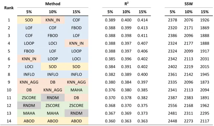
5.7.Overall performance of outlier algorithms ... 75

5.7.1.Hierarchical clustering ... 75

5.7.2.K-means clustering ... 76

5.8.Understanding coherence and cluster results ... 77

5.9.Understanding removal percentage ... 82

5.10. Understanding advantages and disadvantages of outlier methods ... 82

6. Conclusion ... 85

7. Recommendations for future research ... 87

7.1.Connecting outlier detection and clustering ... 87

7.2.Connecting dimension reduction and clustering ... 87

8. References ... 88

9. Annex ... 92

9.1.Similarity matrices for datasets ... 92

9.2.Evaluation metrics for synthetic data treated with outlier methods ... 93

9.3.Comments on results for incoherent datasets ... 94

9.3.1.BreastCancerOriginal ... 95

9.3.2.ForestFires ... 98

9.3.3.BreastCancerDiagnostic ... 101

9.3.4.GesturePhase ... 104

9.4.Figures for incoherent results ... 107

9.4.1.BreastCancerDiagnostic ... 107

9.4.2.BreastCancerOriginal ... 113

9.4.3.ForestFires ... 119

9.4.4.GesturePhase ... 125

9.5.Figures for coherent results ... 131

viii

9.5.2.Ionosphere ... 137

9.5.3.HeartDisease ... 143

9.5.4.Frogs ... 149

ix

ABBREVIATIONS

ABOD Angle-based Outlier Detection

COF Connectivety-based Outlier Factor

CRISP-DM Cross-industry standard process for data mining

DB Distance-based Outlier

FBOD Feature Bagging Outlier Detection

INFLO Influenced Outlierness

kNN k-nearest neighbor

LOCI Local Outlier Correlation Integral

LOF Local Outlier Factor

LOOP Local Outlier Probability

MAHA Mahalanobis Distance

RNDM Random

SOD Subspace Outlier Degree

SSB Sum of Squares Between

SST Sum of Squares Total

SSW Sum of Squares Within

1

1. INTRODUCTION

1.1. B

The discipline of data mining has in recent years seen a significant increase in research contributions, making it a constant updating field of science. For data mining, unsupervised learning is the discpline of gaining insights in unlabeled data by the means of different tools, usually following a data mining process such as CRISP-DM (Shearer, 2000), SEMMA (SAS, 2006) or KDD (Fayyad, Piatetsky-shapiro, & Smyth, 1996). Among the tools available in unsupervised learning, clustering is one of the most frequent used. Following the above-mentioned data mining processes, data preparation/modification/preprocessing (mentioned respectively to the papers) is executed prior to modelling, as one cannot model better than data allows. For data preparation, the task of detecting and treating outliers is important, for clustering to return optimal results.

However, the task of detecting outliers is subject to discussion as it is a abstract question defining what an outlier is. Moreover, no universally accepted approach to outlier detection with regards to clustering results has been developed.

With the ever-expanding field of literature, several authors have over time developed different outlier detection methods, claiming to have developed the single solution or algorithm that produce the best outlier detection within a certain data domain (Filzmoser, Maronna, & Werner, 2006; H.-P. Kriegel, Kröger, Schubert, & Zimek, 2009; B. Tang & He, 2017). However, no research has been done connecting outlier detection to optimized clustering results.

1.2. P

The no free lunch theorem states that no single algorithm produce the best result across all mathematical or computational problems. The same applies for clustering and outlier detection, where some clustering algorithms, such as DBSCAN (Ester, Kriegel, Xu, & Miinchen, 1996), have built-in exclusion of noisy objects, while other algorithms cannot deal with outliers.

Among the most used clustering algorithms, both k-means and hierarchical clustering lack properties to deal with outliers. Thus, as with any modelling problem, it is crucial to identify outliers for the clustering to return satisfying results, and based on allowance, either remove the outliers or reassign them after applied clustering. Returning to the no free lunch theorem, it is unknown how k-means and hierarchical

2 clustering excel in collaboration with certain outlier detection methods, and within what domains of data the two clustering algorithms have their respective advantage. This leads to following identified issues;

 Neither k-means nor hierarchical clustering is suitable for all kinds of datasets  Neither k-means nor hierarchical clustering can detect and deal with outliers Leading to the problem:

 The definition of an outlier is abstract. Depending on properties of data, it can be based on statistical tests, based on proximity, based on an algorithm, labeled or scored.

1.3. R

The main objective of this thesis is to contribute to the literature of data mining and create insight in outlier detection with regards to improved clustering performance. To achieve this goal, the main research question to be answered in this thesis is:

 How can outlier detection improve clustering results for k-means and hierarchical clustering? As implied in main research question, the thesis deals with two kinds of algorithms: outlier detection algorithms and clustering algorithms. The thesis is divided in to a theoretical part discussing tools identified in a literature review and a practical part applying the identified literature to data. To answer the main research question, a set of sub questions are formulated:

1. What is outlier detection and which tools does the literature provide?

Building foundational knowledge for the faced issue, this question serves to understand the nature of outlier detection and identify and understand the functionality of the outlier detection methods.

2. What is clustering, what are the objectives and how are clustering results evaluated?

To understand clustering and its objectives, a second literature review chapter will discuss the literature and describe the two clustering algorithms k-means and hierarchical clustering, later moving them on to the process of applied clustering. To understand how clustering objectives are quantified, clustering evaluation is also discussed.

3 3. How do outlier detection methods perform when comparing cluster results for data treated with

different outlier detection methods?

This question is approached from a practical perspective and deals with the actual research results by applying theory to given data. The question of performance will be quantified from the perspective of clustering objectives identified in question two. This thesis aims contribute to research by creating an understanding of advantages and disadvantages of outlier detection, for different clustering algorithms, for different datasets. If results return improved performance, it is expected that this thesis can help create an understanding of combinations of algorithms powerful for improved clustering performance.

1.4. S

Chapter 1 outlines the motivational background for the thesis and the scope of reasearch. Any discussion raised in the thesis serves the overall purpose of answering the research question stated in this chapter. Chapter 2 contains the general methodological framework of the thesis and describes the approach of answering the research question. It highlights how literature is discussed and literature is illustrated with practical cases. It also lists the general steps of applying theory of outlier detection and clustering to different datasets.

Chapter 3 presents the identified literature and is divided into three sections. The first section discusses the methodology for identification of literature. The second section deals with outlier detection and maps the contributions of literature until now. The literature is thoroughly described for the reader to understand technicalities. The third section deals with clustering and covers the topic by discussing objectives, tools and evaluation. Objectives of clustering are discussed with identified literature and serves to create a unified approach for later evaluation of clustering results. Evaluation of clustering results are described and discussed with identified evaluation metrics. A practical example is given for the reader to understand how evaluation metrics differ and to understand their respective advantages and disadvantages.

Chapter 4 describes the modelling methodology for applying theory to datasets. The first section discusses the selection of the datasets subject to applied theory. The importance of diversity in selected data is emphazised to answer the research question. The methodology for application of outlier detection and

4 clustering to selected datasets is detailed in the second section. Finaly, coherence for evaluation metrics is discussed in the third section.

Chapter 5 presents and discusses the results. It is described how the large amount of produced metrics are handled for the reader to understand the overall result. Results for datasets are divided in two categories: positive results with improved clustering performance, and dubious results with questionable performance.

Chapter 6 presents the overall conclusion with respect to the research question. The conclusion highlights the outcome for the two groups of datasets and discusses major findings.

5

2. METHODOLOGICAL FRAMEWORK

2.1. L

For the theoretical part dealing with outlier detection a literature review is conducted. The overall objective of the literature review is to identify secondary sources and map the current contributions to the discipline of outlier detection. The literature review strives to identify the most recognized algorithms to limit the number of algorithms applied to data, as testing every algorithm will create an unnecessary redundant long thesis. Furthermore, methodology for identification of literature is discussed at the beginning of the literature review chapter. To understand the nature of outlier detection and functionality of the outlier detection tools, the literature review contains discussions on a theoretical and practical level.

The theoretical discussion deals with the definition of an outlier and is rather philosophical. The literature is described from its early stages and discuss how the definition of an outlier has changed over time. The intuition of outlier detection, for identified approaches, is discussed for the reader to follow researchers’ reasoning of their respective suggested technical approaches.

The practical discussion includes illustration examples of data developed by the respective authors in order to understand technicalities of the theory and to elaborate on advantages and disadvantages of the reviewed approaches. Focus is on four different properties: applicability, method input parameters, method output and overall completeness

 Applicability is the extent to which an outlier detection method can deal with datasets of different characteristics.

 Method input parameter is the subjective input parameters that algorithms use as an input to judge ‘outlierness’.

 Method output is the output each method assigns to observations, binary (‘outlier’/’inlier’) or continuous (‘outlierness’).

 Overall completeness is the method’s completeness of ability to identify outliers.

As non-labeled data is used in clustering (data without an attribute categorizing observations into ‘outlier’/’inlier’), the thesis leaves out discussions about supervised scenarios for outlier detection.

6

2.2. L

The literature review on clustering aims to discuss the objectives of clustering and how clustering results are evaluated. For objectives of clustering, literature is identified from several authors, providing their respective definition of objectives. The definition of objectives is discussed to create a unified definition, later quantified when discussing cluster evaluation.

For evaluation of clustering, quantification of clustering objectives is conducted with evaluation metrics. Advantages and disadvantages of evaluation methods are discussed along with a discussion of how different evaluation metrics have mutual dependence. Furthermore, a set of practical illustrations is provided.

2.3. A

Finally, to quantify how outlier detection can improve clustering results, the following steps are executed: - Step 1: Dataset is selected.

A wide range of datasets with different properties are selected for analysis. It is striven that datasets vary in number of attributes (variables) and observations, vary in composition of categorical and continuous attributes and vary in statistical characteristics. Furthermore, a discussion of selection of datasets is conducted in the analysis.

- Step 2: Outlier detection method is applied, and top-n % outliers are removed

For each dataset, prior to applying clustering algorithms, selected outlier detection methods are applied for removal of top-n outliers. For equal comparison across outlier detection algorithms, top 5%, 10% and 15% outliers are removed based on the algorithms ‘outlierness’ output for observations. Simultaneously, 5%, 10% and 15% random selected observations are removed, for later comparison of clustering results. Removal of random selected observations is conducted to evaluate whether outlier removal improves clustering results at all. That is, comparing apples with apples.

- Step 3: Clustering is applied to treated dataset and evaluated

For each treated dataset, clustering algorithms are applied, and results are discussed based on the clustering evaluation criteria identified. It is summarized how outlier detection and clustering algorithms excel in combination for datasets of different properties.

7

“

“

“

“

“

“

“

“

“

“

3. LITERATURE REVIEW

The term outlier was introduced in 1969 when Grubbs (Grubbs, 1969) argued that “an outlying observation, or ‘outlier’, is one that appears to deviate markedly from other members of the sample in which it occurs”. Following Grubbs (1969), Hawkins (1980) argued that “an outlier is an observation which deviates so much from the other observations as to arouse suspicions that it was generated by a different mechanism” while Barnett and Lewis (1994) defined an outlier as “an observation or subset of observations which appears to be inconsistent with the remainder”. However, prior to Grubbs and Hawkins, Benjamin Pierce (1852) and Charles Pierce (1873) published papers respectively mentioning: “Criterion for the Rejection of Doubtful Observations” and “On the Theory of Errors of Observations”, discussing observations with deviating characteristics. Thus, the idea of observations with outlying characteristics has existed for a longer period.

There is not a single definition of an outlier, making it subject to discussion. However, there is a consensus that an outlier in some way has deviating characteristics. For the remaining thesis, an inlier is defined as the contradiction of an outlier, meaning that an inlier does not have deviating characteristics:

An outlying observation, or ‘outlier’, is one that appears to deviate markedly from other members of the sample in which it occurs

- Grubbs (1969) An outlier is an observation which deviates so much from the other observations as to arouse suspicions that it was generated by a different mechanism

- Hawkins (1980) An observation or subset of observations which appears to be inconsistent with the remainder

- Barnett & Lewis (1994) An outlier is an observation distant to other observations

– Knorr & Ng (1997) An outlier in a set of data is an observation or a point that is considerably dissimilar or inconsistent with the remainder of the data

8

“

“

3.1. M

The discipline of outlier detection has been thoroughly researched. ‘Outlier detection’ generates 57.000 results on ScienceDirect, making it impossible to review the literature article by article. To create an overview of the scope of literature, following steps are executed:

1. The most well-cited meta studies (review articles) within the field of outlier detection are downloaded from ScienceDirect, based on the keyword ‘outlier’.

2. The outlier detection methods, from the review articles, are compared across articles to identify the most frequent reviewed methods, approaches and authors (domain experts).

3. The identified methods are compared with general search machine results and Wikipedia pages for outlier detection1 _{and anomaly detection}2 _{to get a consensus of the identified literature.}

4. The reviewed literature, identified in the review articles, is downloaded from ScienceDirect with the most recent first. For each article, a chapter describing the current literature until publication of the respective article, is inspected.

5. If the inspected chapter refers to literature not identified earlier, the newly identified literature is downloaded.

With the above-mentioned approach for literature identification, a ‘history’ of evolution in the discipline of outlier detection is mapped. The downside for this approach is the lack of recent literature as a result of missing review papers.

Following criteria and considerations are put in place while executing previously described process:  The identified literature must be applicable to both discrete and continuous data.

This criterion is created to solely identify universal applicable methods, avoiding literature dealing only with certain types of data (e.g. time series or spatial data). The only exemption for this criterion is the

1 _{https://en.wikipedia.org/wiki/Outlier}

9 early literature of outlier detection (statistical test) which is included to create a fundamental understanding of outlier detection and its origin.

 The identified literature must be original research proposing an approach to outlier identification not previously seen

This criterion is created to avoid literature suggesting how to deal with outlier detection within a certain field (e.g. logistic systems, healthcare, fraud systems) by applying an already developed method to a practical case.

 The identified literature must be well cited (≥50) and/or preferably from a notable author within the discipline

This criterion is created to avoid spending a disproportionate amount of time compared to importance of the literature. Literature without important contributions to the discipline generally fails to be cited.

 The theory in the identified literature must have a continuous element

This criterion is created with respect to the methodology of removing top-n % of outliers based on outlier method output. The identified literature can have a binary output, as a threshold for observations to be identified as outliers, if the threshold is based on an underlying continuous element returning outlierness for observations.

3.2. O

Table 1 highlights 29 identified crucial papers. The literature is divided into approaches and shows the number of citations per paper. The number of citations is a conservative estimate based on numbers from the source, mostly being ScienceDirect or ResearchGate.

As with many fields of science, the approaches are characterized by one or more authors introducing a new approach to a problem, followed by other researchers adopting the approach for improvement of the theory. Literature dealing with distance-based or more complex approaches tends to propose a new algorithm for outlier detection, followed by one or more papers suggesting a modified algorithm for computational optimization.

10 With respect to the research question and the limitations stated earlier in this thesis, the literature solely dealing with computational optimizations is not discussed in this literature review.

Authors Paper name Approach Citations

Grubbs (1950) Sample Criteria for Testing Outlying Observations Statistical test 644 Wilk, Gnanadesikan

(1968) Probability Plotting Methods for the analysis of data Statistical test 728 Grubbs (1969) Procedures for Detection Outlying Observations in Samples Statistical test 1575 Gnanadesikan,

Kettenring (1972) Robust Estimates, Residuals, and Outlier Detection with Multiresponse Data Statistical test 558 Tukey (1977) Explorative Data Analysis Statistical test 16676 Garrett (1989) The chi-square plot: A tool for multivariate outlier recognition Statistical test 61 Iglewicz, Hoaglin

(1993) How To Detect and Handle Outliers Statistical test 580 Filzmoser, Garrett,

Reimann (2005) Multivariate Outlier Detection in Exploration Geochemistry Statistical test 190 Vanderviere, Huber

(2008) Adjusted Boxplot for Skewed Distributions Statistical test 169 Knorr, Ng (1997) A Unified Approach for Mining Outliers Distance-based 57 Knorr, Ng (1998) Algorithms for Mining Distance-Based Outliers in Large _Datasets Distance-based 979 Knorr, Ng (1999) Finding Intensional Knowledge of Distance-Based Outliers Distance-based 310 Ramaswamy, Rastogi,

Shim (2000) Efficient Algorithms for Mining Outliers from Large Data Sets Distance-based 921 Angiulli, Pizzuti

(2002) Fast Outlier Detection in High Dimensional Spaces Distance-based 235 Hautamaki,

Kärkkäinen, Fränti (2004)

Outlier Detection Using K-nearest Neighbour Graph Distance-based 50 Fan, Zaïane, Foss, Wu

(2006)

A Nonparametric Outlier Detection for Effectively Discovering

Top-N Outliers from Engineering Data Distance-based 56 Zhang, Hutter, Jin

(2009) A New Local Distance-Based Outlier Detection Approach for Scattered Real-World Data Distance-based 198 Breuning, Kriegel, Ng,

Sander (2000) LOF: Identifying Density-Based Local Outliers Density-based 1741 Jin, Tung, Han

11

Authors Paper name Approach Citations

Tang, Chen, Fu, Cheung (2002)

Enhancing Effectiveness of Outlier Detections for Low Density

Patterns Density-based 146

Papadimitriou, Kitagawa, Gibbons, Faloutsos (2003)

LOCI: Fast Outlier Detection Using the Local Correlation

Integral Density-based 482

Jin, Tung, Han, Wang

(2006) Ranking Outliers Using Symmetric Neighborhood Relationship Density-based 139 Latecki, Lazarevic,

Pokrajac (2007)

Outlier Detection with Kernel Density Functions Density-based 84 Kriegel, Kröger,

Schubert, Zimek

(2009) LoOP: Local Outlier Probabilities Density-based 115 Schubert, Zimek,

Kriegel (2014)

Generalized Outlier Detection with Flexible Kernel Density

Estimates 3 Density-based 44

Lazarevic, Kumar

(2005) Feature Bagging for Outlier Detection High-dimensional 187 Kriegel, Schubert,

Zimek (2008) Angle-Based Outlier Detection in High-Dimensional Data High-dimensional 150 Kriegel, Kröger,

Schubert, Zimek (2009)

Outlier Detection in Axis-Parallel Subspaces of High

Dimensional Data High-dimensional 68 Kriegel, Kröger,

Schubert, Zimek (2011)

Interpreting and Unifying Outlier Scores High-dimensional 60 Table 1: Identified literature

For the identified literature a trend is observed. Generally, the early literature mentions outliers in a statistical testing context, where the discipline of outlier detection serves the purpose of removing outliers to improve hypothesizes testing and statistical significance. Early literature perceives outlier detection as the probability of an observation belonging to a distribution, whereas more recent literature mentions outliers in a context of discovering anomalies in large datasets. Furthermore, more recent literature is largely divided in to distance-based, density-based and high-dimensional approaches. Common for this literature is the abandonment of probability theory in favour of multidimensional

12 proximity. Thus, with the improvement and adoption of computational power, scope has moved from statistical testing, mostly a univariate discipline, to data mining, a multivariate discipline.

To have a unified approach and definition of outlier detection for the remaining literature review, outlier detection is defined as follows:

 Outlier detection is the discipline of identifying observations with deviating characteristics, by the means of different approaches (e.g. statistical test, density-based approach).

3.2.1. Statistical Z-test

Statistical test for outliers assumes an underlying normal distributed population (Grubbs, 1969), also called parametric test, meaning that a set of parameters are assumed fixed. Non-parametric test differs from parametric test by having a set of parameters that can vary in numbers and does not necessarily rely on an assumed underlying distribution.

Grubbs argued that statistical outliers should be identified as observations that “would exceed the ‘critical value’ based on random sampling theory”, and that critical value “is generally recommended […] a low significance level, such as 1%”.

A simple univariate approach to test if observations exceed a critical value is the Z-score:

𝑍 =𝑋 − 𝑋

𝑆𝐷

where 𝑋 is the sample mean and 𝑆𝐷 is the sample standard deviation.

The Z-score method is based on the idea that 𝑋 follows a normal distribution, 𝑁(𝜇, 𝜎 ), and Z-scores follow a standard normal distribution, 𝑁(0,1). The Z-score reflects the number of sample standard deviations observation 𝑋 differs from 𝑋. An outlier is identified as |𝑍| > 3, based on the idea that 99.7% of the observations are within 3 standard deviations from the mean in a normal distribution and anything greater would be rejected as an outlier belonging to a different distribution.

However, the Z-score, using the standard deviation, lacks robustness. As the standard deviation can be affected by extreme values, meaning that observations that are considered outliers in a sample, are identified as inliers, when an even more extreme observation enters the sample. Thus, the standard deviation possesses a weakness, as it is a measure of deviation in a sample, based on the sum of deviations from the mean including the very outlying observations the user is trying to identify.

13

3.2.2. Robust statistics

To overcome this issue, Iglewicz & Hoaglin (1993) suggested an approach based on robustness. Robust statistics focus on the median as a measure of central tendency, while the mean is viewed as a measure vulnerable to extreme values. To replace the standard deviation, Iglewicz & Hoaglin (1993) introduced the absolute deviation of the median (MAD):

𝑀𝐴𝐷 = 𝑚𝑒𝑑𝑖𝑎𝑛(|𝑋 − 𝑋|) where 𝑋 is the sample median.

The modified Z-score approach suggested is:

𝑀 =0.6745(𝑋 − 𝑋)

𝑀𝐴𝐷

where 0.6745 is equal to the number of standard deviations having 50% of the observations within in a normal distribution. It was suggested that observations with |𝑀 | > 3.5 should be identified as outliers.

3.2.3. Tukey’s boxplot

With his book Explorative Data Analysis, Tukey (1977) presented a visual approach for exploring data and provided the boxplot as a simple approach to display properties of a distribution. Having no underlying assumptions of a normal distribution, the method is non-parametric. Tukey’s boxplot has since then been widely accepted as a default method to identify outliers in univariate data.

Tukey argued that outliers are identified using inner and outer fences:

𝑙𝑜𝑤𝑒𝑟 𝑖𝑛𝑛𝑒𝑟 𝑓𝑒𝑛𝑐𝑒 = 𝑄 − 1.5(𝑄 − 𝑄 ) and 𝑢𝑝𝑝𝑒𝑟 𝑖𝑛𝑛𝑒𝑟 𝑓𝑒𝑛𝑐𝑒 = 𝑄 + 1.5(𝑄 − 𝑄 )

𝑙𝑜𝑤𝑒𝑟 𝑜𝑢𝑡𝑒𝑟 𝑓𝑒𝑛𝑐𝑒 = 𝑄 − 3(𝑄 − 𝑄 ) and 𝑢𝑝𝑝𝑒𝑟 𝑜𝑢𝑡𝑒𝑟 𝑓𝑒𝑛𝑐𝑒 = 𝑄 + 3(𝑄 − 𝑄 )

where 𝑄 and 𝑄 are the first and third quantiles respectively, and 𝑄 − 𝑄 is the interquartile range (IQR). Any observation between the inner and outer fences are identified as moderate outliers, and observations lower than the lower outer fence or greater than the upper outer fence are identified as severe outliers.

Tukey’s boxplot (Tukey, 1977) has great properties in univariate data, being a robust statistical tool based on quartiles while graphically reflecting the characteristics of a distribution such as distance between mean and median, length of tails, skewness and outliers. Although Vanderviere & Huber (2008) criticized

14 Tukey’s boxplot (Tukey, 1977) for lack of properties to deal with skewed data, leading to the adjusted boxplot, the boxplot approach has its greatest shortcomings in multivariate data.

3.2.4. Mahalanobis distance

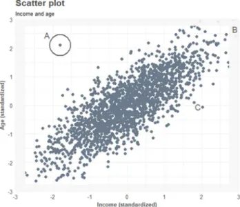
The scatterplot exhibits the observations of two variables (X, Y) in a two-dimensional space. When a point deviates significantly from the cloud of points of the other observations, it may indicate an outlier. To quantify its deviation, Euclidean distance is useful to derive the distance from the center of gravity (0, 0), to the atypical observation. Euclidean distance is defined as:

𝐷(𝑞, 𝑝) = (𝑞 − 𝑝 )

where 𝑞 and 𝑝 are the coordinates of observations and 𝑖 is the number of the respective dimension. Thus, to calculate the distance to the center of gravity for a standardized dataset, where center of gravity is given by 𝜇⃗ = 0

0 , the coordinates are squared, summed and square rooted.

However, applicability of Euclidean distance in correlated data has weaknesses. For example, in Figure 1, it identifies observation A and B with a distance from the center of gravity of 2.76 and 3.88, respectively, expressing greater outlierness for observation B than observation A. That is despite of observation B following the correlated pattern of the data, having less deviating characteristics than observation A.

15 To deal with outliers for regression and multivariate data, it is necessary to take the covariance of the variables into account. For that, Mahalanobis distance (Mahalanobis, 1936) is useful. Mahalanobis distance identifies a set of vectors, corresponding to the number of dimensions, with the first vector explaining the most variance, which in this case is the vector fitting the correlated pattern. The second vector explains the second most variance and is perpendicular with the first vector.

Mahalanobis distance is defined as:

𝑀𝐷(𝑥⃗) = 𝑋⃗ − 𝜇⃗ 𝑆 (𝑋⃗ − 𝜇⃗)

where 𝑋⃗ is a vector of observations with mean values given by the vector 𝜇⃗ and 𝑆 is the inverse covariance matrix for variables.

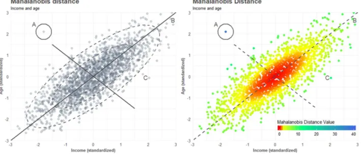
For the data in Figure 1, a covariance matrix 𝑆 = 1.00 0.80

0.80 1.00 express a correlation of .80 between the two variables. For demonstration purpose, Mahalanobis distance is visualized in Figure 2.

Figure 2: Mahalanobis distance visualized with standard deviations (left) and value (right)

Inspecting Figure 2, the standard deviation for the vectors follows the correlated pattern of the data, meaning that 68-95-99.7 confidence intervals, with 1, 2 and 3 standard deviations respectively, is given by an ellipse shape. Observations deviating on the second vector have a greater distance from the center of gravity, as they deviate the correlated pattern of the data.

16 Observation B is considered the most outlying observation from center of gravity based on Euclidean distance, but does not differ substantially from observation C with Mahalanobis distance. Observation A is by far to be considered the observation with the most outlying characteristics following Mahalanobis distance. Although using Mahalanobis distance for outlier detection is not based on a certain threshold, a probability density plot by Mahalanobis distance will show the observations deviating greatest in the tail. Mahalanobis distance is applicable to datasets characterized by continuous data with collinearity and should mostly be used within this specific domain. As with univariate data, usage of robust estimates for mean and standard deviation in Mahalanobis distance, will perform better when working with correlated data with extreme outliers. Working with uncorrelated data, non-robust Mahalanobis distance will perform worse than Tukey’s boxplot, considering that Tukey’s boxplot is robust, hence not being sensitive to extreme outliers. Furthermore, Mahalanobis distance will fail when working with categorical variables, as Mahalanobis distance is based on covariance and means.

3.2.5. Q-Q plot and Chi-square plot

The Q-Q plot (quantile-quantile plot), was suggested (Wilk & Gnanadesikan, 1968) as a tool for investigating if a sample distribution follows a normal distribution. The Q-Q plot has versions with different properties, the most popular being the version plotting a given sample distribution against a theoretical standard normal distribution 𝑁(0,1). For that version, data is ordered in increasing order (𝑋 < 𝑋 < . . . < 𝑋 ), and a standard normal distribution is divided in to 𝑛 + 1 areas, with 𝑛 being the number of observations in a sample, with each area having equal probability density. The 𝑖th ordered observations are in increasing order plotted against the 𝑡ℎ quantile for a standard normal distribution, reflecting if the sample follows a normal distribution.

The Q-Q plot can technically plot any sample distribution against another distribution, making it a great tool to discover outliers in the tails of a sample distribution, if plotted against an appropriate distribution. The Q-Q plot has its strength in univariate data and for multivariate data with a maximum of two dimensions. As it requires a pairwise inspection, variable by variable, it is time consuming for multidimensional data (>2d) and to some extent also subjective.

For a more effective outlier detection method following same philosophy of quantile inspection, Garrett (1989) suggested to use the chi-square plot. The chi-square plot plots the squared Mahalanobis distance against the quantiles of a chi-square distribution (𝑋 ), with 𝑝 degrees of freedom, allowing the user to

17 inspect a multivariate distribution against a theoretical distribution, leading to identification of observations deviating from multivariate normality in the tails. The procedure allows the user to delete the most extreme observations, until the observations fall into a straight line. This method is more effective than pairwise inspection of multiple distributions, as it essentially is a multidimensional Q-Q plot.

3.2.6. Distance-based approaches

Going from statistical testing to distance-based approaches for identifying outliers, scope in the literature changes from probabilities of an observation belonging to a distribution, to knowledge discovery in large datasets, also called data mining. With different philosophy of distance and deviation, data mining methods leave out centrality and dispersion measures such as mean, quantiles and standard deviation, characterized by statistical testing.

Ramaswamy, Rastogi, & Shim (2000) argued that the main problem with statistical testing is that ‘the user might not have enough knowledge about the underlying data distribution’ and the main benefit of distance-based approaches is that ‘it does not require any apriori knowledge of data distributions that the statistical methods do’.

Knorr & Ng (1997) argued that despite of all the statistical test available for outlier detection, ‘there is no guarantee of finding outliers’ as ‘there might not be any test developed for a specific combination or because no standard distribution can adequately model the observed distribution’. Thus, the desire with distance-based approaches is to replace assumptions of underlying data distributions with observed data distributions.

3.2.6.1. DB Outlier

Knorr & Ng (1997) introduced distance-based approaches by focusing on neighborhood of observations. The distance-based methodology was defined as ‘An object O in a dataset T is a UO(p, D)-outlier if at least fraction P of the objects in T are > distance D from O’. They suggested a rather simple method called DB-outlier.

Let the distance 𝐷, which can take any distance input, be a radius from object 𝑂 in a two-dimensional space. The distance 𝐷 is set to 1.5. Let the fraction parameter 𝑃, which can take any input between 0 and 1, be set to 0.05 or 5% of dataset 𝑇. Let observations within object 𝑂’s neighborhood, given distance measure 𝐷, be labeled as observations 𝑄 . If the proportion of 𝑄 within observation 𝑂’s neighborhood,

18 over the total number of observations in dataset 𝑇, is less than the fraction parameter 𝑃, observation 𝑂 is considered an outlier and vice versa. Outliers are then given by:

𝑂𝑢𝑡𝑙𝑖𝑒𝑟𝑠(𝐷, 𝑃) =(𝑄|𝑑𝑖𝑠𝑡(𝑂, 𝑄) < 𝐷)

𝑇 ≤ 𝑃

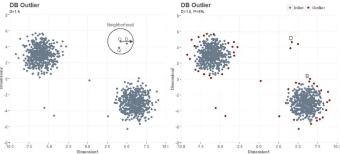
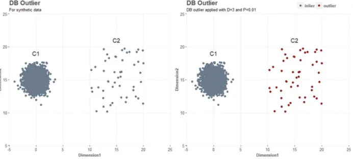
Inspecting Figure 3, which was created for demonstration purposes, the distribution for dimension 1 and 2 is not normally distributed, but rather bimodal. The observation 𝑂, of which DB-outlier method is demonstrated, would hide in the bimodal peaks in the distributions for dimension 1 and 2. For left plot, observation 𝑂 has a neighborhood given by distance 𝐷, in which two neighboring observations 𝑄 are identified. The proportion of neighboring observations 𝑄 is less than fraction parameter 𝑃 of 0.05, or 5% of data. Observation 𝑂 is therefore identified as an outlier.

Figure 3: Distance-based outlier approach (left) and result (right)

Where statistical test is based on assumptions of certain underlying distribution and centrality, leading to lack of properties to deal with high-dimensional data, the distance-based approach DB-outlier, performs well to identify anomalies in datasets characterized by many dimensions and non-normal distributions. Being the first approach suggested for outlier detection within the discipline of data mining, the model builds a solid foundation based on concept of distance and neighborhood.

The theory is however not completely fit for outlier detection in multivariate data, as it has two major shortcomings. The first shortcoming is the binary output. Observation 𝑂 and observation 𝐵 (see: Figure 3) are both identified as outliers, but do not have the same deviating characteristics. Observation 𝐵 is

19 close to one of the two gaussian clusters, while observation 𝑂 is distant to other observations. Thus, the binary output does not provide the user with an idea of outlierness for observations. The second shortcoming is the subjective threshold of parameter 𝑃 and the distance 𝐷, leaving the user with no options but to loop over different input parameters. A large distance 𝐷 and low 𝑃 will only identify the most deviating observations, whereas small distance 𝐷 and high 𝑃 will identify more observations as outliers. A solution to both shortcomings is to omit parameter 𝑃, and let the user judge each observation by the proportion of observations within its neighborhood, over the total number of observations, providing an output between 0 and 1.

3.2.6.2. K Nearest Neighbor

As with a lot of pioneering research, the DB-outlier method is the first within its field, but others adopted the idea of distance and neighborhood to improve the theory.

Ramaswamy, Rastogi, & Shim (2000) suggested an algorithm called ‘k-NN’, based on the distance to 𝑘 nearest neighbor for each observation 𝑝 in dataset. The distance measure for observation 𝑝 to 𝑘 nearest neighbors is noted as 𝑑𝑖𝑠𝑡 (𝑝). The idea is that observations with low 𝑑𝑖𝑠𝑡 (𝑝) have a dense neighborhood, meaning that observation 𝑝 does not have deviating characteristics. Top 𝑛 observations with high 𝑑𝑖𝑠𝑡 (𝑝) have sparse neighborhoods and deviating characteristics and will be considered outliers.

The k-NN approach is intuitive and provides a measure of ‘outlierness’ allowing the user to judge how deviating an observation is, hence avoiding binary output. Furthermore, different measures of distance can be taken, such as Euclidean distance and Manhattan Distance, increasing the flexibility of the algorithm.

However, as well as it can be an advantage to have continuous output and many input options, it also leaves the user with a subjective decision making. The subjective difficulties consist of setting a threshold of 𝑑𝑖𝑠𝑡 (𝑝) for top 𝑛 observations to be identified as outliers and setting a factor of 𝑘.

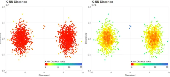
For demonstration purposes, Figure 4 is created. The left plot has 𝑘 = 1 and right plot has 𝑘 = 10. With 𝑘 = 1, each observation 𝑝 will only return distance to nearest observation, failing to identify a group of close observations in an outlying cluster. The three observations seen in between the two major gaussian clusters of observations in Figure 4 are therefore identified as inliers. If 𝑘 is large (such as 𝑘 = 50% 𝑜𝑓 𝑛), it will produce less variance in the output vector of 𝑑𝑖𝑠𝑡 (𝑝). Less variance equals more similar 𝑑𝑖𝑠𝑡 (𝑝) for observations, making it more difficult to identify the outliers with the strongest

20 outlierness. This leads to a trial and error process of iterations over different factors for 𝑘, further increasing subjectivity when eventually choosing threshold.

Figure 4: K-NN distance for k=1 (left) and k=10 (right)

To limit the issue of subjectivity, Angiulli & Pizzuti (2002) adopted the k-NN methodology but suggested an algorithm aggregating the k-NN with 𝑘 as an input range. With 𝑘 = {4, 5, . . , 10}, the results of 4NN, 5NN, … and 10NN is aggregated. The aggregated measure is a weight and is given by:

𝑤 (𝑝) = 𝑑𝑖𝑠𝑡(𝑝, 𝑛𝑛 (𝑝))

where 𝑛𝑛 is the 𝑖th nearest observation/neighboring of observation 𝑝, given parameter 𝑘.

The algorithm leaves the user with less subjectivity and it gives a simpler output and smoother result of outlierness for observations.

Hautamaki & Ismo (2004) adopted the k-NN theory and proposed an algorithm combining network theory and k-NN, naming it k-NN Graph. It was suggested to calculate the in-degree for each observation, given 𝑘 nearest neighbors. An observation with sparse neighborhood has low in-degree as few other observations connects to it due to missing proximity, and vice versa. If the in-degree for an observation is less than a threshold 𝑇, it is considered an outlier.

Inspecting Figure 5, which was created for demonstration purposes, left plot shows the links of observations identifying neighbors by ‘linking’. With 𝑘=3, observation A connects to its three nearest

21 neighbors, being observation B, C and D, giving each observation one in-degree. The closest observation in the neighborhood of observation A, is observation B. Observation B connects to observation C, D and E as the closest neighboring observations, leaving no in-degree for observation A. The same accounts for observation C and D, meaning observation A is not in the neighborhood of any observation when 𝑘=3. Thus, observation A is identified as an outlier, when the threshold 𝑇 is set to ≤ 2.

Figure 5: K-NN Graph for synthetic data with network (left) and classification (right)

As with DB-outlier, the output for K-NN Graph is a binary label. Again, it is concluded that a small 𝑘 will fail to identify an outlying cluster of observations, as the observations in the given cluster simply would connect to each other with in-degrees. Although not suggested by Hautamaki et al. (2004), the eigenvector centrality metric from network theory is applicable to overcome this issue. The eigenvector centrality returns a number indicating how well-connected an observation is to other well-connected observations, exposing an outlying cluster of observations with low in degree values. Again, it is concluded that the threshold should be removed if the user wants to inspect the outlierness for each observation to provide an idea of how deviating observations are.

3.2.7. Density-based approaches

Density-based approaches were introduced by Breunig, Kriegel, Ng, & Sander (2000), following the introduction of distance-based approaches. As with distance-based approaches, it was argued that outlier detection based on statistical test has major drawbacks in data mining as most methods are univariate and the underlying distribution often is unknown. However, it was also argued that the distance-based

22 approaches lacked properties to deal with neighborhoods of different densities, due to being a ‘global’ outlier detection method. A ‘global’ methods means the entire dataset is taken in to account when comparing observations for outlierness. For DB-outlier, the amount of observations in the neighborhood given by distance 𝐷, is compared to the total amount of observations in dataset 𝑇. For various variants of k-NN, distance is compared to the distance to nearest neighborhood for every other observation in dataset. Thus, the global methods lack properties to identify outliers in neighborhoods of different densities.

Inspecting Figure 6, which was created for demonstration purposes, it is observed that observations in gaussian cluster 𝐶1 have a dense neighborhood and are identified as inliers while observations in cluster 𝐶2 are identified as outliers although the observations do not have deviating characteristics, relatively to their neighbors, and although 𝑃 = 0.01, meaning that just 1% of observations within a distance of 3 is necessary to be an inlier.

Figure 6: Synthetic data (left) taken from Breuning et. al (2000) with DB outlier applied (right)

For an analogy with income and age, the philosophy of outlier detection for density-based approaches is to compare Warren Buffet with Bill Gates, Carlos Slim and other billionaires, leaving out global comparison with 99% of the remaining population. As an example, Mark Zuckerberg aged 32 is an outlier relatively to other billionaires, such as Warren Buffet, Bill Gates and Carlos Slim with an age of 86, 61 and 77, respectively.

23

3.2.7.1. Local Outlier Factor (LOF)

With more than 1.700 citations, Breunig, Kriegel, Ng, & Sander (2000) successfully introduced density-based approaches as a new domain in outlier detection. To identify outliers locally, it was argued that observations outlierness should be perceived relatively to the neighborhood, leaving out the global data distribution. The intuition is that outliers are identified as having different density in the neighborhood, when compared to the density in the neighborhood of neighboring observations.

An algorithm was proposed, taking only input parameter 𝑘, being the number of nearest neighbors to compare neighborhood density with. For each observation 𝑜 in dataset, the neighborhood boundaries, given parameter 𝑘, are defined as:

𝑟𝑒𝑎𝑐ℎ𝐷𝑖𝑠𝑡 (𝑜, 𝑝) = 𝑚𝑎𝑥{𝑘𝐷𝑖𝑠𝑡(𝑝), 𝑑(𝑜, 𝑝)}

meaning the most distant 𝑘 observation defines the boundaries of the neighborhood. As two or more observations can have equal distance to observation 𝑜, the number of observations within the neighborhood can be greater than 𝑘.

The density of the neighborhood is given by the local reachability density computed as:

𝑙𝑟𝑑 (𝑜) = 1/ ∑ ∈ ( )𝑟𝑒𝑎𝑐ℎ𝐷𝑖𝑠𝑡 (𝑜, 𝑝)

|𝑁 (𝑜)|

where |𝑁 (𝑝)| is the number of observations within the neighborhood, given a certain 𝑘. Thus, the local reachability is 1 over the accumulated distance from neighboring observations to observation 𝑜, over the number of observations in the neighborhood of observation 𝑜.

The local outlier factor (LOF) is then computed as:

𝐿𝑂𝐹 (𝑜) = ∑ 𝑙𝑟𝑑 (𝑝) 𝑙𝑟𝑑 (𝑜) ∈ ( ) |𝑁 (𝑜)| = ∑ ∈ ( )𝑙𝑟𝑑(𝑝) |𝑁 (𝑜)| /𝑙𝑟𝑑 (𝑜)

which is the average local reachability density for observations {𝑝 , 𝑝 , … , 𝑝 } in the neighborhood of observation 𝑜, divided by the local reachability density for observation 𝑜. A LOF close to 1 indicates equal neighborhood density relatively to neighboring observations, whereas a LOF significantly lower (e.g. 0.5) indicates relatively denser neighborhood. Significantly higher LOF-score, say 5, indicates relatively sparse neighborhood and outlierness.

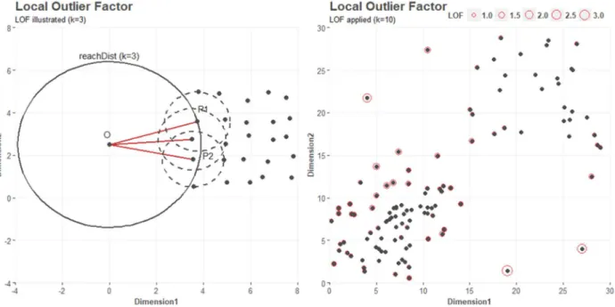
24 For demonstration purposes, the left plot in Figure 7 shows a sparse neighborhood for observation 𝑜, when 𝑘 = 3. Observation 𝑝 , 𝑝 and 𝑝 are closest neighbors to 𝑜, and all have denser neighborhoods, reflected by the size of the dashed 𝑟𝑒𝑎𝑐ℎ𝐷𝑖𝑠𝑡 for each 𝑝. The right plot shows two odd distributions, with small clusters of different densities. LOF is applied with 𝑘 = 10 and a LOF score is assigned to observations. Observations are identified with sparse neighborhood, relatively to neighbors, with LOF-scores >3. Thus, with its relative density methodology, LOF performs well in neighborhoods of different densities and provides a continous scoring output, enabling users to identify the observations with strongest outlierness.

Figure 7: LOF illustrated (left) with example (right) showing LOF-score for observations

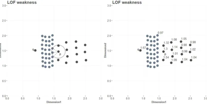
Density-based approaches was adopted (Jin, Tung, & Han, 2001; Jin, Tung, Han, & Wang, 2006), with the former concerning computational performance and the latter dealing with close clusters of different densities. The latter is of special interest as it is a contribution to the theory, optimizing outlier identificating for observations close to clusters of different densities. Jin, Tung, Han, & Wang (2006) criticised standard LOF by arguing that observations belonging to a sparse cluster, while being close to a dense cluster, will identify neighbors in the dense cluster for comparison. With neighbors in the dense cluster, the observation belonging to a sparse cluster will wrongly have a high outlier score assigned. For demonstration purposes, the left plot in Figure 8 contains observation 𝑞 as a local outlier and observaiton 𝑝 as an inlier in a sparse cluster. The plot reveals observation 𝑝 as identifying three closest

25 neighbors in the dense cluster. The right plot shows a LOF-score of 1.46 for observation 𝑝 as it compares neighborhood density with observations in the dense cluster. Thus, observation 𝑝 is identified as the second most outlying observation, with only observation 𝑞 having greater outlierness. Observation 𝑝 does not have deviating characteristics and is therefore incorrectly assigned with relatively great outlierness. To overcome this shortcoming, increasing 𝑘 can be a solution as well as it can further increase the problem. When increasing 𝑘, users do not know if bordering observations identifies more neighbors in different cluster with denser neighborhood or identifies neighbors in the cluster it belongs to.

Figure 8: Two close clusters in black and blue of different density (left) and LOF-score for observations (right)

3.2.7.2. Influenced Outlierness (INFLO)

For the above-mentioned shortcoming, an algorithm called influenced outlierness (INFLO) was proposed (Jin et al., 2006). The algorithm takes symmetric neighborhood relationship in to account and consideres an influenced space by the means of k-NN and the reverse nearest neighbor (RNN). The reverse nearest neighbor is described as an inverse relation in which other observations have spatial proximity to the observation subject to outlier identification. For simplification, we can return to Figure 5 demonstrating k-NN in-degree as suggested by Hautamaki & Ismo (2004). Observation A identifies observation B, C and D as neighbors when 𝑘 = 3, but observation B, C and D does not identify observation A as a nearest neighbor. Thus, observation A is a reverse neighbor of observation B, C and D.

26 Applying the analogy to the demonstrated case in Figure 8, observation 𝑝 has an inverse relationship with other observations in the sparse cluster, as these observations identify observation 𝑝 as a nearest neighbor. For a set of observations {𝑞 , 𝑞 , 𝑞 , … , 𝑞 } with an inverse relationship to observation 𝑝, the nearest neighbor of those will be identified, avoiding impact from the actual nearest neighbors. The influenced space for observation 𝑝 is then defined as 𝐼𝑆 (𝑝) = {𝑞 , 𝑞 , 𝑞 } where 𝑘 is the nearest neighbors parameter for the set of inverse relation to observation 𝑝. The average density of the influenced space for observation 𝑝 is given by:

𝑑𝑒𝑛 𝐼𝑆 (𝑃) =∑ ∈ ( )𝑑𝑒𝑛(𝑜)

|𝐼𝑆 (𝑃)|

where 𝑑𝑒𝑛(𝑜) is the density of the neighborhood for observations with inverse relationship {𝑞 , 𝑞 , 𝑞 , … , 𝑞 } to observation 𝑝 and |𝐼𝑆 (𝑃)| is the number of nearest neighbors. INFLO-score is then given by:

𝐼𝑁𝐹𝐿𝑂 (𝑝) =𝑑𝑒𝑛 𝐼𝑆 (𝑃)

𝑑𝑒𝑛(𝑝)

Observations with INFLO-score around 1 have similar neighborhood density, when compared with neighborhood density in the influenced space. Observations with INFLO-score greater than 1 have less dense neighborhood relatively to neighborhood density in the influenced space, indicating outlierness for observation 𝑝. Thus, INFLO and LOF have similar output properties for scoring outlierness.

3.2.7.3. Connectivity-based Outlier Factor (COF)

J. Tang, Chen, Fu, & Cheung (2002) adopted the density-based approach and argued that measuring change in density may rule out outliers close to some non-outliers patterns that have low density. That is, outliers are difficult to detect in areas of low density, and choosing a large 𝑘 may result in entire clusters of low density to be identified as outliers. To overcome this issue, J. Tang, Chen, Fu, & Cheung (2002) proposed to measure isolativity instead of low density, when measuring outlierness. For measuring isolativity, density is simply redefined as the chaining-distance between observations in the neighborhood. For a chaining-distance, each observation 𝑝 has a set of nearest neighbors, denoted as 𝑁 (𝑝 ). The number of nearest neighbors is given by 𝑘 and is an input parameter. The nearest neighbors to 𝑝 are ordered in ascending order, based on distance, denoted as 𝑆𝐵𝑁𝑝𝑎𝑡ℎ.

27 For each nearest neighbor in 𝑆𝐵𝑁𝑝𝑎𝑡ℎ , the trail to the next nearest neighbor is denoted as 𝑆𝐵𝑁𝑡𝑟𝑎𝑖𝑙 and the distance for the 𝑆𝐵𝑁𝑡𝑟𝑎𝑖𝑙 is a cost function, denoted as 𝑐 . The average chaining distance for observation 𝑝 is given by:

𝑎𝑐𝐷𝑖𝑠𝑡 = 2(𝑘 + 1 − 𝑖)

𝑘(𝑘 + 1) ∗ 𝑑𝑖𝑠𝑡(𝑒 )

where 𝑘 is the number of nearest neighbors, 𝑖 is the number of the 𝑖th observation and 𝑑𝑖𝑠𝑡(𝑒 ) is the distance between 𝑖-1th and 𝑖th observation for the 𝑆𝐵𝑁𝑡𝑟𝑎𝑖𝑙 .

The connectivity-based outlier factor for 𝑝 is then given by:

𝐶𝑂𝐹 (𝑝 ) =|𝑁 (𝑝)| ∗ 𝑎𝑐𝐷𝑖𝑠𝑡

∑ ∈ ( )𝑎𝑐𝐷𝑖𝑠𝑡

where ∑ ∈ ( )𝑎𝑐𝐷𝑖𝑠𝑡 is the sum of average chaining distance for observations in the nearest neighbor set of 𝑝 and |𝑁 (𝑝)| is the number of element in the nearest neighbor set.

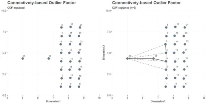
Inspecting the right plot in Figure 9, a set of nearest neighbors for observation 26 is identified with dashed line and is denoted as:

𝑁 (𝑝 ) = {5, 25, 4, 3, 6}

The 𝑆𝐵𝑁𝑝𝑎𝑡ℎ , ordering the observations in ascending order by distance to 𝑝 , is: 𝑆𝐵𝑁𝑝𝑎𝑡ℎ = {25, 4, 5, 3, 6}

The 𝑆𝐵𝑁𝑡𝑟𝑎𝑖𝑙 , identifying the shortest path for observations chaining distance, with solid line, is: 𝑆𝐵𝑁𝑡𝑟𝑎𝑖𝑙 = {(26, 25), (25, 4), (4, 3), (4, 5), (5, 6)}

The cost function, returning the distance from pairs in 𝑆𝐵𝑁𝑡𝑟𝑎𝑖𝑙 , is: 𝑐 = {1.7, 0.88, 1.08, 0.96, 0.97) The average chaining distance is then given by:

𝑎𝑐𝐷𝑖𝑠𝑡 = 2(5 + 1 − 1)

5(5 + 1) ∗ 1.7 +

2(5 + 1 − 2)

5(5 + 1) ∗ 0.88 + ⋯ = 6.07

28 𝐶𝑂𝐹 (𝑝 ) = 1.52

Figure 9: Dataset with observation 26 as outlier (left) and COF applied with k=5 (right)

Like INFLO and LOF, a COF of 1 indicates density – or isolativity – at the level of neighboring observations and COF greater than 1 indicates less dense neighborhood and outlierness. With the greatest COF, observation 26 ruled as the observation with the greatest outlierness. Again, as with LOF and INFLO, the disadvantage of COF is the subjectivety when choosing 𝑘.

For simplification, the LOF, COF and INFLO are described in one sentence:

 LOF identifies neighbors and express the ratio of distance between neighbors, and the neighboring observations of neighbors.

 COF identifies neighbors and express the ratio of distance between the most efficient chain for neighbors, and the most efficient chain for neighbors of neighbors.

 INFLO identifies reverse neighbors and express the ratio of distance between reverse neighbors, and the reverse neighboring observations of reverse neighbors.

For demonstration purposes of INFLO and COF, Figure 10 is created. The left plot shows few observations labelled with an outlierness ≥ 1.20, being the observations with greatest deviating characteristics. Three observations are identified as inliers between cluster in bottom left and the two outlying observations

29 assigned with an INFLO of 1.49 and 1.26. Returning to the idea of the reverse neighborhood, the three inlying observations identifies the two outlying observations as a part of their reverse neighborhood, explaining the low INFLO score. For comparison, right plot has the very same three observations assigned with a relatively high COF score, indicating outlierness. Thus, INFLO and COF has different ways of defining outlierness. In this particular case, the incoherence for assigned outlierness for the two algorithms is also a matter of setting the 𝑘 parameter right.

Figure 10: Comparison of INFLO (left) and COF (right) applied with k=10

3.2.7.4. Local Correlation Integral Method (LOCI)

Papadimitriou, Gibbons, & Faloutsos (2003) also adopted the density-based approach and criticized LOF for sensitivity when choosing 𝑘. It was argued that selecting a 𝑘 larger than cluster size of which an observation belongs to will create artificial high outlier-score. A small 𝑘 will on the other hand fail to identify small outlying clusters. Furthermore, the ‘magical cut-off point’ for the LOF-score to identify outliers was criticized. Papadimitriou, Gibbons, & Faloutsos (2003) proposed an algorithm, based on probabilistic reasoning, called Local Correlation Integral method (LOCI).

For probabilistic reasoning, a sample and counting neighborhood is introduced. For observation 𝑝 , the sample neighborhood is given by 𝑛(𝑝 , 𝑟), where 𝑟 is a radius. The counting neighborhood is given by 𝑛(𝑝 , 𝛼𝑟), where 𝛼 is number between 0 and 1, determining the size of the sampling neighborhood,

30 relatively to the counting neighborhood. 𝛼 = 0.5 is recommended to have a sampling neighborhood large enough to contain samples.

For each identified observation 𝑝 , within the sample neighborhood of observation 𝑝 , the set of neighbors is expressed as 𝑁(𝑝 , 𝑟) = {𝑝 ∈ 𝑛(𝑝 , 𝑟)|𝑑𝑖𝑠𝑡(𝑝 , 𝑝 ) ≤ 𝑟}. The count of neighbors in the set is expressed as |𝑁(𝑝 , 𝑟)|. For each member of 𝑁(𝑝 , 𝑟), a counting neighborhood is given by 𝑛(𝑝, 𝛼𝑟). The number of neighbors in 𝑛(𝑝, 𝛼𝑟) over the count of the sampling neighborhood is then given by:

𝑛(𝑝 , 𝑟, 𝛼) = ∑ ∈ ( , )𝑛(𝑝, 𝛼𝑟) |𝑁(𝑝 , 𝑟)|

The multi-granularity deviation factor, expressing the density of the counting neighborhood for observation 𝑝 relatively to the counting neighborhood for observation 𝑝 , is given by:

𝑀𝐷𝐸𝐹(𝑝 , 𝛼, 𝑟) = 1 −𝑛(𝑝 , 𝛼, 𝑟) 𝑛(𝑝 , 𝑟, 𝛼)

The counting neighborhood of observation 𝑝 , always contains 𝑝 . Thus, 𝑛(𝑝 , 𝑟, 𝛼) is always > 0. For the input parameter 𝑟, determining the size of both sampling and counting neighborhood, an 𝑟 large enough to identify 20 members of 𝑁(𝑝 , 𝑟) (|𝑁(𝑝 , 𝑟)| ≥ 20), was recommended as being enough to introduce statistical errors in 𝑀𝐷𝐸𝐹 and 𝜎𝑀𝐷𝐸𝐹.

To avoid the ‘magical cut-off point’, a normalized standard deviation of the counting neighborhood 𝑛(𝑝 , 𝑟, 𝛼) was introduced, given by:

𝜎𝑀𝐷𝐸𝐹(𝑝 , 𝛼, 𝑟) =𝜎𝑛(𝑝 , 𝑟, 𝛼) 𝑛(𝑝 , 𝑟, 𝛼)

If MDEF is sufficiently large, an observation is labelled as an outlier given by: 𝑀𝐷𝐸𝐹(𝑝 , 𝛼, 𝑟) > 𝑘 𝜎𝑀𝐷𝐸𝐹(𝑝 , 𝛼, 𝑟)

where 𝑘 = 3 is recommended as less than 1% of the observations in a normal distribution are beyond the .999 confidence interval.

Inspecting the left plot in Figure 11, a sampling neighborhood 𝑛(𝑝 , 𝑟) for observation 𝑝 is given by 𝑟 = 2.25. The counting neighborhood is given by 𝛼 = 0.4, or 40% of sampling neighborhood. Within the sample neighborhood of observation 𝑝 , a set of neighbors are identified, 𝑁(𝑝 , 𝑟) = {𝑝 , 𝑝 , 𝑝 , 𝑝 }. For

31 𝑛(𝑝 , 𝛼𝑟) and 𝑛(𝑝 , 𝛼𝑟) 7 and 5 observations are identified, respectively. 𝑛(𝑝 , 𝛼𝑟) and 𝑛(𝑝 , 𝛼𝑟) both have 1 observation in their counting neighborhood, hence 𝑛(𝑝 , 𝑟, 𝛼) = (1+7+5+1)/4 = 3.5.

Figure 11: LOCI theory illustrated (left) and applied on synthetic data (right)

The multi-granularity deviation factor for observation 𝑝 is then:

𝑀𝐷𝐸𝐹(𝑝 , 𝛼, 𝑟) = 1 −𝑛(𝑝 , 𝛼, 𝑟)

𝑛(𝑝 , 𝑟, 𝛼)= 1 −

1

3.5= 0.71

Meaning that observation 𝑝 has a less dense counting neighborhood than 𝑝 , 𝑝 and 𝑝 . The standard deviation for 𝑛(𝑝 , 𝑟, 𝛼) is given by:

𝜎𝑛(𝑝 , 𝑟, 𝛼) = ∑ 𝑛(𝑝, 𝛼𝑟) − 𝑛(𝑝 , 𝑟, 𝛼)

|𝑁(𝑝_𝑖, 𝑟)|− 1 = 3

And the normalized standard deviation is given by:

𝜎𝑀𝐷𝐸𝐹(𝑝 , 𝛼, 𝑟) =𝜎𝑛(𝑝 , 𝑟, 𝛼)

𝑛(𝑝 , 𝑟, 𝛼) =

3

3.5= 0.85

Thus, following the rule of a sufficiently larger MDEF with 𝑘 = 3, observation 𝑝 is not labelled as an outlier.