Voestalpine AG : equity valuation

Executive Summary

Voestalpine AG is a steel-based technology and capital goods group and a world leader in the manufacture, processing, and development of sophisticated steel products. The Group supplies technology-intensive sectors, such as the automotive, railway, aviation, and energy industries.

The Group had adopted the development strategy for the decade, targeting 2 billion EUR in total revenue by 2020, which is 73% higher compared to the most recent result. The strategy also implies the steady investments of 800 – 1000 million EUR per year.

The reports considers all the public information provided by the Voestalpine Group, careful investigation of global economic prospects and separate study of each of the industries operated by the Group.

The main valuation was done by means of Enterprise Discounted Cash Flow model, which was chosen as the most appropriate approach assuming all the inputs. By taking into consideration the possible scenarios of economic and market development, the target price was accompanied with VAR and extended range for target price.

The thesis target price is compared to the report provided by JP Morgan. Even though the results do not match, the difference is moderate.

Recommendation

BUY

Thesis target price

38,23 EUR

JP Morgan fair price

40 EUR

Favorable market conditions

46,15 EUR

Voestalpine AG

Acknowledgement

I would like to express my gratitude to Professor José Carlos Tudela Martins for his constant availability and valuable contribution; to the analysts Rui Dias and Ulugbek Suyumov from BESI for all the information provided; to my colleagues from the Dissertation Seminars for all the positive and productive discussions, and finally to my family for all the support given.

Table of Content

Executive Summary ... 1

Acknowledgement ... 2

List of Abbreviations ... 5

Introduction ... 7

Valuation Approaches Overview ... 7

Discounted Cash Flow ... 8

Adjusted Present Value ... 9

Dividend Discount Model (DDM) ... 11

Enterprise Discounted Cash flow ... 11

Free Cash flow to the Equity ... 13

Terminal Value ... 13

Economic-Profit Based Valuation ... 14

Cost of Financing ... 15

Relative Valuation ... 17

Contingent Claim Valuation ... 19

Conclusion ... 20

Company Overview ... 21

Steel Division ... 25

Special Steel Division ... 26

Metal Engineering Division ... 27

Metal Forming Division ... 28

Industry Overview ... 29

Cost of Capital ... 32

Cost of Debt ... 32

Cost of Equity ... 34

Weighted Average Cost of Capital ... 35

Revenue Projections... 36

Scenario 1 (Estimated growth rates) ... 36

Scenario 2 (“Strategy 2020”) ... 37

Cost of Goods Sold ... 37

Operating Revenue and Operating Expenses ... 38

Depreciation and CAPEX ... 39

Working Capital ... 41

Enterprise Discounted Cash Flow ... 44

Relative Valuation ... 45

Dividend Discount Model ... 48

Valuation Comparison: Models ... 49

Sensitivity Analyses ... 49

Value at Risk ... 51

Valuation Comparison: JP Morgan ... 52

Bibliography ... 53

Appendix ... 55

Growth rate projections ... 55

Projections by Divisions... 60

Working Capital ... 62

Interest Expenses ... 63

Sensitivity Analyses ... 65

List of Abbreviations

AD – accumulated depreciation

AP –account payables

APV – adjusted present value

AR – account receivables

BV – book value βl – beta levered

βu – beta unlevered

CAGR – compounded annual growth rate

CAPEX – capital expenditures

CAPM – capital asset pricing model

D – market value of debt

DCF – discounted cash flow

DDM – dividend discount model

DPS – dividends per share

E – market value of equity

EBIT – earnings before interest and taxes

EBITDA – earnings before interest taxes depreciation and amortization

EDCF – enterprise discounted cash flow

EV – enterprise value

EVA – economic value added

EVM – enterprise value multiples

FCFE – free cash flow to the equity

g – growth rate

Kd – cost of debt

Ke – cost of equity

Ku – cost of equity unlevered

MV – market value

MVA – market value added

NOPLAT – net operating profit less adjusted taxes

PE – price earning

PPE – property plant equipment

Rf – risk free rate

ROE – return on equity

ROIC – return on invested capital

tc – tax rate

VAR – value at risk

WA – weighted average

WACC – weighted average cost of capital

Introduction

One the main objectives’ of any country is the achieving economic growth. For this reason a lot of efforts are dedicated for the development of all sized enterprises, as they are drivers of economy. So, financing and stimulating the evolvement of local businesses is the priority for the state. At the same time, not only the government is interested in financially successful projects. The investors, who exchange their current assets for the future dividends, may be faced to even a greater risk, comparing to else ones. However, by bearing more uncertainty of the projects, the shareholders are expected to receive higher interests. Hence, by the statements above it can be concluded that the investments are made with the intention of receiving future paybacks in terms of higher capacity performance and employment rate for the country and higher dividends for the investors.

According to Tim Koller (2010): “Companies create value for their owners by investing cash now to generate more cash in the future. The amount of value they create is the difference between cash inflows and the cost of the investments made, adjusted to reflect tomorrow’s cash flows are worth less than today’s because of the time value of money and riskiness of future cash flows”. Therefore, the primary task for the investors is determining the value of the project. However, there is no a straightforward and universal approach, which would let the shareholders to calculate precise amount of future dividends. As Damodaran (2002) states: “Every asset, financial as well as real, has a value. The key to successfully investing in and managing these assets lies in understanding not only what the value is, but also the sources of the value. Any asset can be valued, but some assets are easier to value than others and the details of valuation will vary from case to case”. Thus, the assessment of the project must consider variety of specific inputs of the business, which include all the risks and data anyhow influencing the final result. For these reasons, different approaches of valuation were developed, suiting the specifications of diversity of cases. The following literature review is dedicated for the study of valuation approaches most suitable for Voestalpine AG.

Valuation Approaches Overview

As it was stated in the previous paragraph there is a wide range of models used for valuing the company. Even though, the approaches often required different data and assumptions, they share some common characteristics in broader terms. In general, there are four approaches of valuation. (Damodaran, 2006) The first, discounted cash flow valuation, derives the value of the asset through the sum of present value of future cash flows projected by this asset. The second, liquidation and accounting valuation, considers the net amount that can be realized by selling assets of a firm and paying off the debt. The third, relative valuation, estimates the value of an asset by looking at the value of similar asset in the market. The final approach, contingent claim valuation, uses option pricing models to measure the value of assets that share option characteristics. (Damodaran, 2006)

Discounted Cash Flow

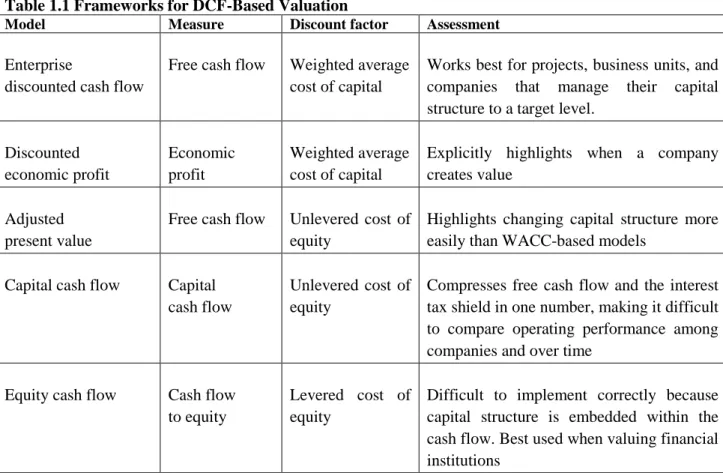
The discounted cash flow (DCF) valuation is based on the concept of the present value rule, considering the value of any asset as its expected future cash flows discounted to the present date. As it can be clearly seen from the definition of DCF, there are two main stages required to accomplish this method. The first one is determining all the expected cash flows and the second step is applying the proper discount rate. Even though there are only two dimensions to maneuver in this approach, there are hundreds of ways of calculating future inflows of capital, by grouping them to categories and matching them for different discount and growth rates. Moreover, the existence of variety of sources for financing needs, assuming both domestic and international ones, and the presence of mixed capital structures in the companies, creates for the process of estimation the proper discount rate diverse methods. As the result, there are thousands of DCF models available for application. However, Damodaran (2002) offers three main dimensions for using this model, which are estimating equity value, firm value and adjusted present value. At the same time, some of the models might be called in a different way, while presenting the same concepts. For instance, free cash flow to the firm (FCFF) can also be called enterprise discounted cash flow (EDCF). In the exhibit below, the framework for DCF-Based Valuation is presented.

Table 1.1 Frameworks for DCF-Based Valuation

Model Measure Discount factor Assessment

Enterprise

discounted cash flow

Free cash flow Weighted average cost of capital

Works best for projects, business units, and companies that manage their capital structure to a target level.

Discounted economic profit Economic profit Weighted average cost of capital

Explicitly highlights when a company creates value

Adjusted present value

Free cash flow Unlevered cost of equity

Highlights changing capital structure more easily than WACC-based models

Capital cash flow Capital cash flow

Unlevered cost of equity

Compresses free cash flow and the interest tax shield in one number, making it difficult to compare operating performance among companies and over time

Equity cash flow Cash flow to equity

Levered cost of equity

Difficult to implement correctly because capital structure is embedded within the cash flow. Best used when valuing financial institutions

Adjusted Present Value

In most of the DCF models the analysts assume WACC in valuations. However, this approach considers a constant debt-to-value ratio, which is a controversial assumption. As firm’s debt may increase in the same paste as the overall growth of the company, the use of WACC is considered as reasonable. At the same time, changes in capital structure, for instance, the decrease of debt-to-value ratio with the improved cash flows, will result in meaningless values – overstating tax shield. Therefore, the alternative model of valuation, separating the value of operations into two components, which are the value of operations as if the company were all-equity financed and the value of the tax shield that arises from debt financing, was introduced. The model is called adjusted present value (APV). (Koller, 2010)

Another famous critique work for using APV instead of WACC models belongs to T. Luehrman (1997) called “Using APV: A better tool for valuing operations”. In this article the author states the obsoleteness of WACC, due to poor ability of the method to handle financial side effects. Meanwhile, “APV’s approach is to analyze financial maneuvers separately and then add their value to that of the business”. (Luehrman, 1997) Thus, dividing the valuation into parts provide management more informative results, as it makes it possible to observe all the components of the value in the analysis. The fundamental idea of APV is presented in the illustration below by T.Luerhman. (1997)

Illustration 1.1 APV Fundamental Idea

+

Value of financing side effects Base-case value

interest tax shields

APV

=

Value of the project as if it were financed entirely with equity

costs of financial distress Subsidies

Hedges issues costs other costs

Meanwhile, Damodaran (2002) proposes the three stage procedure to calculate APV. The first one requires the estimation of the value of the firm with no leverage. Secondly, the present value of interest tax savings resulted from borrowings must be calculated. Finally, the probability and expected cost of bankruptcy should be evaluated.

To accomplish the first step, the expected free cash flow to the firm must be discounted by the unlevered cost of equity. For the case of constant growth rate in perpetuity, the following formula is presented.

𝑉𝒂𝒍𝒖𝒆 𝒐𝒇 𝑼𝒏𝒍𝒆𝒗𝒆𝒓𝒆𝒅 𝑭𝒊𝒓𝒎 = 𝑭𝑪𝑭𝑭𝟎(𝟏 + 𝒈) 𝒌𝒖− 𝒈

With the purpose of calculating the unlevered cost of equity, the CAPM is used along with the unlevered Beta, which is derived as:

𝜷𝒖𝒏𝒍𝒆𝒗𝒆𝒓𝒆𝒅 = 𝜷𝒄𝒖𝒓𝒓𝒆𝒏𝒕 𝟏 + (𝟏 − 𝒕)𝑫_𝑬

The second step in valuation of APV is calculating the expected tax benefits of financing side effects. According to Damodaran (2002) tax benefits should be discounted at the cost of debt to reflect the riskiness of this cash flow. However, Koller (2010) suggests the unlevered cost of capital is more appropriate for valuation, as there is always a possibility that the company will not be able to fully use the tax shield, due to low profits. Thus, tax shield may be discounted by both ways, as there is still no unambiguous opinion among analyst.

= (𝑻𝒂𝒙 𝑹𝒂𝒕𝒆)(𝑪𝒐𝒔𝒕 𝒐𝒇 𝑫𝒆𝒃𝒕)(𝑫𝒆𝒃𝒕) 𝑪𝒐𝒔𝒕 𝒐𝒇 𝑫𝒆𝒃𝒕

𝑽𝒂𝒍𝒖𝒆 𝒐𝒇 𝑻𝒂𝒙 𝑩𝒆𝒏𝒆𝒇𝒊𝒕𝒔 = (𝑻𝒂𝒙 𝑹𝒂𝒕𝒆)(𝑫𝒆𝒃𝒕)

= 𝒕𝒄𝑫

Finally, the negative side of carrying debt is to be estimated for APV. By borrowing assets, the company obliges itself for future cash outflows in terms of interest and principle repayments. However, the inability of the firm to satisfy its contractual commitments to the second party may result in bankruptcy. There are two sources of bankruptcy cost: direct and indirect. If calculation of direct bankruptcy cost, which include legal and administrative cost, straightforward, the estimation of indirect one is more complex. The indirect cost comprises of losing customers, stricter terms from suppliers and difficulties in raising new capital. As the result of complication of valuating bankruptcy cost, this step is considered as main disadvantages of APV model. Moreover, it is required to determine the probability of bankruptcy, which is also a complex process. However, Altman and Kishore (1998) related the bond ratings to the probability of default rate, making it easier to estimate expected bankruptcy cost.

𝑷𝑽 𝒐𝒇 𝑬𝒙𝒑𝒆𝒄𝒕𝒆𝒅 𝑩𝒂𝒏𝒌𝒓𝒖𝒑𝒕𝒄𝒚 𝒄𝒐𝒔𝒕 =₌ (𝑷𝒓𝒐𝒃𝒂𝒃𝒊𝒍𝒊𝒕𝒚 𝒐𝒇 𝑩𝒂𝒏𝒌𝒓𝒖𝒑𝒕𝒄𝒚)(𝑷𝑽 𝒐𝒇 𝑩𝒂𝒏𝒌𝒓𝒖𝒑𝒕𝒄𝒚 𝑪𝒐𝒔𝒕)

𝝅𝑩𝑪

All in all, APV relies on value additivity, which is breaking the project into pieces and allowing managers to get more specific information about where the value comes from. Meanwhile, WACC is considered suitable only for simples and most static of capital structures. However, the drawbacks of APV is determining the right discount rate for the tax shields, estimating the probability and the indirect cost of bankruptcy. All these factors make this model of valuation complex and difficult to apply.

Dividend Discount Model (DDM)

A value of the bond at a given point in time can be defined as the present value of the stream of coupon payments plus principal payment to be received at maturity, both discounted at the prevailing rate of interest for that maturity. Assuming the analogous reasoning, the value of a common stock can be defined as the present value of the future dividend stream in perpetuity. This concept is consistent with the assumption that the corporation will indeed have a perpetual life, in accordance with its charter. (Farrel J., 1985) As the result the following formula can be derived.

𝑽𝒂𝒍𝒖𝒆 𝒐𝒇 𝒔𝒕𝒐𝒄𝒌 = ∑ 𝑬(𝑫𝑷𝑺𝒕) (𝟏 + 𝒌𝒆)𝒕 𝒕= ∞

𝒕=𝟏

Assuming the stable growth rate in dividends for infinite timeframe, the Gordon Growth Model can be used to value firms stock. So,

𝑽𝒂𝒍𝒖𝒆 𝒐𝒇 𝒔𝒕𝒐𝒄𝒌 = 𝑫𝑷𝑺𝟏 𝒌_𝒆− 𝒈

However, the approach is limited to firms that are growing at a stable rate. The Gordon growth model is extremely sensitive to the inputs for the growth rate. Since the growth rate in the firm’s dividends is expected to last forever, the firms other measures of performance can also be expected to grow at the same rate. Also, dividend policy can be manipulated by the management, in order to create an illusion of a growing company. Meanwhile, distributing most of the earnings to investors may lead to a lower plowback ratio, resulting in a slower or no growth of the firm. Therefore, using the DDM requires detailed study of dividends policy of the company and future prospects, and determining whether company is creating value or just distributing it all to investors. (Damodaran, 2002)

Enterprise Discounted Cash flow

As Koller (2010) states : “The enterprise DCF model discounts free cash flow, meaning the cash flow available to all investors—equity holders, debt holders, and any other nonequity investors—at the weighted average cost of capital, meaning the blended cost for all investor capital.” Damodaran (2002) suggest two ways for calculating the cash flow to the firm.

FCFF = Free Cash flow to Equity + Interest Expense (1 – tax rate) + Principal Repayments – New Debt Issues + Preferred Dividends

FCFF = EBIT (1 – tax rate) + Depreciation – Capital Expenditure – ∆ Working Capital

The term of EBIT*(1-t) is also referred as net operating profit less adjusted taxes (NOPLAT).Thus, after determining the FCFF it is required to calculated weighted average cost of capital (WACC). As the FCFF are available for all investors, so the discount rate should represent the risks faced by all of the parties.

Thus, WACC mixes the rates of return required by debt and equity holders. According to the famous capital structure irrelevance proposition by Modigliani and Miller (1958), which assumes the world without taxes, transaction costs, no bankruptcy cost and symmetry of market information, there is no impact of debt on value of the company. In other words, the capital structure of the company would not influence the WACC, as there is no interest tax shield, and it would stay constant. However, the assumptions of the theorem are not present in reality, therefore the calculation of WACC should assume the side effects of debt. Hence, WACC is estimated as follows:

𝑾𝑨𝑪𝑪 = 𝑫

𝑫 + 𝑬𝒌𝒅(𝟏 − 𝑻) + 𝑬 𝑫 + 𝑬𝒌𝒆

The general formula for FCFF model is presented as the sum of expected free cash flows discounted by WACC. However, analyst usually prefer dividing the analyses into two parts, which are forecasting the value of the firm for the explicit forecast period and adding up the value of the company after the explicit period. The intuition upon this concept is that most of the companies reach a stable growth period in their lifecycle, therefore it is assumed that the company is going to expand on the same rate in perpetuity. Moreover, predicting the performance of the company at some point becomes impractical and very subjective. As the result infinite constant growth is assumed. Thus, the following formula is proposed by Damodaran (2002): 𝑽𝒂𝒍𝒖𝒆 𝒐𝒇 𝑭𝒊𝒓𝒎 = ∑ 𝑭𝑪𝑭𝑭𝒕 (𝟏 + 𝑾𝑨𝑪𝑪)𝒕+ [𝑭𝑪𝑭𝑭_𝒏+𝟏/(𝑾𝑨𝑪𝑪 − 𝒈_𝒏)] (𝟏 + 𝑾𝑨𝑪𝑪)𝒏 𝒕=𝒏 𝒕=𝟏

On the other hand, Koller (2010) suggest the application of alternative way for estimating continuing value. In his formula, the cash flow is directly linked to growth and ROIC.

𝑪𝒐𝒏𝒕𝒊𝒏𝒖𝒊𝒏𝒈 𝑽𝒂𝒍𝒖𝒆𝒕 = 𝑵𝑶𝑷𝑳𝑨𝑻𝒕 + 𝟏(𝟏 − 𝒈 𝑹𝑶𝑰𝑪) 𝑾𝑨𝑪𝑪 − 𝒈

The limitation of the enterprise discounted cash flow approach is the heavy dependence on WACC which assumes constant capital structure for the companies. However, as contemporary studies display the capital structure is highly correlated with the life cycle of the company, therefore tends to change periodically.(La Rocca, 2011) Moreover, the WACC is significantly lower than cost of equity for most of the cases, which increases the value of the company. Finally, the model is vulnerable against the assumption related to CAPEX and depreciation. The reinvestment needs must be directly connected to the expected growth of the company, otherwise FCFF can be manipulated easily.

Free Cash flow to the Equity

The equity cash flow model values equity directly by discounting cash flows to equity at the cost of equity, unlike free cash flow to the firm models. To calculate the cash flow available for shareholders the following algorithm is used:

Free Cash Flow to Equity = Net Income – (Capital Expenditures – Depreciation) – (Change in Non-cash Working Capital) + (New Debt Issued – Debt Repayments)

FCFE does not have significant difference with the dividends discount model. The only assumption is that FCFE will be totally distributed to the shareholders, while in DDM the actual dividends are considered. (Damodaran, 2002). Thus, if the constant growth rate is assumed, the formula of calculating value of stock of the company is similar to the Gordon growth model.

𝑽𝒂𝒍𝒖𝒆 𝒐𝒇 𝒔𝒕𝒐𝒄𝒌 = 𝑭𝑪𝑭𝑬 𝒌_𝒆− 𝒈

If the expected growth rate is estimated by the standard approach, product of retention ratio by return on equity, it will not be consistent with the general assumption of the model that all FCFE is paid out to stockholders. However, as the reinvestments are required to sustain growth of the company, the adjustments should be made. As Damodaran (2002), states: “It is more consistent to replace the retention ratio with the equity reinvestment rate, which is measures the percent of net income back into firm”.

𝑬𝒒𝒖𝒊𝒕𝒚 𝑹𝒆𝒊𝒏𝒗𝒆𝒔𝒕𝒎𝒆𝒏𝒕 𝑹𝒂𝒕𝒆 = 𝟏 − 𝑵𝒆𝒕 𝑪𝑨𝑷𝑬𝑿 + 𝑪𝒉𝒂𝒏𝒈𝒆 𝑰𝒏 𝑾𝒐𝒓𝒌𝒊𝒏𝒈 𝑪𝒂𝒑𝒊𝒕𝒂𝒍 − 𝑵𝒆𝒕 𝑫𝒆𝒃𝒕 𝑰𝒔𝒔𝒖𝒆𝒔 𝑵𝒆𝒕 𝑰𝒏𝒄𝒐𝒎𝒆

The ROE should also be modified as it includes returns from excess cash and marketable securities, while FCFE model does not have excess cash left.

𝑵𝒐𝒏 − 𝒄𝒂𝒔𝒉 𝑹𝑶𝑬 = 𝑵𝒆𝒕 𝑰𝒏𝒄𝒐𝒎𝒆 − 𝑨𝒇𝒕𝒆𝒓 𝒕𝒂𝒙 𝒊𝒏𝒄𝒐𝒎𝒆 𝒇𝒓𝒐𝒎 𝒄𝒂𝒔𝒉 𝒂𝒏𝒅 𝒎𝒂𝒓𝒌𝒆𝒕𝒂𝒃𝒍𝒆 𝒔𝒆𝒄𝒖𝒓𝒊𝒕𝒊𝒆𝒔 𝑩𝒐𝒐𝒌 𝑽𝒂𝒍𝒖𝒆 𝒐𝒇 𝑬𝒒𝒖𝒊𝒕𝒚 − 𝑪𝒂𝒔𝒉 𝒂𝒏𝒅 𝑴𝒂𝒓𝒌𝒆𝒕𝒂𝒃𝒍𝒆 𝑺𝒆𝒄𝒖𝒓𝒊𝒕𝒊𝒆𝒔

Finally, to derive the growth rate the above stated rates should be multiplied. Expected Growth in FCFE = Equity Reinvestment Rate * Non – cash ROE

The model is best for firms growing at a rate comparable to or lower than nominal growth in economy. The FCFE model can vary in the same directions as FCFF does, assuming constant growth, two-stage model, three -two-stage model and so on.

Terminal Value

The intuition behind this model lies on the assumption that in the long-term prospective, firm’s growth rate is tend to converge with the growth of economy. For this reason, the value of the company at some point of time is considered to grow in perpetuity. As the result one of the approaches of calculating the

terminal value of the firm is simply discounting cash flow from the next period by the difference of cost of capital and the growth rate.

𝑻𝒆𝒓𝒎𝒊𝒏𝒂𝒍 𝒗𝒂𝒍𝒖𝒆 𝒐𝒇 𝑬𝒒𝒖𝒊𝒕𝒚_𝒏= 𝑪𝒂𝒔𝒉 𝒇𝒍𝒐𝒘 𝒕𝒐 𝑬𝒒𝒖𝒊𝒕𝒚 𝑪𝒐𝒔𝒕 𝒐𝒇 𝑬𝒒𝒖𝒊𝒕𝒚_𝒏+𝟏− 𝒈

𝑻𝒆𝒓𝒎𝒊𝒏𝒂𝒍 𝒗𝒂𝒍𝒖𝒆_𝒏= 𝑪𝒂𝒔𝒉 𝒇𝒍𝒐𝒘 𝒕𝒐 𝑭𝒊𝒓𝒎 𝑪𝒐𝒔𝒕 𝒐𝒇 𝑪𝒂𝒑𝒊𝒕𝒂𝒍_𝒏+𝟏− 𝒈

However, if the return on capital is equal to the stable growth rate, increasing growth rate will not have impact of value (Damodaran, 2002).

𝑻𝒆𝒓𝒎𝒊𝒏𝒂𝒍 𝑽𝒂𝒍𝒖𝒆_{𝑹𝑶𝑪=𝑾𝑨𝑪𝑪}= 𝑬𝑩𝑰𝑻𝒏+𝟏(𝟏 − 𝒕) 𝑪𝒐𝒔𝒕 𝒐𝒇 𝑪𝒂𝒑𝒊𝒕𝒂𝒍_𝒏

The alternative approach of estimating the terminal value is related to the assumption that all the existing assets are going to be sold in the future. This model is referred as liquidation value. Expected Liquidation value equals to the book value of assets multiplied by one plus inflation rate in the power of average years of the assets. This concept is different from the going concern, as it is not expected that the company will operate infinitely. The effect of this approach depends on the performance of the industry, for growing ones it will result in a lower value comparing to going concern, and in vanishing industry it will have better values. (Koller, 2010)

Economic-Profit Based Valuation

“Economic Value Added is a value based measure that gives the importance on value creation by the management for the owners. It comes closer than any other capturing the true economic profit for enterprise”. (Shil, 2009) EVA assists analyst to determine the source of the value creation as long as the time when it was observed. This type of model measures the dollar surplus value added by an investment. The computation of the EVA is straightforward and very logical. It is estimated by the product of invested capital with the difference of return on invested capital (ROIC) and the cost of capital (WACC). Thus, it may seem that EVA is actually a residual income (RI). Nevertheless, EVA handles accounting distortions, by using up to 164 adjustments to traditional accounting data (Stewart, 1991; Blair, 1997).

In 1990, Stewart has defined the following formula: 𝐸𝑉𝐴 = 𝑁𝑂𝑃𝐿𝐴𝑇 – 𝐶𝑎𝑝𝑖𝑡𝑎𝑙 𝐶𝑜𝑠𝑡 𝑁𝑂𝑃 (1 − 𝑇) – 𝐶𝑎𝑝𝑖𝑡𝑎𝑙 𝐸𝑚𝑝𝑙𝑜𝑦𝑒𝑑 ∗ 𝐶𝑜𝑠𝑡 𝑜𝑓 𝐶𝑎𝑝𝑖𝑡𝑎𝑙 𝐴𝑑𝑗𝑢𝑠𝑡𝑒𝑑 𝑁𝑂𝑃 (1 – 𝑇) – 𝐶𝑎𝑝𝑖𝑡𝑎𝑙 𝐸𝑚𝑝𝑙𝑜𝑦𝑒𝑑 ∗ 𝑊𝐴𝐶𝐶 𝐴𝑑𝑗𝑢𝑠𝑡𝑒𝑑 𝑁𝑂𝑃 (1 – 𝑇) − [𝐶𝑎𝑝𝑖𝑡𝑎𝑙 𝐸𝑚𝑝𝑙𝑜𝑦𝑒𝑑 {(𝐾𝑒 𝐸 𝐶𝐸) + (𝐾𝑑 𝐷 𝐶𝐸) (1 − 𝑇) + … . }] 𝑅𝑒𝑡𝑢𝑟𝑛 – 𝐶𝑎𝑝𝑖𝑡𝑎𝑙 𝐸𝑚𝑝𝑙𝑜𝑦𝑒𝑑 ∗ 𝑊𝐴𝐶𝐶 (𝑅𝑎𝑡𝑒 𝑜𝑓 𝑅𝑂𝐼 – 𝑊𝐴𝐶𝐶) 𝐶𝑎𝑝𝑖𝑡𝑎𝑙 𝐸𝑚𝑝𝑙𝑜𝑦𝑒𝑑

Also, for the listing companies the calculation of EVA via market value added was proposed: 𝑀𝑉𝐴 = 𝑀𝑎𝑟𝑘𝑒𝑡 𝑉𝑎𝑙𝑢𝑒 𝑜𝑓 𝑡ℎ𝑒 𝐶𝑜𝑚𝑝𝑎𝑛𝑦 − 𝐶𝑎𝑝𝑖𝑡𝑎𝑙 𝐼𝑛𝑣𝑒𝑠𝑡𝑒𝑑 𝑀𝑎𝑟𝑘𝑒𝑡 𝑉𝑎𝑙𝑢𝑒 𝑜𝑓 𝐸𝑞𝑢𝑖𝑡𝑦 − 𝐵𝑜𝑜𝑘 𝑉𝑎𝑙𝑢𝑒 𝑜𝑓 𝐸𝑞𝑢𝑖𝑡𝑦 (𝑀𝑉 − 𝐵𝑉) 𝑛𝑢𝑚𝑏𝑒𝑟 𝑜𝑓 𝑠ℎ𝑎𝑟𝑒𝑠 𝑜𝑢𝑡𝑠𝑡𝑎𝑚𝑛𝑑𝑖𝑛𝑔 𝑃𝑟𝑒𝑠𝑒𝑛𝑡 𝑉𝑎𝑙𝑢𝑒 𝑜𝑓 𝐴𝑙𝑙 𝐹𝑢𝑡𝑢𝑟𝑒 𝐸𝑉𝐴 𝑀𝑎𝑟𝑘𝑒𝑡 𝑉𝑎𝑙𝑢𝑒 𝑜𝑓 𝐸𝑞𝑢𝑖𝑡𝑦 = 𝐵𝑜𝑜𝑘 𝑉𝑎𝑙𝑢𝑒 𝑜𝑓 𝐸𝑞𝑢𝑖𝑡𝑦 + 𝑃𝑟𝑒𝑠𝑒𝑛𝑡 𝑉𝑎𝑙𝑢𝑒 𝑜𝑓 𝐴𝑙𝑙 𝐹𝑢𝑡𝑢𝑟𝑒 𝐸𝑉𝐴

The similarity of MVA to market-to-book ratio is obvious. However, MVA presents absolute measure, while MBR a relative one. (Shil, 2009) Thus, in order to find the value of the company considering EVA, the invested capital should be summed up with the present value of excess returns on these investments. (Koller, 2010) 𝑽𝒂𝒍𝒖𝒆𝟎= 𝑰𝒏𝒗𝒆𝒔𝒕𝒆𝒅 𝑪𝒂𝒑𝒊𝒕𝒂𝒍𝟎+ ∑ 𝑰𝒏𝒗𝒆𝒔𝒕𝒆𝒅 𝑪𝒂𝒑𝒊𝒕𝒂𝒍_𝒕−𝟏× (𝑹𝑶𝑰𝑪_𝒕− 𝑾𝑨𝑪𝑪) (𝟏 + 𝑾𝑨𝑪𝑪)𝒕 ∞ 𝒕=𝟏

As it can be seen from the formula, in the case of absence of future economic profit, the value of the company would equal to the invested capital. Also, the formula allows analyst to determine expectations regarding future value creation. Meanwhile, comparing to FCFF model, which could keep growing even facing a decrease in ROIC, EVA manages this issue. Among the other advantages of this model, the strong relationship of EVA to share prices was identified by Stewart in 1990.

On the hand, there are some limitations, deteriorating the application of this model. First of all, EVA is more focused on short-term performance, therefore companies oriented in long-term investments usually fail to apply it. Secondly, it is not the best model for start-ups. The high investments of such companies in the current period are expected to receive positive cash flows only in a distant future, as a result making EVA less attractive. Finally, comparing to traditional ratios, EVA does not have any incremental value in predictions. (Shil, 2009)

Cost of Financing

By investing capital to the projects shareholders are expecting to receive returns excess to their investment. The present value of the investment is linked to the future one by the discount rate which represents the interest of investors and is referred as cost of equity. The most widespread model used for calculation of is called capital asset pricing model (CAPM). The model was developed by Treynor, Sharpe, Lintner and Mossin in early 1960s, and further refined later. The model predicts the relationship between the risk and equilibrium expected returns on risky assets (Bodie, 2004).

The model has a number of simplifying assumptions, having a fundamental idea that all of the investors are as similar as possible. The assumptions lead to the idea of equilibrium in hypothetical world of

securities and investors. As a result, the following implications can be elaborated. Firstly, all investors will chose to hold the market portfolio. Secondly, the market portfolio will be on the efficient frontier, representing the optimal risky portfolio. The concept was introduced by Markowitz in 1952. Thirdly, the risk premium on market portfolio is proportional to the variance of the market portfolio and investors degree of risk aversion (Bodie, 2004). Finally, the risk premium on individual asset will be proportional to the risk premium on the market portfolio and to the beta coefficient of the security on the market portfolio. Thus, CAPM suggests that the cost of equity is equal to the return on risk-free security plus a company’s systematic risk, multiplied by a market risk premium (Copeland, 1996).

E(Ri)= Rf +𝛃𝐢[E(Rm)- Rf]

E(Ri) - Expected Retur on Equity Rf – Risk-free rate

𝛃𝐢 – relationship between market risk of equity and the risk of market

E(Rm) – expected market return

Although, the model is one of the postulates in the contemporary financial world, it does not provide the comprehensive information about its application. For instance, each of the factors in the formula can be assumed or calculated by investors in different manners. The issue of which of the rates should be used as a risk-free or risk-premium and the source of Beta is not determined by the concept creators.

At least the absolute majority of analyst agrees that for the source of risk-free rate government default-free bonds should be considered. By the nature of contemporary business and financial world there is no entity possible to eliminate the default risk down to zero. Even being the representative of the most developed economy or being the most financially stable company for decades, does not assure the ability to fulfill contractual obligations. Damodaran (2012) suggest that the control of the printing of currency by the government, allows the country to always fulfill their promises at least in nominal terms.

The model of using government default-free bonds for risk-free rate arises the issue of selecting the right maturity, as they generate different yields. The ideal valuation is when each of the cash flow is discounted by the government bond with the same maturity. However, for the simplicity most applicable is a single yield to maturity 10-years government zero coupon bond.

Meanwhile, estimating the market risk premium is one of the most debated issue in finance. There are three main approaches of defining the market risk premium. The first one is using the historical data and use it as a proxy for future returns. The second method is running regression models linking different ratios to the expected risk premium. Finally, using the reverse engineer in DCF models to reach market’s cost of capital. The below approach is offered by Koller (2010)

𝒌𝒆 = 𝑬𝒂𝒓𝒏𝒊𝒏𝒈𝒔 (𝟏 − 𝒈 𝑹𝑶𝑬)

Regarding the determination of Beta, there are also several approaches available to do it. The most common one is using regression model, which regresses the historical returns of the company against market index ones (Damodaran, 2002).The estimation of the raw Beta is mostly done by regressing the market model:

𝑹𝒊 = 𝒂 + 𝜷𝑹𝒎 + 𝜺

As the model results in raw Beta, it is required to derive an unlevered industry Beta and then relevering Beta to the company’s target capital structure, this will improve the results of regression (Koller,2010). Fernandez (2004) assumes that the relationship of the levered and unlevered Beta is:

𝜷𝒍 = 𝜷𝒖 + (𝜷𝒖 − 𝜷𝒅) (𝑫

𝑬) (𝟏 − 𝑻)

To summarize the proper steps to be taken for the accomplishment of CAPM, Koller (2010) proposes the following considerations: “To estimate the risk-free rate in developed economies, use highly liquid, long-term government securities, such as the 10-year zero-coupon STRIPS. Based on historical averages and forward-looking estimates, the appropriate market risk premium is between 4.5 and 5.5 percent. To estimate a company’s beta, use an industry-derived unlevered beta relevered to the company’s target capital structure. Company-specific betas vary too widely over time to be used reliably”.

Relative Valuation

Even though DCF models tend to appeal most of the investors’ attention, in reality relative valuations are the most applied. In relative valuation, the price of the asset is estimated through the comparison to the value of the similar asset in the market. In other words, using this model heavily bases on the assumption that the market prices are correct. The relative valuation consists of two parts, which are standardization of prices and identification of peer group. The second component is considered as the most difficult one in the method, as there are no identical firms, with same growth rates, opportunities, risks and other factors influencing valuation. Therefore, creating a fair peer group requires detailed analyses of the companies. (Damodaran, 2002)

At the same time, Goedhart (2005) in the article “The right role for multiples” proposes that multiples are more constructive in form of improving DCF, rather than valuing the company. The author believes that comparing multiples with the peer group will let company to stress-test its cash flow forecasts and to understand the mismatch between its performance and of its competitors.

So, in order to carry out useful analysis of multiples, four basic principles were introduced. The first requirement is related to the peer group creation. As it was told before, this part of the analysis in multiple valuations is considered the most important and most challenging. Thus, Goedhart (2005) suggests creating the initial list of comparable companies, by examining the company’s industry, using the list of competitors

from annual report and use Standard Industrial Classification codes or Global Industry Classification Standards. After that it is required to determine the peer group by defining similar prospects for ROIC and growth for the companies. The second principle is considering forward – looking multiples rather than using historical values. According to the empirical research examined by Jing Liu (2002), the distribution of the result for historical multiples is two times wider comparing to forward-looking ones. Moreover, it was found that future oriented multiples provide greater accuracy in asset and stock pricing.

Thirdly, Goedhart (2005) claims that using enterprise value multiples (EVM) results in more consistent values. The intuition of enterprise related multiples giving more fair figures comparing to widely used P/E ratio comes from less susceptibility of the EVM for manipulations. Meanwhile, P/E ratio can be easily affected by the change in capital structure or non-operating items, EV/EBITA is more invulnerable for such operations. The final step for proper multiple analyses is adjusting EV/EBITA for non-operating items. The failure to accomplish this correction will generate deceptive results. Thus, the modifications of EBITA should consider financial accounts such as: excess cash and non-operating items, operating leasing, employee stock options and pensions. As a result, the consideration of the four principles proposed by Goedhart (2005) should lead to the proper application of multiples.

The idea of EV/EBITA supremacy over other is also supported by Koller (2010), who states: “ When computing and comparing industry multiples, always start with enterprise value to EBITA. It tells more about company’s value than any other multiple”. The following formula was derived by the author, with the purpose of depicting the influencing factors on EV/EBITA.

𝑽𝑨𝑳𝑼𝑬 =𝑬𝑩𝑰𝑻𝑨 (𝟏 − 𝑻)(𝟏 − 𝒈 𝑹𝑶𝑰𝑪) 𝑾𝑨𝑪𝑪 − 𝒈 𝑽𝑨𝑳𝑼𝑬 𝑬𝑩𝑰𝑻𝑨 = (𝟏 − 𝑻)(𝟏 −_{𝑹𝑶𝑰𝑪)}𝒈 𝑾𝑨𝑪𝑪 − 𝒈

As it can be seen, the drivers the EV/EBITA are operating tax rate, growth of the company, return on invested capital and cost of capital. It is also remarked that if the multiple is used for the companies operating in the same country, the tax rate and cost of capital would be similar, improving comparability. Also, in the paper the preference of EBITA to EBITDA is explained. Even though depreciation is a non-cash expense and is not associated with cash outflows, it reflects a part of future CAPEX, required to replace the asset. Therefore, subtracting depreciation from earnings is required to understand the company’s true value. (Koller, 2010)

At the same time, there are multiple which could be more useful in specific circumstances. For instance, the issue of volatile EBITA in valuation can be solved by using EV/Sales ratio. Thus, the important assumption of the multiple is similar operating margin on the company’s business. As this limitation does not

hold for most of the industries, EV/Sales should be used only for companies with volatile earnings. So, the formula for the EV/Sales can disaggregated in the following way.

𝑽𝒂𝒍𝒖𝒆 𝑹𝒆𝒗𝒆𝒏𝒖𝒆= 𝑽𝒂𝒍𝒖𝒆 𝑬𝑩𝑰𝑻𝑨× 𝑬𝑩𝑰𝑻𝑨 𝑹𝒆𝒗𝒆𝒏𝒖𝒆

This way of presenting the formula allows us to determine that the multiple is a function of ROIC and growth (EV/EBITA) as well as EBITA margin.

Another crucial issues of comparable analyses is managing different growth rate between the companies. For this reason, price-to-earnings growth ratio (PEG) ratio is used, which controls the variations in growth. The common approach to calculate this multiple is dividing the expected P/E ratio by expected growth in earnings per share. However, as it was discussed previously the P/E ratio is a subject for manipulations, therefore Koller (2010) introduces the modified formula based on EV.

𝑨𝒅𝒋𝒖𝒔𝒕𝒆𝒅 𝑷𝑬𝑮 𝑹𝒂𝒕𝒊𝒐 = 𝑬𝒏𝒕𝒆𝒓𝒑𝒓𝒊𝒔𝒆 𝑽𝒂𝒍𝒖𝒆 𝑴𝒖𝒍𝒕𝒊𝒑𝒍𝒆 𝟏𝟎𝟎 × 𝑬𝒙𝒑𝒆𝒄𝒕𝒆𝒅 𝑬𝑩𝑰𝑻𝑨 𝑮𝒓𝒐𝒘𝒕𝒉 𝑹𝒂𝒕𝒆

Meanwhile, the growth rate of the company is controlled in the formula, the growth rate of ROIC is not. Therefore, some of the cases can present misleading results, simply giving higher value for the companies wih higher ROIC. Moreover, the issue of measuring growth was always challenging, therefore create some pitfalls in assumptions. (Koller, 2010)

To conclude, the relative valuation provides more dividends as a tool to stress test the DCF analyses, rather than estimating value of the company. It lets the analyst to determine the sources of differences in values of companies. Finally, it is important to remember that executives should be focused on the amount of value created – with regards to growth, margins and capital productivity, which is not necessary lead to higher earning multiples. (Foushee, 2012)

Contingent Claim Valuation

There are assets which are expected to generate cash flow only under certain circumstances in the future. This is the foundation of options concept, where value is dependent on underlying assets. There are two main approaches of valuating the option price. The binominal model which evaluates the possible outcomes in the future price of an asset, from which the expected price is derived, by assuming the probability of event and the discount rate of future periods. So, the usual illustration of binominal model is the construction of binominal tree, which includes all the assumed outcomes (Cox, 1979).

The second method used in option pricing is called Black-Scholes model. So, the model is presented as a function of current value, the variance in value of underlying asset, the strike price, the time to expiration of the option and the riskless interest rate. (Black and Scholes, 1972).

Conclusion

After reviewing the most applied valuation approaches the following conclusion was made. APV model is considered to have several advantages over others. First of all it beats models using WACC, which includes the most controversial assumption of constant capital structure. Secondly, it derives the price of the project by estimating base value and financial side effects separately and summing them up. This approach allows to detect the sources of value creation. However, the advantages of the APV are its weak points at the same time. For instance, calculating the cost related to the bankruptcy is straightforward only in theory. In reality accurately evaluating both direct and indirect bankruptcy loses is quite challenging. This includes various nontangible assumptions, such as reputations of the company and customers and suppliers relations. Therefore, it was decided to withdraw APV model from valuation.

As a result, it was selected to apply the following models: EDCF, DDM and Relative valuation. Firstly, the stable leverage ratio of the valued company allows EDCF been used. Secondly, the company is constantly paying out dividends, therefore the value of the stock can be derived by means of DDM. Finally, relative valuation is one of the most spread among the equity valuation and to have more options for comparing the results of the thesis, it was decided to assume this model too. Thus, after all valuations are completed, the results will be compared, along with the assumptions applied, to determine the one recommended as thesis target price.

Company Overview

The Voestalpine Group is a steel-based technology and capital goods group and a world leader in the manufacture, processing, and developing sophisticated steel products. With the headquarter located in Linz, the group is represented by 500 companies located in more than 50 countries on five continents.

Voestalpine AG has been listed on the Vienna Stock Exchange since 1995 and is one of the best-performing ATX companies. Starting with value of around 3 EUR per share, Voestalpine AG has elevated to its historical high of almost 63 EUR per share. However, due to financial crises and pessimistic economic outlook in 2007, the price has dropped rapidly to the level below 10 EUR per share. As economy started recovering and investors became more optimistic and confident, the share of Voestalpine AG is being traded around 35 EUR now. With 172,4 million shares outstanding the market capitalization is around 6 billion EUR. 54% 14% 9% 7% 7% 3% 3% 2% 1%

Chart 2.1.1 Shareholders Structure

Graph 2.1.1: Voestalpine AG vs ATX (base value of 01.01.2005)

VOE AV Equity ATX Index

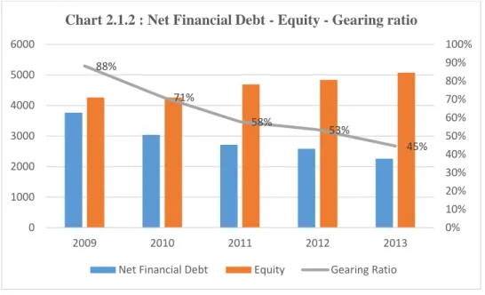
The group is constantly decreasing the amount of net financial debt. Along with the increasing market capitalization it allows to keep decreasing the gearing ratio of the company. The target value for gearing ratio is set around 50 measured in book value.

With its top-quality products, the Group is one of the leading partners to the automotive and consumer goods industries in Europe and to the oil and gas industries worldwide. The Voestalpine Group is also the world market leader in turnout technology, special rails, tool steel, and special sections. The most recent reported revenue of the group equaled to 11.5 billion EUR with the EBITDA of 1.45 billion EUR. It has around 46,400 employees worldwide.

Table 2.1.1: Key Figures

In millions of Euros _{2012 2013} Change in %(comparing to 2012)

Revenue 12,058.2 11,524.4 -4.4 EBITDA 1,301.9 1,441.8 10.7 EBITDA margin 10.8% 12.5% EBIT 704.2 853.6 21.2 EBIT margin 5.8% 7.4% Employees 46,473 46,351 -0.3

The announced dividends for 2013 equaled to 0.90 EUR per share, which is 0.10 eurocent more comparing to two previous financial years. With the net income of 444.87 million EUR, the dividend payout ratio corresponds to 34.13%, with ROE of 9.10% and sustainable growth rate of 6%. The financial year for the Groups end on the 31 of April.

88% 71% 58% 53% 45% 0% 10% 20% 30% 40% 50% 60% 70% 80% 90% 100% 0 1000 2000 3000 4000 5000 6000 2009 2010 2011 2012 2013

Chart 2.1.2 : Net Financial Debt - Equity - Gearing ratio

The portfolio of products supplied by the group is highly diversified; it includes more than 600 different units. The key industries generating most of the revenue for the group are automotive, energy industry, railway infrastructure and civil & mechanical engineering.

Even though geographically the group is represented all over the world, the largest portion of the revenue comes from the customers located in European Union. Overall 72% of sales are attributed to this region. The rest portion is allocated almost equally among Brazil, United States, Asia, Eastern Europe and Rest of the World. However, within the European Union customers there are many oriented on export to emerging markets. Therefore, despite the fact that local region is key consumer for the Group, it also can be said that developing economies have a substantial impact on sales.

29% 16% 2% 13% 11% 5% 9% 2% 13%

Chart 2.1.2: Revenue by industry

Automotive Energy industry Storage technology Railway infrastructure

Civil and mechanical engineering White good/consumer good

Building and construction subsuppliers Aviation

Voestalpine Group comprises of four divisions, which are Steel Division, Special Steel Division, Metal Forming Division and Metal Engineering Division. Steel Division was always the main part of the Group, therefore it is not surprising that it shows leading values in revenue generation.

On 19 of December 2012 Voestalpine Group Strategy 2020 was adopted. The document states the plan of development for the Group in terms of technological expansion of existing facilities, the targeted operational performance, which must direct Voestalpine AG to the leading position in mobility and energy segments. According to the plan, the Group is expecting to increase its total revenue to 2 billion EUR by the year 2020. In order to achieve those goals, it is scheduled to investment in production expansion from 800 million EUR to 1 billion EUR each year till 2020.

72% 5%

5% 8%

6% 4%

Chart 2.1.3: Revenue by regions

European Union Other Europe Brazil North America Asia

Rest of the world

33%

23% 25%

19%

Chart 2.1.4: Revenue by division

Steel Division Special Steel Division Metal Engineering Division Metal Forming Division

Steel Division

The Steel Division produces and processes hot and cold rolled steel as well as electro galvanized hot-dip galvanized, and organically coated plate. Its other activities include electrical steel strip, heavy plate

production, a foundry, and a number of downstream sectors—the Steel Service Center, pre-processing, logistics services, and mechatronics, which are all managed as independent companies.

Voestalpine Group is top European supplier of highest quality steel strip and global market leader in heavy plate for the most sophisticated applications as well as casings for large turbines. The Voestalpine Steel Division is a strategic partner for Europe’s well known automobile manufacturers and major automotive suppliers. Among the key customers there are such giants of automobile industry as Daimler AG, Volkswagen AG, Bayern Motoren WK and FIAT SPA. Additionally, it is one of the largest suppliers to the European consumer goods and white goods industries as well as to the mechanical engineering sector. Voestalpine produces heavy plate for energy sector that is used under extreme conditions in the oil and gas industries, for example, for deep-sea pipelines or in the permafrost regions of the world. Furthermore, the division is a global leader in the casting of large turbine casings. (Voestalpine AG, 2013)

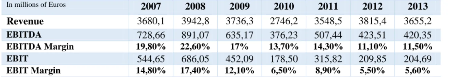
Table 2.2.1 In millions of Euros _{2007 2008 2009 2010 2011 2012 2013} Revenue 3680,1 3942,8 3736,3 2746,2 3548,5 3815,4 3655,2 EBITDA 728,66 891,07 635,17 376,23 507,44 423,51 420,35 EBITDA Margin 19,80% 22,60% 17% 13,70% 14,30% 11,10% 11,50% EBIT 544,65 686,05 452,09 178,50 315,82 209,85 204,69 EBIT Margin 14,80% 17,40% 12,10% 6,50% 8,90% 5,50% 5,60%

In the business year 2012/2013, the Steel Division faced declining prices overall, therefore, revenue fell by 4.2%. However, the operating result was managed to be kept stable, which is reflected in increased EBITDA and EBIT margins. Even though the margins increased slightly, the figures themselves performed lower results comparing to preceding year.

Steel Division is highly dependent on automotive energy and constructions industries. All together these 3 segments represent 71% of total sales of the division.

33% 22% 16% 7% 5% 17%

Chart 2.2.1: Steel Division Revenue by industry

Automotive Energy industry

Building and construction subsuppliers Civil and mechanical engineering White good/consumer good Other

Special Steel Division

The division manufactures steel long products, narrow strip, forgings and special steel forgings. The Special Steel Division is global market leader in tool steel, special alloys for the oil and gas exploration and materials for blades for gas and steam turbines. With highspeed steel and valve steel, the group is the world's No. 2. With structural parts and engine pulleys for the aviation Böhler-Uddeholm is a leading provider. The voestalpine Special Steel Division is the leading global manufacturer of high performance metals, which have specially developed material properties with regard to high resistance to wear, polishability, and toughness. Customers for these materials are the automotive and consumer goods industries in the segment of tool steel applications as well as the power plant construction industry and the oil and gas industries in the segment of special components. The division is also a leading supplier of forgings for the aviation and power generation industries. (Voestalpine AG, 2013)

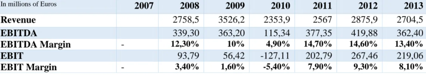
Table 2.3.1 In millions of Euros _{2007 2008 2009 2010 2011 2012 2013} Revenue 2758,5 3526,2 2353,9 2567 2875,9 2704,5 EBITDA 339,30 363,20 115,34 377,35 419,88 362,40 EBITDA Margin - 12,30% 10% 4,90% 14,70% 14,60% 13,40% EBIT 93,79 56,42 -127,11 202,79 267,46 219,06 EBIT Margin - 3,40% 1,60% -5,40% 7,90% 9,30% 8,10%

The decrease in revenue by almost 6% is attributed to the decline of production and delivery volumes. As a result of decrease in revenue and fall of EBIT margin, the operating income of the company lost almost 50 million EUR comparing to previous year.

Special steel products are more oriented on civil and mechanical engineering, than products of Steel Division. As the result 21% of revenue comes from civil and mechanical engineering for this division. Also, it is important to remark that 5% comes from supply of product for aviation industry.

25% 15% 5% 21% 12% 5% 13%

Chart 2.3.1: Special Steel Division

Revenue by

Automotive Energy industry

Building and construction subsuppliers Civil and mechanical engineering White good/consumer good Aviation

Metal Engineering Division

This division has the world’s widest range of high-quality rails and switch products, rod wire, drawn wire, prestressing steel, seamless tubes, welding filler materials and semi-finished products. The division also offers complete service packages for railway construction, including planning and engineering, transport, logistics and system installation. The Metal Engineering Division of voestalpine also has access to its own high-quality steelmaking facilities.

The voestalpine Metal Engineering Division has developed a leading position on the global railway market with its ultra-long, head-hardened HSH rails with a length of up to 120 meters. Furthermore, the division is the largest global provider of highly developed turnout systems as well as track-based monitoring systems for all railway applications. The division also has a leading market position in Europe in the specially treated wire segment, for sophisticated seamless tubes for the oil and gas industries worldwide, and high quality welding consumables. (Voestalpine AG, 2013)

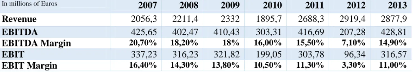
Table 2.4.1 In millions of Euros _{2007 2008 2009 2010 2011 2012 2013} Revenue 2056,3 2211,4 2332 1895,7 2688,3 2919,4 2877,9 EBITDA 425,65 402,47 410,43 303,31 416,69 207,28 428,81 EBITDA Margin 20,70% 18,20% 18% 16,00% 15,50% 7,10% 14,90% EBIT 337,23 316,23 321,82 199,05 303,78 96,34 316,57 EBIT Margin 16,40% 14,30% 13,80% 10,50% 11,30% 3,30% 11,00%

Meanwhile the insignificant decrease was faced in revenues by division, the key figures representing operating results performed outstanding increase. EBITDA and EBIT doubled and tripled correspondingly. For instance, operating income increased by approximately 210 million EUR.

Metal Engineering Division is focused on high quality rails production, which explains that 52% of output goes to railway infrastructure. Analogous to other divisions, Metal Engineering Division is also highly relies on energy and automotive industries, which in sum represent 30% of revenues for division.

12% 18% 1% 52% 7% 1% 3% 6%

Chart 2.4.1: Metal Engineering Division Revenue by customers

Automotive Energy industry Storage technology Railway infrastructure

Civil and mechanical engineering White good/consumer good

Building and construction subsuppliers Other

Metal Forming Division

The division is leading global provider of high-quality metal processing solutions in the segments of special sections, precision steel strip, and special components for the automotive and aviation industries.

The voestalpine Metal Forming Division is a leading global provider of customer specific special and precision sections as well as solutions for section systems in the construction, cab construction for commercial vehicles, and aviation sectors. The division supplies the automobile industry with both sophisticated body skin pressed parts and highly innovative structural parts and safety components. The division also produces cold-rolled, special, precision thin strips and provides one-stop solutions in the segment of high-bay warehousing systems,system racks and road safety and also operates in the energy and heating industry. Table 2.5.1 In millions of Euros _{2007 2008 2009 2010 2011 2012 2013} Revenue 1789,9 2086,2 2126,3 1552,5 2147,1 2441,9 2279 EBITDA 263,80 301,50 261,49 142,63 276,44 273,49 252,97 EBITDA Margin 14,74% 14,45% 12% 9,19% 12,88% 11,20% 11,10% EBIT 188,10 218,90 167,51 51,49 179,30 183,14 166,37 EBIT Margin 10,51% 10,49% 7,88% 3,32% 8,35% 7,50% 7,30%

Despite non-recurring effects in the amount of 10 million EUR which increased financial figures of division, revenue has declined significantly by 6.67%. The drop in performance is generally due to weaker economy and specific development of the division’s most important customer industries. Profit from operations fell from 185.1 million EUR to 167.6 million EUR.

Group, belongs to Metal Forming Division. For this part of the group, automotive customers represent 50% of sales. 50% 6% 5% 8% 3% 13% 15%

Chart 2.7:Metal Forming Division Revenue by industry

Automotive Energy industry Storage technology

Civil and mechanical engineering White good/consumer good

Building and construction subsuppliers Other

Industry Overview

To accurately estimate growth rate for Voestalpine AG prospect revenue it is necessary to analyze industry trends deriving Group’s operations. From previous paragraphs it is seen that there are more than 8 sub-sectors determining sales for Voestalpine AG. However, the major part of the returns belongs to mobility and energy industries. Mobility industry includes aviation industry, automotive and railway infrastructure, totaling 44% of revenue. Meanwhile energy industry has 16% share of Groups operations. Moreover, according to the Voestalpine Group Strategy 2020, the estimates of revenue attributed to these 2 industries will increase.

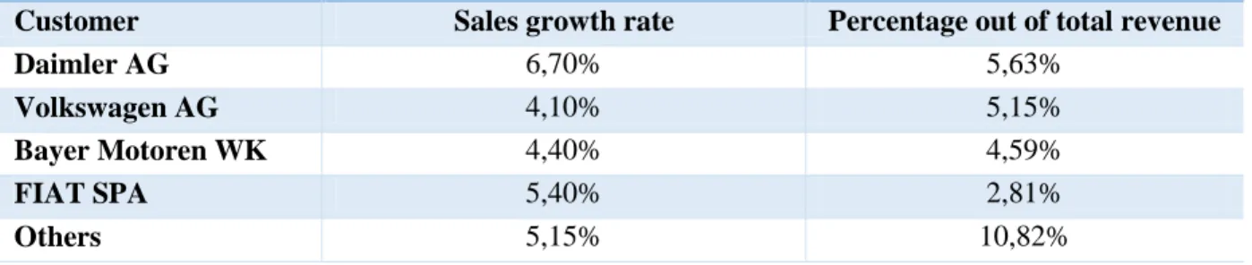
Automotive industry includes the companies which are involved in manufacture of motor vehicles. Voestalpine AG supplies doors, bonnets, boot lids, tail-hates and other body parts for different automotive manufacturers. The main customers of the Group are Daimler AG, Volkswagen AG, Bayern Motoren WK and Fiat SPA. As the supply of components for the clients is determined by their sales projections, it was assumed that the revenue growth rate for automotive segment will be driven by the forecasted sales growth rates of customers. The table below represents the share of revenue attributed to each client and their anticipated sales growth rate presented by Bloomberg. For the sales growth for smaller companies, represented in the column “Others” the average sales growth rate was considered.

Table 3.1 Automotive Industry Estimates

Customer Sales growth rate Percentage out of total revenue

Daimler AG 6,70% 5,63%

Volkswagen AG 4,10% 5,15%

Bayer Motoren WK 4,40% 4,59%

FIAT SPA 5,40% 2,81%

Others 5,15% 10,82%

As automotive segment represents 29% of total revenue for Voestalpine AG, the weighted average customers’ sales growth was calculated, which were assumed as the segment’s growth rate. As the result the value of 5.17% was estimated, which corresponds to specialists’ expectations regarding automotive industry with the growth rate of 5%-5.5%.

Table 3.2 Automotive Industry Sales Growth Rate

Customers WA contribution

to segment

Weighted growth rate for customer

WA growth for automotive industry Daimler AG 19,41% 1,30% 5,17% Volkswagen AG 17,76% 0,73% Bayer Motoren WK 15,83% 0,70% FIAT SPA 9,69% 0,52% Others 37,31% 1,92%

The sales attributed to aviation industry are linked to the sales of special components to Boeing. Therefore, analogically to automotive industry, the growth rate for aviation segment is connected to Boeing sales growth rates. Thus, the average historical growth rate of 7.54% was estimated. The calculations are presented in the Appendix.

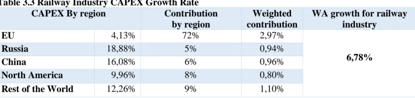
The revenue growth rate related to railway infrastructure is estimated based on the anticipated CAPEX of main players in the industry. These estimations included major railway companies of EU, Russia, China and North America. The detailed calculations related to CAPEX growth rates are attached to Appendix of the report. The final results are represented in the table below.

Table 3.3 Railway Industry CAPEX Growth Rate

CAPEX By region Contribution

by region

Weighted contribution

WA growth for railway industry EU 4,13% 72% 2,97% 6,78% Russia 18,88% 5% 0,94% China 16,08% 6% 0,96% North America 9,96% 8% 0,80%

Rest of the World 12,26% 9% 1,10%

As it is seen the emerging markets are investing significantly more comparing to EU. The main reason is that developing economies are constructing new and expanding old railways, while EU CAPEX is mostly associated with replacement of depreciated assets. Moreover, the European railways observe declining trend in investments. Even though local market for Voestalpine AG reflects 72%, extremely high growth rates in foreign markets allow the Group to assume the growth rate of 6.78%.

For the energy industry the Group is supplying special components for construction of oil and gas exploring facilities, such as heavy plates and deep-see pipelines for permafrost regions. Therefore, the sales of Voestalpine AG attributed to energy industry are determined by the investments in PPE by oil and gas companies. So, with the purpose of calculating CAPEX rate, the largest oil and gas companies of different regions were analyzed. All in all, the sample included 10 EU companies, 4 Russian, and 3 for China, Brazil and North America. The highest investment growth rates are observed in Brazil and Russia with 28.23% and 18.86% respectively. However, these regions represent only 10% of Voestalpine AG sales. The EU with 72% of Group’s revenue and on average with 12.91% CAPEX increase for regions’ companies, is determinant in weighted average growth rate of 14% for revenue related to the segment. The full data on calculations and companies is presented in the Appendix.

Table 3.4 Energy Industry CAPEX Growth Rate

CAPEX By region Contribution

by region WA WA growth for energy industry EU 12,91% 72% 9% 14% Russia 18,86% 5% 1% China 13,73% 6% 1% Brazil 28,23% 5% 1% North America 11,26% 8% 1%

Rest of the world 17,00% 4% 1%

The rest of the industries operated by the Group are assumed to move with in relation to anticipated world’s nominal GDP. For instance, the building and construction industry is considered to be highly related to the economic growth rate. The same can be stated about the storage industry. Thus, the projected world’s nominal GDP by IMF is 5.7%. (http://www.imf.org/external/ns/cs.aspx?id=28). The table below represents the growth rates for the industries supplied by Voestalpine AG.

Table 3.5 Industries’ Growth Rates

Industry Estimated growth rate

Automotive 5,17%

Energy industry 14,05%

Storage technology 5,70%

Railway infrastructure 6,78%

Civil and mechanical engineering 5,70%

White good/consumer good 5,70%

Building and construction subsuppliers 5,70%

Aviation 7,54%

Cost of Capital

The weighted average cost of capital for Voestalpine AG is calculated based on the data available on 11.12.2013, the starting date of the valuation. With the price of 34 EUR per share and having 172.4 million shares outstanding, the market capitalization of the Group equaled to 5,861.6 million EUR. Meanwhile, the outstanding market value of debt totaled 3,419.5 million EUR. Assuming these values for the valuation the following capital structure of the group is estimated.

Cost of Debt

In October 2007, Voestalpine AG issued subordinated hybrid bond with an issue volume of 1 billion EUR and a coupon rate of 7.125%. At the end of the business year 2012/2013 the bond was traded 5% above the face value. In order to optimize its financing portfolio, in February 2013, the Group offered all existing holders of the hybrid bond 2007 the opportunity to exchange their holdings for a new hybrid bond 2013 with a volume of up to 500 million EUR. The demand for the bonds was extremely high, resulting in 9.5% premium over the face value.

In early February 2011, Voestalpine AG successfully placed a seven-year bond issue (called Corporate Bond 2011 – 2018) on the capital market with a coupon rate of 4.75% and a volume of 500 million EUR. At the end of September 2012, corporate bond 2012-2018 was issued, with the amount of 500 million EUR and the interest rate of 4%. Both of the issues are traded substantially above the face value.

Table 4.2.1 Voestalpine AG Bonds Outstanding

Bonds Coupon rate Date of issue Maturity Amount (in EUR) YTM

Corporate bond 1 4,75 03.02.2011 05.02.2018 500 000 000,00 2,789 Corporate bond 2 4 05.10.2012 05.10.2018 500 000 000,00 2,883 Hybrid bond 2007 7,125 31.10.2007 29.10.2049 500 000 000,00 5,255 Hybrid bond 2013 7,125 / 6 20.03.2013 29.12.2049 500 000 000,00 5,422

63,16%

36,84%

Chart 4.1.1: Voestalpine AG

capital structure