UNIVERSIDADE DE LISBOA FACULDADE DE CI ˆENCIAS DEPARTAMENTO DE F´ıSICA
ON THE HOT INTERSTELLAR MEDIUM OF
HIGH-REDSHIFT GALAXIES
Lara Sofia Gorgulho Alegre
MESTRADO EM F´ıSICA
Especializa¸c˜ao em Astrof´ısica e Cosmologia
Disserta¸c˜ao orientada por:
Prof. Doutor David Ricardo Serrano Gon¸calves Sobral
Abstract
At high redshift, galaxies are very different from the ones in the local Universe. They present several high ionization ultraviolet emission lines such as Civ, Oiii] and Ciii], besides Heii which is associated with young and massive stars. The energy required for the production of emission lines like Civ was once only associated to Active Galactic Nuclei (AGNs). However, photoionization models have shown that these lines can be produced by star forming galaxies (SFGs) holding very hot and young stellar populations with a low metal content.
The properties of high-redshift galaxies are not fully understood and the discrimination be-tween these galaxies and AGNs is essential for their understanding. Recently, diagnostic diagrams using ultraviolet emission lines started being developed, however they are based on single stellar populations, which cannot reproduce the spectral energy distribution of these galaxies.
In this work we produce and present three sets of models of nebular emission that allow to interpret and distinguish SFGs and AGNs, using the photoionization simulation code cloudy.
We created a set of cloudy models using black bodies with a broad range of temperatures (20000 - 150000 K), densities (102 - 105 cm−3) and metallicities (1− 10−5 Z
), which span from
ionization parameters logU ∼ -1 to -4.5. This provides a set of models with well known input parameters. Models below ∼ 70000K can reproduce SFGs while the ones with higher temperature go into the classical AGN regime.
To simulate AGNs we create another set of models based on power laws with slopes from -1.2 to -2.0 within the same range of densities and metallicities.
Thirdly, for SFGs we used the state-of-the-art binary stellar evolutionary models bpass.v2 (Bi-nary Population And Spectral Synthesis code). It is thought that at least ∼ 70% of stars live in binary systems. Binary interactions which account for rotation effects are extremely important to understand the spectral energy distribution of these galaxies. In particular, for low metallicity sys-tems, at which binary interactions promote dynamically mass transfer between the stars contrarily to high metallicity systems where the binary tends to become a wide structure.
We present emission-line ratios diagnosis diagrams based on Ciii], Oiii], Civ and Heii] using our photoionization models. These diagrams allow to discriminate between SFGs and AGNs and at the same time provide a tool for unveiling the physical properties of these sources.
We apply the modelling results to a population of 10 analogues of high redshift galaxies at z∼ 2 - 3 selected by their UV continuum. We found that these galaxies are better described by our bpass models holding young stellar populations with ages∼ 106.4 - 106.8 yrs, ionization parameters ∼ logU = -2.21 , low stellar metallicities ∼ 0.2 - 0.1 Z and very low gas metallicities ∼ 0.004 Z .
[Oii], Hα and Hβ. These emission line fluxes can probe metal poor SFGs at high redshift to be observed with upcoming telescopes such as the James Webb Space telescope, and further test the validity of bpass models to explain these sources.
We then analyse 6 bright Lyα emitters at the same range of redshifts, and we found that 3 of these systems are also better described by our bpass models. They are consistent with being analogues of high redshift galaxies, in particular 2 galaxies which present young ages (∼ 106.3- 106.5 yrs), higher ionization parameter (logU = -1.84 to -1.74) and lower stellar metallicity (< 0.1 Z )
than the previous UV continuum selected galaxies.
We then use our models to understand the absence of metal lines in bright LAEs at redshifts up to z = 6 - 7, and we conclude that most of these sources require deeper observations.
Lastly, we analyse galaxies from the HiZELS survey, selected with narrow band filters by their bright Hα emission line. We analyse a total of 425 spectra obtained with follow-up VIMOS (VLT) spectroscopy and we calculated the spectroscopic redshifts of 87 galaxies and AGNs. We found bright ionization ultraviolet lines in 2 of these galaxies at z ∼ 1.5 and we estimate that these galaxies present extreme properties similar to the z∼ 2 - 3 bright LAEs analysed before.
Our models provide a tool to discriminate between the nature of the galaxies, and estimate their physical properties. Our results are highly important to understand the properties of young galaxies now being found at the epoch of reionization.
We aim to make all our modelling results fully public so it can benefit a wider community. Keywords: galaxies: evolution; high-redshift; Interstellar medium; emission lines; observations.
Part of this work has been submitted or is in preparation for submission to the Monthly Notices of the Royal Astronomical Society:
• “Spectroscopic properties of luminous Lyman-α emitters at z ≈ 6 − 7 and comparison to the Lyman-break population.” Matthee, Jorryt, David Sobral, Behnam Darvish, S´ergio Santos, Bahram Mobasher, Ana Paulino-Afonso, Huub R¨ottgering, and Lara Alegre. arXiv preprint arXiv:1706.06591 (2017).
• Sobral et al. in prep (including Lara Alegre), “The nature and diversity of luminous Lyα emitters at z = 2 - 3: an extremely ionising population”
Resumo
Gal´axias distantes, a elevado “redshift”, apresentam caracter´ısticas muito diferentes das gal´axias do Universo local. S˜ao gal´axias pequenas e compactas, por vezes com formas bastante irregulares e muitas vezes em processos de fus˜ao com outras gal´axias. Estas gal´axias contˆem maioritariamente popula¸c˜oes estelares jovens, dominadas por estrelas massivas que produzem elevada quantidade de fot˜oes ionizantes. Espera-se que alberguem tamb´em as primeiras gera¸c˜oes de estrelas (popula¸c˜ao III). O seu elevado n´umero a alto redshift bem como a energia que produzem leva-as a serem consideradas as respons´aveis pela reioniza¸c˜ao do Universo.
No espetro destas gal´axias ´e poss´ıvel observar riscas de emiss˜ao ultravioleta, caracter´ısticas de estrelas massivas, como Heiiλ1640 ˚A, Ciii]λλ1907,1909 ˚A, Civλλ1948,1951 ˚A e Oiii]λλ1661,1666 ˚
A. Estas riscas requerem elevadas energias de ioniza¸c˜ao, sendo mais comuns em gal´axias a elevado redshift. No entanto, a redshift aproximadamente entre 2 e 3, v´arias observa¸c˜oes indicam existir uma popula¸c˜ao de gal´axias com caracter´ısticas semelhantes. S˜ao gal´axias compactas, com altas taxas de forma¸c˜ao estelar, baixa metalicidade e riscas de emiss˜ao semelhantes. Nesta gama de redshifts as linhas de alta ioniza¸c˜ao ultravioleta destas gal´axias est˜ao deslocadas para comprimentos de onda no ´otico, o que permite observ´a-las com telesc´opios localizados no solo.
Estudar estas gal´axias ajuda-nos a compreender gal´axias a elevado redshift e permite-nos desen-volver meios de diagn´ostico para identificar as suas caracter´ısticas e compreender a sua natureza. Estes meios de diagn´osticos ser˜ao ´uteis para estudar gal´axias a elevado redshift cujas linhas ul-travioleta est˜ao deslocadas para comprimentos de onda maiores, sendo melhor observadas a partir do espa¸co. Novos telesc´opios, como por exemplo o James Webb Space Telescope, ter˜ao a capaci-dade de observar espetros de milhares de gal´axias at´e redshifts perto de 10. No entanto existe j´a a necessidade de compreender gal´axias encontradas no final da ´epoca da reioniza¸c˜ao (redshifts aproximadamente entre 6 e 7) como ´e o caso da gal´axia CR7, que apresenta apenas Lyα e Heii indi-cando uma popula¸c˜ao de estrelas com elevada grande capacidade de ioniza¸c˜ao e baixa metalicidade, por exemplo uma popula¸c˜ao III de estrelas. No entanto os meios de diagn´ostico que existem n˜ao conseguem explicar as riscas de emiss˜ao observadas nestas gal´axias.
Muitas vezes estas gal´axias produzem energias de ioniza¸c˜ao associadas a AGNs (“Active Galac-tive Nuclei”, buracos negros ativos que ejetam material at´e Mega parsecs de distˆancia). Distinguir gal´axias com tais caracter´ısticas de AGNs n˜ao ´e f´acil. Para gal´axias a baixo redshift e com pro-priedades semelhantes `as gal´axias do Universo local, este tipo de diagn´ostico j´a existe, usando por exemplo, raz˜oes entre linhas de emiss˜ao do espetro vis´ıvel, como ´e o caso do diagrama BPT. Diagra-mas de diagn´ostico recorrendo a linhas ultravioleta tendo em conta os fluxos de emiss˜ao detetados nestas gal´axias s´o agora come¸caram a ser desenvolvidos.
Neste projeto utilizamos ao c´odigo de fotoioniza¸c˜ao cloudy para simular as condi¸c˜oes f´ısicas caracter´ısticas deste tipo de gal´axias, bem como em AGNs. O cloudy determina as condi¸c˜oes f´ısicas de um g´as irradiado por uma fonte de ioniza¸c˜ao externa, resolvendo numericamente as equa¸c˜oes de equil´ıbrio estat´ıtisco, conserva¸c˜ao de carga e de energia. O cloudy permite definir diversas condi¸c˜oes, quer para a fonte de ioniza¸c˜ao, quer para as propriedades do g´as que rodeia estas fontes. Como output, o cloudy determina por exemplo o n´ıvel de ioniza¸c˜ao, as condi¸c˜oes qu´ımicas do g´as, a temperatura e gera centenas a milhares de linhas de emiss˜ao.
Para criar os nossos models usamos diferentes geometrias (esf´erica para simular gal´axias e plano paralela para simular AGNs) e v´arias condi¸c˜oes de densidade e baixa metalicidade, tendo em conta que as abundˆancias dos elementos carbono e azoto n˜ao variam linearmente com a metalicidade do g´as.
Foram criados trˆes tipos de modelos com fontes de ioniza¸c˜ao diferentes: um corpo negro com temperaturas entre 20000K a 150000K, que permite simular o comportamento tanto de uma gal´axia com forma¸c˜ao estelar como de um AGN (a temperaturas e condi¸c˜oes de ioniza¸c˜ao mais elevadas); uma lei de potˆencia com diferentes expoentes, que permite modelar AGNs; e distribui¸c˜oes espectrais de energia baseadas em forma¸c˜ao estelar (modelos bpass), que permitem simular de uma forma mais realista gal´axias com forma¸c˜ao estelar.
Enquanto a energia produzida por uma lei de potˆencia ou por um corpo negro permite simular condi¸c˜oes sem incertezas inerentes a modelos de AGNs ou modelos estelares, para interpretar o seu espetro de emiss˜ao de uma gal´axia de forma precisa ´e necess´ario recorrer a modelos de evolu¸c˜ao sint´etica (ES), tamb´em referidos muitas vezes como popula¸c˜oes sint´eticas estelares (SPS).
Existe um grande n´umero de modelos de evolu¸c˜ao sint´etica, que podem variar, de uma forma geral, de modelos te´oricos que incluem processos de evolu¸c˜ao estelar a modelos emp´ıricos. Con-tudo, modelos de evolu¸c˜ao sint´etica convencionais n˜ao conseguem explicar os fluxos caracter´ısticos destas gal´axias. Por essa raz˜ao, evolu¸c˜ao estelar e evolu¸c˜ao gal´atica criaram de certa forma uma sinergia. Novos modelos de evolu¸c˜ao sint´etica que incluem intera¸c˜oes estelares bin´arias bem como rota¸c˜ao estelar, revelaram um grande impacto na distribui¸c˜ao espectral de energia das gal´axias, principalmente a baixa metalicidade. Estes efeitos prolongam a vida das estrelas massivas, essen-ciais para a produ¸c˜ao de fot˜oes ionizantes. Estes novos modelos de evolu¸c˜ao sint´etica s˜ao tamb´em essenciais para compreender a reioniza¸c˜ao do universo, uma vez que eles conseguem prever os fot˜oes necess´arios para a reioniza¸c˜ao. Da mesma forma, estudar gal´axias com tais caracter´ısticas tem permitido grandes avan¸cos na compreens˜ao dos processos relativos a estrelas massivas.
No nosso projeto us´amos a ´ultima vers˜ao dos modelos de evolu¸c˜ao sint´etica bpass v2.0 (Binary Population And Spectral Synthesis code) que inclui modelos estelares que tˆem em conta os efeitos descritos. Desta forma, ´e poss´ıvel descrever e interpretar de forma mais precisa as condi¸c˜oes reais destas gal´axias. Com esse objetivo, usamos os nossos modelos para reproduzir diferentes diagramas de diagn´ostico baseados em raz˜oes entre v´arias linhas de alta ioniza¸c˜ao, como Civ/Heii, Ciii]/Heii, Ciii]/Civ e Oiii]/Heii. Os nossos modelos permitem fazer um diagn´ostico das fontes, tanto a n´ıvel da sua natureza (AGNs vs SGFs) como estimar as suas propriedades. Os nosso modelos de fotoioniza¸c˜ao que utilizam os modelos de evolu¸c˜ao sint´etica bpass conseguem reproduzir condi¸c˜oes em gal´axias com baixa metalicidade que outros modelos de evolu¸c˜ao sint´etica que n˜ao incluem sistemas bin´arios n˜ao conseguem explicar.
Utilizando os nossos modelos, estudamos v´arias gal´axias, ao longo de diferentes redshifts. Os nossos modelos permitem descrever de forma mais realista as condi¸c˜oes de v´arias gal´axias encon-tradas a redshifts 2 - 3, semelhantes a gal´axias a elevado redshift.
Com base nas nossas interpreta¸c˜oes fiz´emos uma previs˜ao dos fluxos de linhas ´oticas carater´ısticos deste tipo de fontes, a serem detetadas com o James Webb Space Telescope em gal´axias a elevado redshift.
Com ferramentas que permitem analisar de forma mais precisa gal´axias com baixa metalicidade, selecion´amos e estud´amos duas gal´axias a redshift∼ 1.5 do HiZELS survey, selecionadas atrav´es da sua linha de emiss˜ao Hα, que indica alta taxa de forma¸c˜ao estelar. Estas gal´axias foram observadas com o instrumento VIMOS (Very Large Telescope) e apresentam condi¸c˜oes semelhantes a gal´axias encontradas a redshifts 2 - 3 e an´alogas a gal´axias a elevado redshift.
Os resultados obtidos s˜ao importantes para compreender e interpretar as propriedades das gal´ ax-ias a elevado redshift e ajudam a explicar a energia necess´aria para a reioniza¸c˜ao do Universo atrav´es destes pequenos e compactos sistemas.
Palavras-chave: gal´axias: evolu¸c˜ao; elevado redshift; meio interestelar; linhas de emiss˜ao; observa¸c˜oes.
Contents
Abstract I Resumo IV List of Figures IX List of Tables XI 1 Introduction 1 1.1 Lookback time . . . 1 1.2 Epoch of reionization . . . 2 1.3 First Galaxies . . . 41.3.1 Star Forming Galaxies . . . 4
1.3.2 Active Galactic Nuclei . . . 5
1.3.3 The Interstellar Medium . . . 5
1.3.4 The Spectra . . . 7
1.4 Emission line diagnosis . . . 9
1.4.1 Line-ratios as a diagnosis tool . . . 10
1.5 Searching for the first galaxies . . . 13
1.6 Modelling emission from high-redshift galaxies . . . 14
1.6.1 Photoionization Codes . . . 14
1.6.2 Evolutionary Synthesis models . . . 14
1.7 Motivation and Goals . . . 16
2 cloudy photoionization modelling 19 2.1 The gas cloud . . . 19
2.1.1 Geometry of the gas cloud . . . 19
2.1.2 Density of the gas . . . 21
2.1.3 Chemical Abundances . . . 22
2.1.4 Grains . . . 25
2.2 Other parameters . . . 26
2.2.1 CMB and Cosmic ray background . . . 26
2.2.3 Emission lines . . . 27
2.2.4 Python tools . . . 28
2.3 The radiation field . . . 29
2.3.1 Star Forming Galaxies . . . 30
2.3.2 Active Galactic Nuclei . . . 33
3 Modelling results 35 3.1 Comparison of the photoionization models . . . 35
3.2 Modelling diagnosis . . . 38
3.2.1 BPT diagram . . . 38
3.2.2 UV emission-line diagnostic ratios . . . 40
4 Application across redshift 45 4.1 Analogues of primeval galaxies at 2.4 ≤ z ≤ 3.5 . . . . 45
4.1.1 Predictions for the James Webb Space Telescope . . . 51
4.2 Bright LAEs at z ∼ 2 - 3 . . . . 52
4.3 Application to z ∼ 6 - 7 galaxies . . . . 56
5 VIMOS - HiZELS SFGs 59 5.1 HiZELS Survey . . . 59
5.2 Spectroscopic data overview . . . 59
5.3 Analysis of 2 HiZELS SFGs at z ∼1.46 . . . . 61
6 Conclusions 65
List of Figures
1.1 AGN vs SFG SEDs . . . 7
1.2 Quasar emission-line spectrum . . . 8
1.3 Energy-Level diagram for [Oiii] . . . 9
1.4 AGN and low-metallicity SFG SED comparison . . . 10
1.5 BPT diagram . . . 11
1.6 UV emission-line ratio diagram . . . 12
1.7 bpass evolutionary pathways . . . 16
2.1 cloudy geometries . . . 19
2.2 Carbon-Oxygen abundance ratio . . . 23
2.3 Nitrogen-Oxygen abundance ratio . . . 25
2.4 3MdB example . . . 29
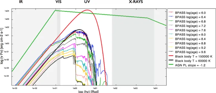
2.5 bpass Ionizing fluxes . . . 33
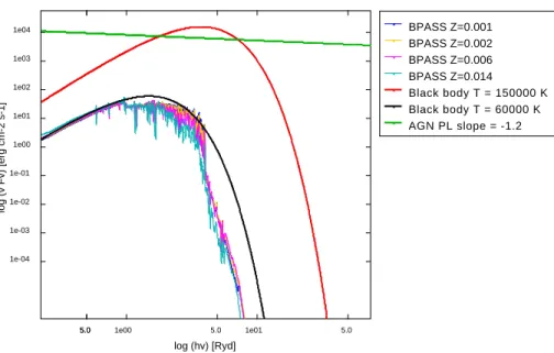
3.1 Continuum of the models in the UV range of energies . . . 36
3.2 bpass continuum for different metallicities . . . 36
3.3 Continuum for different bpass ages . . . 37
3.4 BPT diagram for all models . . . 38
3.5 BPT diagram for models with solar metallicity . . . 39
3.6 Influence of adjustable parameters on emission-line ratios . . . 40
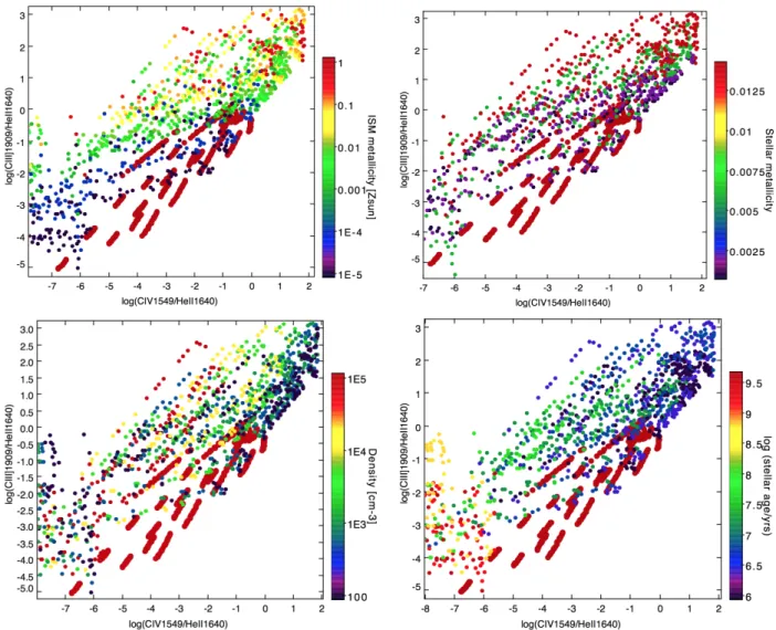
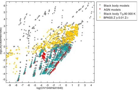
3.7 Log(Ciii]/Heii) vs log(Civ/Heii) diagram for all models . . . 41
3.8 Log(Ciii]/Heii) vs log(Civ/Heii) diagram region where AGN and bpass models overlap 42 3.9 AGN and bpass discriminator parameters . . . 43
4.1 Amor´ın et al. (2017) SFGs composite spectrum . . . 45
4.2 UV emission-line diagrams of Amor´ın et al. (2017) SFGs . . . 46
4.3 Comparison between physical parameters obtained with bpass and black body vs Amor´ın et al. (2017) results . . . 50
4.4 Carbon to helium emission line ratios for six LAEs presented in Sobral et al. (in prep) 52 4.5 Carbon and oxygen emission line diagrams of the six LAEs from Sobral et al. (in prep) 53 4.6 LAEs Civ/Lyα and C iii]/Lyα ratios . . . 57
4.7 Civ/Lyα and Ciii]/Lyα . . . 57
5.2 HiZELS - VIMOS: redshift distribution . . . 60
5.3 HiZELS - VIMOS: photometric vs spectroscopic redshifts . . . 60
5.4 HiZELS - VIMOS: SFGs spectra . . . 61
5.5 HiZELS - VIMOS: SFGs UV emission line diagnostic ratios . . . 62
C.1 Log(Ciii]/Heii) vs log(Civ/Ciii]) for all models . . . 93
C.2 Log(Civ/Heii) vs log(Civ/Ciii]) for all models . . . 94
C.3 Log(Ciii]/Heii) vs log(Oiii]/Heii) for all models . . . 94
C.4 Log(Civ/Ciii]) vs log(Oiii]/Heii) for all models . . . 95
C.5 Log(Civ/Heii) vs log(Oiii]/Heii) for all models . . . 95
C.6 AGN and SGF discriminators for all the UV line ratios . . . 96
E.1 VIMOS field-of-view . . . 99
E.2 HiZELS - VIMOS: Coordinates of the six observed pointings . . . 100
List of Tables
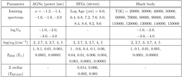
2.1 High to moderate ionization UV and Optical emission-lines . . . 28
2.2 bpass stellar metallicities . . . 31
2.3 bpass stellar ages . . . 32
2.4 AGN spectral indexes . . . 34
3.1 Photoionization parameters for AGNs and SFGs . . . 35
4.1 Properties of SFGs from Amor´ın et al. (2017) calculated with the black body models 47 4.2 Properties of SFGs from Amor´ın et al. (2017) calculated with the bpass models . . 48
4.3 Optical emission lines predictions for the James Webb Space Telescope . . . 51
4.4 Properties of LAEs from Sobral et al. (in prep) estimated with the black body models 54 4.5 Properties of LAEs from Sobral et al. (in prep) estimated with the bpass models . . 54
5.1 HiZELS galaxies: spectroscopic redshifts . . . 62
5.2 HiZELS galaxies: calculated properties using the black body models . . . 62
5.3 HiZELS galaxies: calculated properties using the bpass models . . . 63
A.1 cloudy solar composition . . . 89
A.2 PyCloudy and cloudy emission-line commands . . . 90
Chapter 1
Introduction
1.1
Lookback time
The study of galaxy formation and evolution is only possible because we live in a Universe that is in harmony with the Cosmological principle. This principle states that the Universe is homogeneous and isotropic at large scales. This has been corroborated by several observations (e.g. CMB, Cosmic Microwave Background, Penzias and Wilson (1965)), and it is also in agreement with the concordance model (ΛCDM, Cold Dark Matter Model, Ostriker and Steinhardt (1995)).
According to the ΛCDM, the Universe has a positive Λ constant, meaning that all the galaxies are receding from us (Hubble (1929)) at an accelerated rate (Riess et al. (1998)). No matter where we look up on the sky, as the light speed is finite, we are literally looking back in time. Galaxies that are at the same distance in space from us, will be at the same distance in time. This also means that there must have been a starting point in space and time (Big Bang). We can then study galaxies at different epochs of the Universe inferring its evolution across cosmic time.
In an expanding Universe the recession speed v is given by the Hubble’s law v = H0 d, where d is
the distance to the observer and H0 is the Hubble constant ( H0 = 67.8±0.9 km s−1Mpc−1, Planck
Collaboration et al. (2016)). Astronomical distances of extragalactic objects are usually described in terms of redshift (z), which is a function of the recession speed of the objects:
1 + z = s
1 + v/c
1− v/c (1.1)
The redshift results from the expansion of space itself and is related with the cosmic scale factor a(t) by:
1 + z = a(te) a(to)
(1.2) The cosmic scale factor is the relative expansion of the Universe as function of time, where a(to)
represents the size of the Universe when the light from the object is observed, and a(te) the size of
the Universe when the light was emitted. The light wave originally emitted is lengthened by the space expansion and is shifted to longer (redder) wavelengths. Therefore it can be used to calculate the redshift:
z =λo− λe λe
, (1.3)
where λ0 is the observed wavelength and λe is the emitted one.
The redshift can be used to calculate the age of an object. The evolution of the Hubble constant, which can be calculated through the Friedmann equations applied to the general relativity, evolves over time with the relation:
H(a)≡ H0
p
Ωr a−4+ Ωm a−3+ Ωk a−2+ ΩΛ , where a = a(t) =
1
1 + z (1.4)
By definition H ≡ ˙a(t)/a(t), therefore da = a H(a) dt. Integrating we can obtain the lookback time age: t = Z a 0 da a H(a) (1.5)
The age of the Universe (a = a0 = 1, z = 0) can be calculated using the last results of the
cosmological parameters (Planck Collaboration et al. (2016)): ΩΛ = 0.692± 0.012 (dark energy
density), Ωm = 0.308± 0.012 (matter density: baryons and dark matter), Ωr ∼ 10−4 (radiation
density: photons and neutrinos) and Ωk< 0.005 (spatial curvature). These are estimations for the
present day cosmological parameters and leave us with a Universe with 13.799± 0.021 Gyr.
1.2
Epoch of reionization
Because our Universe has a finite age, the size of the observable universe is also finite. The light can only reach us from distances smaller than the age of the Universe. However, during the first ∼ 400 000 million years after the Big Bang, radiation dominated and the Universe was opaque due to the Thompson scattering of the free electrons on the dense and hot plasma.
As the Universe expanded and cooled, matter started to dominate over radiation and almost all free electrons and protons combined to form neutral hydrogen atoms. This process is known as “recombination” (even though electrons and nuclei had never been “combined” before) and occurred at z = 1100. After the recombination, the universe became transparent to the CMB (i.e. the photons that were last scattered at that time).
According to the CMB measurements, the Universe was essentially homogeneous. However, tiny fluctuations in density and temperature became bigger with time as the gravitational forces were also slightly stronger than in other regions. Overdense regions of space started to collapse under gravity and stopped to expand. Dark matter may have played here a major role since baryonic matter could not collapse efficiently by itself.
The first stars and galaxies did not start to form before z ∼ 50 − 20, during the “Dark Ages”, inside mini dark matter haloes. These very first galaxies produced high-energy photons, ionizing the diffuse hydrogen in their immediate surroundings, and beginning a progressive process that culminated with the full “reionization” of the Universe.
Planck Collaboration et al. (2016) estimated an instantaneous reionization at z ∼ 8.8+1.2−1.1. Several observational constrains place it 6 . z . 10 (e.g. Robertson et al. (2015)), while other
observations indicate that the process was essentially completed by z ∼ 6, because the number density of neutral hydrogen clouds increases above that redshift (e.g. Fan et al. (2006), Stark et al. (2015)).
Furthermore observations have also shown that it was not an homogeneous process but rather occurred in preferred regions, being a patchy process (e.g. Matthee et al. (2015), Sobral et al. (2015)). This also supports the idea that reionization started around strong ionizing sources that created bubbles of ionized hydrogen in their vicinity. Ionized regions gradually overlapped each other and the typical distances travelled by the ionizing photons grew rapidly, which led to a largely ionized intergalactic medium (IGM) with smaller regions of moderate overdense gas.
One of the main questions in astrophysics and cosmology is the understanding of the cosmic epoch of reionization and the physical processes responsible for it. The transition of the Universe from neutral to ionized is associated with the presence of photons with energies higher than 13.6 eV (λ < 912 ˚A, ultraviolet light (UV)) produced by the first stars and galaxies. However, the physics behind the escape fraction of hydrogen ionizing photons (fesc) is not completely understood (e.g.
Hayes (2015)) and the process is complex from both theoretical (e.g. Robertson et al. (2015)) and observational (e.g. Sobral et al. (2017)) perspectives.
Furthermore, the state of ionization is determined by the balance between the rate of hydrogen recombination and photoionization, where the number of ionizing photons is crucial to maintain the ionization state of the Universe. Studies of local metal poor galaxies can help understanding the problems inherent to the escape fraction (e.g. Izotov et al. (2016)).
Cosmic reionization drivers
Star-forming galaxies (SFG) and Active Galactic Nuclei (AGN) have always been pointed as the main drivers for cosmic reionization, since they are strong ionizing sources. Their relative contributions to the total UV emission across cosmic time is still uncertain; however, SFGs have been favoured as the main contributors at early times (e.g. Robertson et al. (2015), Bouwens et al. (2015)) and the ones responsible for conserving the ionization state of the Universe (e.g. Fan et al. (2006), Haardt and Madau (1996)). AGNs by themselves are not enough to reionize the Universe and maintain the hydrogen reionization higher mainly because at z & 3 the number density of bright AGNs drops (e.g. Masters et al. (2012)). While bright AGNs are known to exist at z > 7 (e.g. Mortlock et al. (2011)), their UV luminosity function declines rapidly between z ∼ 4 and z ∼ 6 (e.g. Parsa et al. (2017)). At z ∼ 6 the AGN contribution for the total UV luminosity budget is an order of magnitude smaller than the level required to maintain the ionization state against hydrogen recombination (Parsa et al. (2017)). However, the faint-end slope of the AGN luminosity function remains uncertain and their role in the reionization process is not completely understood (e.g. Kim et al. (2015)).
It has been possible to measure the galaxy UV luminosity function out to z∼ 10 (e.g. Bouwens et al. (2015)), which points towards a rapidly growing population of early star forming galaxies that could have produced the UV photons necessary for the reionization and its maintenance. Galaxies detected at high-redshift present hard ionizing spectra (e.g. Stark et al. (2015)), suggesting that they may be more common during the reionization and hence very different from the galaxies at
lower redshifts. Some exceptions are extremely metal poor galaxies recently found at redshifts 2 -3 (e.g. Amor´ın et al. (2017), Vanzella et al. (2016)). Moreover, Ma et al. (2016) studied the effect of stellar binary evolution (using bpass evolutionary synthesis; see Section 1.6.2) on the production of ionizing photons and on the escape fraction and concluded that the later time photons easily escape, increasing the escape fraction, in particular for low-metallicity galaxies. For single stellar models fesc ∼ 5%, less than the 20 % required by models of cosmic reionization (e.g. Robertson
et al. (2015)). The effective escape fraction to the IGM (i.e. the ratio between the ionizing flux and the continuum flux at 1500 ˚A) is boosted by factors of ∼ 4 − 10 using bpass models (Ma et al. (2016) indicating that fesc from SFGs are in agreement with the values required to ionize the
Universe. It is then necessary to understand the properties of the first galaxies, characterize their contribution with energetic UV photons at early times and estimate also the fraction of ionizing hydrogen photons that escaped to the IGM.
1.3
First Galaxies
The light emerging from a galaxy is a combination of stellar and gas emission, processed by intervening dust. However the presence of a supermassive black hole (SMBH) in the central regions of the galaxies can produce one of the most powerful energy sources in the Universe, which cannot be attributed to the normal components of galaxies: an AGN.
The first galaxies should have been very different from the galaxies at lower redshift. Images from the Hubble Deep Field (Beckwith et al. (2006)) show small and irregular galaxies that probably underwent through periods of multiple mergers to form larger galaxies like the Milky Way.
Considering the lack of sufficient confirmed high redshift galaxies beyond z∼ 6 and the qualita-tive change in the galaxy population relaqualita-tive to lower redshifts, it is very difficult to constrain and distinguish the properties of high redshift AGNs and SFGs.
1.3.1 Star Forming Galaxies
The first galaxies should be a combination of different populations of stars, with different ages, which are dominated by the hot and massive stars, that spend most of their lives with effective temperatures above 104 K, hence emitting in the UV.
In a young universe, where heavy elements had yet to be formed, the first generation of stars (Population III, POP III) formed by the collapse of gas clouds made of hydrogen and helium (and their isotopes) with traces of lithium (e.g. Glover (2011)).
The cooling processes are extremely dependent on the metal content of the gas, occurring mainly through the de-excitation of collisional excited metal transitions because hydrogen and helium re-quire high energies for collisional excitation from the ground state (> 10.2 eV). This implies high temperatures for cooling processes to occur and high Jean mass of gas (minimum mass to collapse under gravity, which is proportional to the square of the temperature) to contract and subsequent collapse into stars. For that reason it is expected that the first stars were very massive, with hun-dreds of solar masses (e.g. Abel et al. (2000)), with very low metallicity (≤ 10−4Z , Schneider
et al. (2002)) and short-lived that evolved rapidly into Type-II supernovae enriching the interstellar medium (ISM). The enriched ISM can cool more efficiently forming POP II stars, less massive and metal-poor stars. Ultimately it forms POP I stars, smaller, metal-rich and longer lived.
Recent studies have shown that 70 % of massive stars are expected to live in binary systems where stars interact with each other (e.g. de Mink et al. (2013)). It is therefore important to take into account binary evolution and rotation, in particular, because they are more accentuated at low metallicities (Eldridge et al. (2008), Stanway et al. (2014)). Binary effects can extend the lifetime of massive stars, producing UV photons during more time, which justifies the hard radiation fields found at high-redshift galaxies and which can help to unveil its true contribution for the reionization (Stanway et al. (2016)) .
One of the most fundamental observables of galaxy evolution is its star formation rate. To understand star formation in the first galaxies it is necessary to understand how efficiently these galaxies form stars, which depends on the cooling processes and on the density and metallicity of the gas; the stellar Initial Mass Function (IMF), which describes the fractional distribution in mass of a newly formed stars (Salpeter (1955)); and the stellar feedback.
Comparing the ionizing flux from high redshift galaxies with binary evolutionary synthesis mod-els show variations in the Initial Mass Function (Stanway (2017)). POP III IMF is expected to be top-heavy compared to that of Milky Way stars (Johnson (2013)) due to several physical processes (Bromm and Yoshida (2011)) and it is critical for the amount of metals that they release into the ISM (Heger and Woosley (2002)).
1.3.2 Active Galactic Nuclei
AGNs are compact objects with highly variable luminosities over short timescales and with an emission highly polarised. With a superheated accretion disk and relativistic jets that can extend to hundreds of kiloparsecs, these galaxies can reach extremely high brightness radiating across all the spectrum. Many efforts have been made to understand and characterize the formation and growth of the SMBHs. While most studies focus on the peak of both galaxy and SMBH growth at z = 1 – 4, how the first SMBHs formed and grew is not exactly known. They can have been formed through the first generations of POP III stars (e.g. Volonteri and Rees (2006), Alvarez et al. (2009)), which with a mass of 10 - 100 M can end their life as a black hole (which requires that POP III must
grow rapidly shortly after they have formed); or directly collapsing from the primordial gas clouds producing masses of 104− 106 M (e.g. Bromm and Loeb (2003)), where then they can grow to
higher masses through periods of merging and/or high accretion rates (Di Matteo et al. (2012)) to achieve masses of 109 M of the currently known z > 6 SMBHs ( e.g. Mortlock et al. (2011)).
1.3.3 The Interstellar Medium
The Interstellar Medium (ISM) is the material for the star formation. Its chemical evolution is intrinsically related with its stellar content. However, the ISM can also reveal the stellar effects on its environment, for example, the energy released by massive stars can be measured through the energy content of the surrounding ISM. There is a vast information that can be revealed by the ISM, such as the chemical composition, temperature, velocities, ionization mechanisms, etc.
The ISM is composed essentially by gas (∼ 75 % of hydrogen (H) and ∼ 25 % of helium (He), with traces of heavier elements) and a small percentage of microscopic particles of dust (. 1 %). It contains cold gas of molecular hydrogen and other molecules (H I regions) and warm ionized gas close to hot, massive and young stars and/or intense star formation (H II regions).
The hot ISM
It is accepted that the ISM is a multiphase medium (even with some controversy, e.g. Vazquez-Semadeni (2009)), where the gas exists in a number of thermal phases (in pressure equilibrium against isobaric perturbations) which depends on the sources of heating, ionization, etc. According to Field et al. (1969) there is a warm and a cold phase. Later McKee and Ostriker (1977) added a third phase: a hot and low-density ISM, considering the role of supernovae explosions.
This very hot plasma is expected in strong extragalactic UV and X-ray sources like AGNs and SFGs, due to supernovae explosions and/or stellar winds (e.g. around Wolf-Rayet stars) and have temperatures > 106 K. To fulfill the pressure equilibrium with the other surrounding phases of the ISM, density values must be very low (0.01 - 0.001 cm−3). In compact H II regions the density is around 103− 104 cm−3 whereas in extragalatic regions values can be lower (∼ 102 cm−3, Hunt and Hirashita (2009)).
Str¨omgren sphere
A star can be approximately described by a black body radiation field which include a significant number of photons with energies > 13.6 eV (UV), capable of ionize the hydrogen atom. Higher energies (from hotter stars) are required to ionize helium at 24.5 eV. These stars produce ionizing UV photons that transfer energy to the gas through photoionization creating a Str¨omgren sphere (ionized region around the central source) which depends on the rate of the ionizing photons, the hydrogen density and the size of the H II regions (Str¨omgren (1939)). The Str¨omgren radius grows with time until reaching an equilibrium between ionization and recombination. If the H I region is small, or the ionizing source is strong or the density is small, all the sphere can be completely ionized (matter bounded). Contrarely, it can create a partially ionized thin boundary (ionization bounded).
Str¨omgren assumptions rely on an isotropic medium with a constant density. In reality there is a variety of ionizing sources (such as regions of massive star formation, planetary nebulae, supernovae, AGNs) and the ionized gas can have different morphologies: from spherical or elliptical, to bipolar shapes, tori, or even completely irregular. The gas can also be filamentary or clumpy. The ionization structure in AGN clouds is different from H II regions, where thick clouds at the illuminated part of the AGN produce high ionization species, being almost completely neutral on the back. Different mechanisms coming from different regions of the AGN contribute for the emission in different regions of the spectrum. In the range of energies between the optical-UV to the X-rays, it is thought that the hard photons from the accretion disc create a photoionized plasma, responsible for AGN broad emission lines (Haardt and Maraschi (1993)) while narrow lines arise from colder gas further away from the centre (e.g. Haardt and Madau (1996)). At high redshift, galaxies are also very different, with different stellar populations, more gas-richer, with higher star formation rates, a low-density
ISM and more clumpy (Tacconi et al. (2013)). Furthermore at high redshift, the gas composition is expected to be very different from the standard solar composition and other contributions such as winds and shocks make photoionized regions difficult to understand. Photoionization codes (Section 1.6.1) can help handle several of these challenges using state-of-the-art treatments for several microphysical processes that allow to compute the energy balance producing a self-consistent model of the ionized region.
1.3.4 The Spectra
The physical processes dominating ionized regions are photoionization (removal of a bound electron from an atom by a photon, forming an ion and an electron) and recombination (free electron recombines with an ion). However, other processes contribute for the emission lines and the continuum spectra. All of these processes are proportional to a function of temperature (different for each process) and to the electron and the relevant ionic species number densities.
Continuum
The continuum spectra arises from Bremsstrahlung radiation (free-free emission, i.e. a free electron is accelerated by an ion, emitting a photon) which occurs mainly at radio frequencies; bound-free (or recombination emission) which occurs during radiative recombination and where free electrons are recaptured by ions in a certain energy level, producing discontinuities in the spectrum, such as the “Balmer discontinuity” (recombinations to n = 2); and two-photon emission, resulting from excited metastable states (particularly important for H and He, and at low densities), being the most important contribution for the UV continuum.
Figure 1.1: Schematic diagram of a typical AGN spectral energy distribution (SED) with the indication of the individual processes that contribute for the continuum emission, from Harrison (2016). Note that the radio-loud AGNs present radio emission several orders of magnitude higher than radio-quiet AGNs. The black solid line represents the total SED. The grey line represents a typical SFG. Low-metallicity galaxies can see their UV continuum extended to higher energies, as discussed in the next sections.
star. Dust contributes also for the thermal continuum emission, where the energy absorbed by the dust is emitted in the mid to far infrared (IR) part of the spectrum. AGN’s plasmas can also be dominated by non-thermal radiation such as synchrotron mechanisms (radio-loud AGNs) at radio wavelengths and inverse Compton scattering on the X-rays, where low energy photons produced by the accretion disc are scatter to higher energies by relativistic electrons (Haardt and Maraschi (1993)). At gamma rays, Compton scattering arises from AGN’s relativistic jets (see Figure 1.1).
Emission lines
Ionized regions are characterized by an emission spectrum with an important emission line component. Emission lines include strong recombination lines of H and He and collisional excited lines from other elements. As an example is shown a quasar spectra with several prominent emission lines (Figure 1.2).
Figure 1.2: Composite spectrum of a “typical” AGN with the identification of the different UV and optical emission line features from Francis et al. (1991). The AGN spectrum is particularly characterized by intense emission lines, presenting usually Lα, the Balmer series, Civλ1549 ˚A, [Oiii]λ5007 ˚A, where most of the objects present also wide wings corresponding to thousands of km/s. Narrow lines are commonly forbidden lines.
Recombination lines are produced when an electron released by the photoionization process is recaptured by an ion and then decay to lower energy levels through radiative transitions. On the de-excitation cascade, a photon is emitted with a specific wavelength contributing for the intensity of that emission line. Recombination lines of H and He can be found on ionizing regions. With energies above 13.6 eV, H is fully ionized and the H recombination lines that can be seen in the spectra are Lyα (the strongest recombination line, n = 2 to n = 1, λ = 1216 ˚A) followed by Hα (n = 3 to n = 2, λ = 6563 ˚A), Hβ ( n = 4 to n = 2, λ = 4861 ˚A) and so on. He can be single or double ionized (He II recombination line requires ionization energies of 54.4 eV, λ = 5876 ˚A) and other elements such as carbon, oxygen and nitrogen, which can be multiply ionized (producing the correspondent emission lines) depending on the ionization source. The recombination line intensity
increases with decreasing electron temperature.
Collisional excited lines (CELs) form when a free electron excites, through collision, a bound electron to an upper energy level. It then decays, emitting a photon. In the process, the electron can end in a metastable level. Downward transitions from these sub-levels of energy have very low probability of occurring spontaneously. However in low density environments, the collisional de-excitation has time to happen since collisions between the ion or atom and another electron are unlikely. When it decays, it can produce a permitted, a forbidden (e.g. [Oii], [Oiii]) or semi-forbidden line (e.g. Oiii], Ciii], Siiii]) depending on the spontaneous transition probability.
1.4
Emission line diagnosis
Both recombination lines and CELs may provide informations about the state of the gas and the ionizing source.
CELs are strongly dependent to the state of the gas. They can reveal the characteristics of the gas, such as electronic temperature and density, in a direct way, and through them it is possible to estimate the ionic abundance relative to hydrogen.
Temperature can be estimated with CELs using lines with different excitation energies. At low density, the collisional excitation depend on the atomic probabilities and on the electron tem-perature. As temperature increases, the average electron velocity increases, increasing also the population on the 1S0 level. The most common line-ratio used is the optical [Oiii]λλ4959,5007,
which arises from the low 1D2 level, and [Oiii]λ4363, from the higher 1S0 level (Figure 1.3).
Figure 1.3: Energy-Level diagram for [Oiii]
The ratio of a doublet, which includes also ratios such as [Oii]λ3729 / [Oii]λ3727 or Ciii]λ1909 / Ciii]λ1907, can give information about the electronic density of the gas. These lines arise from the same level of energy where the energy spacing the doublet is very small compared to the temperature. The critical density of each level is very different since they have different collisional de-excitation rates, which allows to estimate the density.
One of the main properties of SFGs is the star formation rate (SFR). SFR can be estimated using recombination lines, such as Hα where the luminosity of this line is proportional to the
number of photons emitted per second by the source (Q(H)), assuming that all the ionized photons are absorbed by the gas and are produced by OB stars and that the SFR has been constant over the last 107 years. Using an evolutionary synthesis code (see Section 1.6.2), it is possible to determine the conversion factors between the ionizing flux and the SFR, which depends on the initial mass function (IMF), stellar library and evolutionary tracks. It is also possible to determine the SFR by calibrating other lines such as [Oii] doublet, however this line depends on the metallicity and ionization parameter.
In general, several UV resonance lines (transitions from the first level of energy to the ground state) allow to detect many ionization stages of a given element and so the ionization of the source. An example is carbon which can be detected as Ci, Cii, Ciii or Civ.
In particular scenarios, for example in a radiation-bounded H II region where the density is so low that the ionization source can ionize the entire nebula, line-ratios such [Oiii]/[Oii] can be used to interpret the ionization of the source. The [Oiii] ionization zone is not largely affected but [Oii] zone is smaller and the [Oiii]/[Oii] ratio becomes larger for high ionization parameters (e.g. Kewley et al. (2013), Nakajima et al. (2016), Vanzella et al. (2016)).Besides that the [Oiii]/[Oii] flux ratio can be used for diagnosing the escape fraction of ionizing photons where a high [Oiii]/[Oii] may indicate a lose of a considerable fraction of the Lyman continuum emission to the IGM (Izotov et al. (2016)).
The presence of a particular line in the spectrum can also be an indicator of the hardness of the spectra, providing a clue about the nature of the source (Figure 1.4).
Figure 1.4: Incident SEDs of AGNs and SFGs models from Feltre et al. (2016). The grey shaded area indicates the location of AGN ionizing spectra, whereas the lines indicate low metallicity stellar populations with Z = 0.001 (blue) and Z = 0.03 (orange). The vertical lines show the ionizing energies necessary to produce the emission lines. For example, emission lines requiring ionization energies > 50 eV indicate an AGN, according to these models.
1.4.1 Line-ratios as a diagnosis tool
Due to the sensitive of individual emission lines to several properties of the ISM and to the ionizing source, several emission-line ratio diagnostics have been developed.
BPT diagram
The Baldwin - Phillips - Terlevich diagram (BPT, Baldwin et al. (1981)) is a widely known line-ratio diagram that uses two pairs of line-line-ratios to distinguish SFGs from AGNs (Figure 1.5). These occupy distinct regions in the BPT diagram due to differences in the SED of their ionizing radiation: in relation to the recombination lines, the optical CELs of AGNs are brighter than those of SFGs. The lines used are close in wavelength to reduce continuum subtraction reduction uncertainties and the effects of dust. BPT probes the shape of the continuum with [N ii]/Hα just above 1 Rydberg and the hardness of the spectra with [Oiii]/Hβ between 1-3 Rydbergs.
However, the BPT diagram is not fully understood at redshift. Several studies with high-redshift galaxies show an offset of these objects on the diagram, which raises questions on its applicability to higher-redshift objects (e.g. Shapley et al. (2005), Holden et al. (2016)).
For example, the BPT diagram can be used as a metallicity indicator. Several studies with SFG at z∼ 2 - 3, selected in the optical rest-frame (e.g. Steidel et al. (2014), Shapley et al. (2015), Masters et al. (2014)) showed higher [Nii]/Hα (for a fixed [Oiii]/Hβ) than low-redshift galaxies, with near solar metallicities. This has been interpreted as a combination of harder ionizing spectra and higher N/O abundance ratio at high redshift. These may rely mainly in Wolf-Rayet starbursting (e.g. Masters et al. (2014)) where winds from nitrogen-rich Wolf-Rayet stars enrich the ISM and the future generations of stars, and the effects of binaries and rapid rotation on massive main sequence stars (e.g. Steidel et al. (2014)). Note that binary effects are enhanced at sub-solar metallicities. Therefore, the BPT diagram raises some concerns about estimating metallicities at high-redshift from strong line methods that include nitrogen lines.
Figure 1.5: Example of a BPT diagram from Trouille et al. (2011) using SDSS data, where the SFGs are shown in blue, composite in grey and AGNs in red. The dashed curve shows Kauffmann et al. (2003) empirical division while the dotted curve shows Kewley et al. (2001) theoretical division.
UV line-ratios
The motivation for the anticipation of future missions such as the JWST, which will collect UV spectra of thousands of galaxies, has led to a recent search for UV line-ratios that allow to distinguish SFGs from AGNs (e.g. Gutkin et al. (2016), Feltre et al. (2016), Jaskot and Ravindranath (2016)).
Gutkin et al. (2016) and Feltre et al. (2016) studied various line-ratios using both UV and optical emission lines. For example, on the UV they found that AGNs and SFGs can be success-fully discriminated in line-ratio diagrams that combine Heiiλ1640 with a CEL such as Civλ1550, Oiii]λ1663, Ciii]λλ1907,1909, Niii]λ1750 and Siiii]λ1888 (see Figure 1.6 for an example).
They also concluded that line-ratios such as Civλ1550 / Ciii]λλ1907,1909; Nvλ1240 / Heiiλ1640 and Nvλ1240 / Civλ1550 do not individually allow to discriminate the nature of the ionizing source.
Figure 1.6: UV emission-line ratio diagnosis of Heii and two CELs of carbon from Feltre et al. (2016), using cloudy models. AGNs are represented by the grey dots and SFGs by the turquoise stars. The presented models span from the range of their adjustable parameters which include various values of metallicity, ionization parameter, density, dust-to-heavy element mass ratio, index of the power law (for AGN modelling) and the ionizing spectrum (see Feltre et al. (2016), Table 1.
They also found valuable diagnosis from ratios involving Neon emission lines ([Neiii]λ3343, [Neiv]λ2424, and [Nev]λ3426), which require high ionizing energies, and that allow to derive the physical conditions of the ionized gas. However, these lines are unlikely to be detected due to its faintness. In their studies, they used cloudy, a power law to model AGNs and the evolutionary synthesis code from Bruzual and Charlot (2003) (see Section 1.6.2), which includes the treatment of the interior and atmospheres of massive stars (including Wolf-Rayet stars and AGB stars), but which does not include binary effects and rotation. The main adjustable parameters of their ionizing source are the metallicity and the IMF with a mass cut-off that can reach 300 M . Their photoionized
models do not include shocks that can also ionize the surroundings and produce AGN-like emission lines, which can enhance emission lines such as Ciii] and Civ.
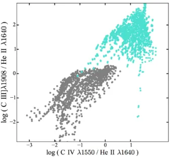
Jaskot and Ravindranath (2016) used different ESs (bpass) and studied the effect of shocks on SFGs using also cloudy. They found that Ciii]/Heii vs Civ/Heii separates star-forming regions from shock-ionized gas, and concluded that the Ciii] doublet, which is frequently observed in low-metallicity SFGs and which can be detectable for a wide range of low low-metallicity conditions, is a promising emission line for diagnostic and characterization of galaxies at high redshift.
1.5
Searching for the first galaxies
Most of the high-redshift galaxies candidates have been found through ultra deep observations using the different filters of the WFC3 (IR) on board of the Hubble Space Telescope (e.g. Ellis et al. (2013)) and through the Lyman Break technique (LBT, Giavalisco (2002) for a review about the topic).
In the LBT, the selection of the candidates is made by their photometric colours, considering the strong discontinuity on the rest-frame UV continuum due to the absorption by neutral hydrogen of the IGM. Galaxies with high UV luminosity are easier to detect.
The LBT allows to select thousands of high-redshift candidates at once, where the confirmation can be made with follow-up optical spectroscopy (z = 5 - 7). However, it is often common to detect just one emission line in the spectra of these galaxies: Lyα. Some exceptions are strong UV emission lines, such as Heii or Ciii] (e.g. Stark et al. (2015)).
The LBT technique has been extended to redshifts into the reionization epoch (e.g. Bouwens et al. (2011)), but around z ∼ 7, it is very difficult to obtain spectroscopic confirmation. These sources are observed on Earth at near-infrared wavelengths (which can be overcomed by using space telescopes). However, the main difficult is to recover the Lyα flux due to the amount of neutral hydrogen as we enter into the reionization epoch. Lyα is strongly scattered which suppresses a significant fraction of the total flux of the line.
The Lyα emission line then provides a probe of the condensation of primordial gas into the first galaxies. It is intrinsically the brightest UV emission line in the spectrum and it is commonly used to search for distant galaxies.
Progress have been made by searching for luminous Lyα emitters (LAE), which can be detected using surveys designed to spot these sources at specific redshifts (e.g. Matthee et al. (2015), Santos et al. (2016)) or using strong lensed galaxies (e.g. Stark et al. (2015), Stark et al. (2014)). Over the last years, the number of high-redshift galaxies at z ∼ 7 detected through their Lyα emission line has raised (e.g. Ouchi et al. (2009), Konno et al. (2014), Sobral et al. (2015), Matthee et al. (2017)), being brighter LAEs at the end of reionization epoch more common than previously thought (e.g. Santos et al. (2016)) and powered by strong ionizing sources (e.g. Matthee et al. (2017)).
Moreover, all high-redshift galaxies selected through other UV features show prominent Lyα line and an extremely hard radiation spectra. For example, some galaxies show Civλλ1548,1550 (e.g. Stark et al. (2015)), requiring the production of a large number of photons more energetic than 47.9 eV. The Civ emission line is associated with low luminosity narrow-line AGNs, but also has been found in dwarf galaxies at lower redshifts, probably powered by harder radiation fields associated with low metallicity stars (e.g. Vanzella et al. (2016)).
Several young galaxies, analogues of primeval galaxies, have been detected around z ∼ 2 - 3 (e.g. Amor´ın et al. (2017), Vanzella et al. (2016)). These galaxies exhibit the properties expected for high-redshift galaxies: they are compact star-forming, low-mass and low-metallicity systems, characterised by a strong UV spectra with bright emission lines, which indicates a hard radiation field produced by young and massive hot stars. Other possible analogues to high redshift systems are the “Green Peas”, low-mass and compact galaxies with very active star formation, found at even lower redshifts (see e.g. Izotov et al. (2016)).
1.6
Modelling emission from high-redshift galaxies
1.6.1 Photoionization Codes
Photoionization simulation codes calculate the physical conditions of a gas irradiated by an external source of ionization and predict the resulting spectrum.
The first codes were developed in the late 60’s with the aim of study low-density nebulae (e.g. Harrington (1968)). Several developments have been made since then, to include, for example improvements in the atomic processes, dealing with higher densities and higher photon energies and different optical depths. Codes can differ in their radiative treatment, geometry, equilibrium conditions, shocks treatment, atomic data, number of emission lines that can be treated, etc. Some examples of photoionization codes are cloudy (Ferland et al. (1998)), mappings-iii (Sutherland et al. (2013)), mocassin (Ercolano et al. (2003)), xstar (Kallman (1999)) and titan (Dumont et al. (2000)).
cloudy is an open source photoionization plasma simulation code, originally development in the late 70’s to simulate gas conditions on black hole accretion discs to study the broad-line regions of AGNs (e.g. Rees et al. (1989)). cloudy incorporates all the physics from the first principles (with a constant update of its microphysical processes) to determines the physical conditions within a non-equilibrium gas. Despite the great variety of existent objects, from stars, to galaxies or clusters of galaxies, usually the density is so low on these environments that the plasma is collisionless and is not in thermodynamic equilibrium. For that reason, cloudy has been widely used by the astronomical community to simulate condition of other objects such as galactic HII regions, Planetary Nebulae and SFGs.
cloudy solves the 1D radiative transfer equations to simulate complex physical environments. It determines the physical conditions of the gas by solving the equations of statistical equilibrium, charge conservation, and conservation of energy, taking into consideration the relative population in different levels (the microphysics processes of astronomical plasmas are of great importance to reach better accuracies towards interpreting astronomical quantities). As a result, it determines the level of ionization, the gas chemical state and kinetic temperature, as well as the particle density and the full spectrum, with hundreds to thousands of emission lines (Osterbrock and Ferland (2006)).
Codes such as mocassin can deal with more complex geometries computing for example 3D radiative transfer through Monte Carlo simulations. However, 1D codes allow faster computations (ideal for creating large grids of models) and are a good approximation to spatially unresolved objects when the exactly distribution of gas is not known (see Section 2.1.1 for a discussion about the gas geometry of high-redshift systems).
1.6.2 Evolutionary Synthesis models
Distant galaxies that hold unresolved stellar population are commonly described by their spectral energy distributions (SED), i.e. their energy as function of frequency or wavelength. Their analysis and understanding are on the basis of modern studies of galaxy formation and evolution, since the physical properties of the galaxies are encoded in their SEDs. They allow to estimate the properties of a galaxy such as its star formation history (SFH), stellar initial mass function (IMF), ionization
radiation field, total mass of stars, stellar metallicity, and the gas and dust contents.
Along with its interpretation through fitting techniques (first applied by Faber (1972)), synthetic SED models have been developed since the late 60’s (e.g. Tinsley (1968)), based on stellar evolution theory and/or empiric models. These synthetic SEDs are Evolutionary Synthesis (ES) models (Maraston (1998)), also refereed as Stellar Population Synthesis (SPS), where the SFH is computed based on an IMF. Some examples are starburst99 (Leitherer et al. (1999)), pegase (Fioc and Rocca-Volmerange (1999)), fsps (Conroy et al. (2009)) and ESs from Bruzual and Charlot (2003). ES models can be used to derive the physical properties of a galaxy, predicting the integrated emission of stellar populations, interpreting observations, besides helping to delineate observational strategies. They are complementary to fitting techniques, where a code fits an observed spectrum with a model adding spectral components from a pre-defined base spectra, which can include evolu-tionary synthesis models, observed templates and individual stars (e.g. starlight, Cid Fernandes et al. (2005)). Novel approaches using genetic differential evolution optimization along with several numeric techniques (e.g. artificial intelligence strategies for spectra library selection) have been recently developed, accomplishing better SFHs fitting (fado, Gomes and Papaderos (2017)). Synthetic spectra concept
On the basis of a synthetic spectra of a stellar population is a simple stellar population, with a particular metallicity and abundance pattern, that evolves in time. The creation of stellar popu-lations is based on isochrones, that specify the location of stars with the same age and metallicity on the Hertzsprung-Russel diagram; an IMF, which describes the initial mass distribution along the main sequence as function of metallicity; and stellar spectral libraries, that convert the stellar evolution results into readable SEDs. These are the building blocks of more complex systems. A review on ESs can be found in Conroy (2013).
The most updated models also include dust, which plays an important role obscuring the UV light, particularly important for SFGs with high metallicity. Another important feature is the neb-ular emission which comprises two components: a continuum emission from free-free, free-bound, and two-photon emission, and a recombination line emission, described in Section 1.3.4. Both com-ponents can be added to the SEDs as function of the physical state of the gas, using photoionization codes such as the ones mentioned in Section 1.6.1.
For SFGs, the UV flux is dominated by the light produced by young and hot stars and the sur-rounding ionized gas, which is responsible for nearly all the UV emission lines present in the spectra, therefore nebular emission is more important with high star formation rates, low metallicities and at younger ages, being very important for high-redshift galaxies (Schaerer and de Barros (2009)). BPASS
In stellar populations that have formed stars continuously over its lifetime, both young and old stars contribute for a “stable” UV SED, while young starbursts, which contain larger portions of hot massive stars emit more ionizing photons. This is particularly important for low metallicity systems, where binary and rotation effects are more important, resulting in a modified ionizing spectra (Eldridge et al. (2008), Stanway et al. (2014)).
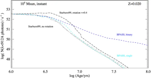
bpass is the Binary Population And Spectral Synthesis code 1 (Eldridge and Stanway (2009)), that uses theoretical stellar evolution models combined with synthetic stellar atmospheres and include binary and rotation effects. Binary interactions create more hot helium and Wolf-Rayet stars due to the removal of the hydrogen envelope in primary stars. This enhances mass-losses, originating harder ionizing photons at later times than single star populations. Binaries also allow mass transfer to secondary stars increasing their mass and revitalization, and can lead to binary mergers producing single massive stars (Eldridge et al. (2008)). As a consequence it results in a top heavy mass function and more massive stars at later stages than expected, which increases the ionizing flux at later times (& 10 Myrs, Stanway et al. (2016), Figure 1.7).
Figure 1.7: bpass single and binary evolutionary pathways for an instantaneous star formation history, at∼ 1.4 solar metallicity, and starburst99 with both a rotation parameter v = 0.4 and no rotation, for comparison. Note that the binary effects are even more important at sub-solar metallicities. From Stanway et al. (2016).
Rotation creates hotter stars and extends the star lifetime (Yoon and Langer (2005)). Rotation can result in stellar layer mixing, allowing high hydrogen burning (e.g. de Mink et al. (2013)). This effect is particularly important for high-mass stars (≥ 20 M ) and low metallicities (e.g. Eldridge
et al. (2011)), where stellar winds are not strong enough to make these stars spin down and so they can remain rotating over their main sequence lifetime in a quasi-homogeneous evolution (QHE). This increases the SED flux at all ages.
When studying high-redshift galaxies, it is therefore necessary to use an ES that includes binaries and rotation effects, which can reproduce better the stellar populations of these galaxies.
1.7
Motivation and Goals
There is not a universal definition for “first galaxy” (Bromm and Yoshida (2011)). Observations and theories have been developed side by side to understand the formation and evolution of the first galaxies. For that reason, this work is based on the knowledge obtained from many observations but also from the physical concepts that are needed to build a “first galaxy”.
The first galaxies are expected to be powered by strong ionizing sources where the formation and evolution of massive stars have a major impact. These are also the most likely sources responsible for the reionization of the Universe.
The rest-frame UV of high-redshift galaxies show emission lines characteristic of massive stars, such as Heiiλ1640 ˚A and Ciii]λλ1907,1910 ˚A (e.g. Masters et al. (2014), Steidel et al. (2016), Stark et al. (2014)), indicative of a hard ionizing radiation field. These characteristics are more common in high-redshift galaxies than in the local ones. However, several analogues of high-redshift galaxies have been found at z ∼ 2 - 3, with high star formation rates and similar emission properties (e.g. Amor´ın et al. (2017)). These galaxies present low metallicity, indicating that they host predomi-nantly POP III stars. Their study can help on the understanding of higher redshift systems and to establish whether the high-ionization emission of these sources is powered by SFG hosting hot and low-metallicity stars or AGNs, since both can potentially provide high energy photons. For “typical galaxies” at lower redshifts, such tools already exist using rest-frame optical emission line-ratios (e.g. BPT diagram). Diagnosis tools for the rest-frame UV emission lines, that take into consideration the properties of primeval galaxies, have just began to be developed using photoionization codes (e.g. Feltre et al. (2016), Gutkin et al. (2016)).
At high redshift, galaxies are unresolved and the emission we observe is the integrated light of different stellar populations (probably with different ages and metallicities). Their interpretation and comparison with the data request the use of an Evolutionary Synthesis (ES) code, which is based on known parameters, such as the initial mass function, metallicity and star formation history. Commonly, evolutionary synthesis codes differ from codes based on empirical observations of nearby stellar populations to theoretical stellar and atmosphere models. However, conventional ESs have shown not to be sufficient to explain the emission line strengths that have been detected in star forming galaxies with characteristics of primeval systems (e.g. Steidel et al. (2016)). Conventional ESs, such as starburst99, lack on extensive details of massive star populations and the strengths of the lines are difficult to reproduce with these models (Shapley et al. (2003)). ESs that include binary stars and rotation effects, as well as low metallicities, are then needed to explain the strengths of these lines at high-redshift (e.g. Eldridge and Stanway (2012), Steidel et al. (2016)). Moreover, ESs which include binaries and rotation are essential to understand the reionization history, since they can explain the “missing photons” necessary for the reionization (Ma et al. (2016)).
In this work we use the photoionization plasma simulation code cloudy 13.03, last described in Ferland et al. (2013), to simulate the gas conditions in high-redshift galaxies and to predict the emission line spectra of these low density, almost dust-free and low-metallicity systems.
We compute a grid of models to simulate star forming galaxies using both a black body shape (which does not suffers the limitations introduced by the approximations and lack of accuracy of stellar models) and the bpass v2.0 ESs. To understand low metallicity, high-redshift SFGs, it is necessary to take into account massive stellar evolution and its interpretation. bpass uses theoretical state-of-the-art stellar evolution models combined with synthetic stellar atmospheres that include binary and rotation effects. Binary evolution extends the lifetime of stars, increasing the influence of very blue stars in the spectra.
Including the effects of massive stars is also important to understand the nature high-redshift galaxies, such as CR7 (Sobral et al. (2015)), selected through its strong Lyα emission line, presenting
also Heii. The absence of other emission lines suggests a metal-free POP III stellar population. Stellar evolution models can help to address the nature of these galaxies (Bowler et al. (2016)).
We also create models to simulate nebular emission from AGNs using a power-law shape. The presence of supermassive black holes at high redshift create powerful AGNs that present hard ionizing spectra and are difficult to distinguish from SFGs with such characteristics.
The key goal of this work is to derive the signatures of the first galaxies using UV emission line-ratios, helping on the understanding of the nature of these sources and make observational predictions for upcoming telescopes, such as the James Webb Space Telescope. At high redshift the total flux of the Lyα emission line is attenuated by the intergalactic medium, being necessary to study the behaviour of other UV emission lines that allow to understand these high-redshift systems.
In Chapter 2 we describe our SFGs and AGNs cloudy models in detail and in Chapter 3 we present the main differences between our models, as well as our modelling results using UV line-ratios to explore the characteristics of both ionizing sources.
In Chapter 4 we analyse analogues of primeval galaxies around the peak of star formation of the Universe (e.g. Sobral et al. (2014)). We derive the physical properties of young SFGs from Amor´ın et al. (2017) and bright Lyα emitters from Sobral et al. (in prep). We also present observational interpretation of high-redshift galaxies expected to be observed with future telescopes such as the James Webb Space Telescope. We then extend our modelling results to galaxies at higher redshift, where we used our cloudy models to study the Lyα escape fraction in galaxies at z ∼ 6 - 7 (presented in Matthee et al. (2017)).
In Chapter 5 we present our study of galaxies from the HiZELS (High-z Emission line survey), which we fully analyse, and select two SFGs at z ∼ 1.5 to apply our modelling results.
Chapter 2
cloudy photoionization modelling
To perform photoionization simulations, the physical properties of the gas and the external source of radiation need to be specified.
A general description of the properties of the gas cloud used in this study is presented in Section 2.1. In Section 2.2 we describe other parameters and commands common to all models. The external radiation field that strikes the cloud (i.e. the incident radiation field) is described in Section 2.3.
2.1
The gas cloud
To perform accurate radiative transfer simulations, cloudy needs information about the envi-ronment where the light of the ionizing source is passing through. The main parameters that must be specified to simulate the gas cloud are the geometry of the gas, the gas density, its chemical content and its grain content.
2.1.1 Geometry of the gas cloud
cloudy has two geometry limiting cases: an open geometry (plane-parallel) and a closed geom-etry (spherical). In an open geomgeom-etry the diffuse emission from the illuminated face of the cloud escapes from the system without striking other clouds, whereas in a closed geometry the emission from the illuminated face of the cloud strikes the gas on the opposite side of the cloud (Figure 2.1).
Figure 2.1: cloudy gas geometries (both one-dimensional) as illustrated in the documentation of cloudy last de-scribed in Ferland et al. (2013).
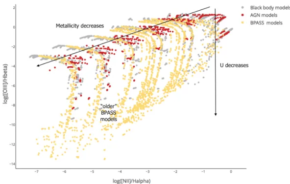

![Figure 3.7: Log(C iii ]λ1909/He ii λ1640) vs log(C iv λ1549/He ii λ1640) diagram spanning the full range of parameters listed in Table 3.1.](https://thumb-eu.123doks.com/thumbv2/123dok_br/15198522.1017739/57.918.165.749.419.786/figure-log-diagram-spanning-range-parameters-listed-table.webp)