Desagregação de chuvas diárias para o estado do Tocantins, Brasil

(1)

www.ambi-agua.net E-mail: ambi.agua@gmail.com

Rev. Ambient. Água vol. 12 n. 4 Taubaté – Jul. / Aug. 2017

Daily rainfall disaggregation for Tocantins State, Brazil

doi:10.4136/ambi-agua.2077

Received: 10 Jan. 2017; Accepted: 08 May 2017

Virgilio Lourenço da Silva Neto1*_{; Marcelo Ribeiro Viola}2_; Demetrius David da Silva3_{; Carlos Rogério de Mello}2_;

Silvio Bueno Pereira3_{; Marcos Giongo}4

1_{Instituto Federal de Educação, Ciência e Tecnologia do Tocantins (IFTO), Dianópolis, TO, Brasil} 2_{Universidade Federal de Lavras (UFLA), Lavras, MG, Brasil}

Departamento de Engenharia de Água e Solo

3_{Universidade Federal de Viçosa (UFV), Viçosa, MG, Brasil}

Departamento de Engenharia Agrícola

4_{Universidade Federal do Tocantins (UFT), Gurupi, Tocantins, Brasil}

Programa de Pós-Graduação em Ciências Florestais e Ambientais

*_{Corresponding author: e-mail:}_{virgilio.neto@ifto.edu.br,}

marcelo.viola@deg.ufla.br, demetrius.ufv@gmail.com, crmello@deg.ufla.br, silviopereira.ufv@gmail.com, giongo@uft.edu.br

ABSTRACT

In order to design effective Brazilian hydraulic structures, it is necessary to obtain data relating to short-duration intense rainfall from historical series of daily rainfall. This recurring need can be fulfilled by rainfall disaggregation methodology. The objective of this study was to determine the intense rainfall disaggregation constants for the State of Tocantins and to compare these constants with those obtained for other regions of Brazil. For the modeling of the frequency of intense rainfall of different durations of less than 24 hours, the Gumbel probability distribution (GPD) was employed using rainfall series from 10 locations in Tocantins state. The results showed that the GPD was adequate by the Kolmogorov-Smirnov and Chi-square tests. The disaggregation constants presented low variability values for different return periods (from 10 to 100 years); the values for Tocantins state are: h12h/h24h=0.93, h6h/h24h=0.86, h4h/h24h=0.82, h3h/h24h=0.78, h2h/h24h=0.72, h1h/h24h=0.61, h50min/h1h=0.92, h40min/h1h=0.83, h30min/h1h=0.68, h20min/h30min=0.76 e h10min/h30min=0.46. The comparison of the results with those from studies developed for other Brazilian regions showed variations of up to -62.30%, allowing us to conclude that the use of local constants is important in the process of rainfall disaggregation.

Keywords: hydrology, precipitation, short-duration intense rainfall.

Desagregação de chuvas diárias para o estado do Tocantins, Brasil

RESUMO

(2)

Objetivou-Rev. Ambient. Água vol. 12 n. 4 Taubaté – Jul. / Aug. 2017

se neste trabalho determinar constantes de desagregação de chuvas intensas para o Estado do Tocantins e proceder a comparação destas constantes com aquelas obtidas para outras regiões do Brasil. Para a modelagem da frequência das chuvas intensas de diferentes durações, foi empregada a distribuição de probabilidades Gumbel, tendo sido utilizadas séries pluviográficas de 10 localidades do estado do Tocantins. Os resultados mostraram que a distribuição de probabilidades Gumbel foi considerada adequada pelos testes Kolmogorov-Smirnov e Qui-quadrado. Observou-se que as constantes de desagregação apresentaram valores praticamente invariáveis para tempos de retorno entre 10 e 100 anos, tendo sido obtidas as seguintes constantes médias para o estado do Tocantins: h12h/h24h=0,93, h6h/h24h=0,86, h4h/h24h=0,82, h3h/h24h=0,78, h2h/h24h=0,72, h1h/h24h=0,61, h50min/h1h=0,92, h40min/h1h=0,83, h30min/h1h=0,68, h20min/h30min=0,76 e h10min/h30min=0,46. A comparação dos resultados com os de estudos desenvolvidos para outras regiões brasileiras mostrou variações de até -62,30%, permitindo se concluir que a utilização de constantes locais é importante no procedimento de desagregação de chuvas.

Palavras-chave: chuvas intensas de curta duração, hidrologia, precipitação.

1 .

INTRODUCTION

In the planning and management of soil and water resources, it is indispensable to have backgrounds related to the climatic variables, among which heavy rainfall may be highlighted (Souza et al., 2012). However, according to Back (2009), there are some significant problems in obtaining the intensity-duration-frequency relation (IDF) of heavy rainfall with lower durations (< 24 hours) due to the scarcity of rainfall records and to the short-term observed periods.

According to Cardoso et al. (1998) and Oliveira et al. (2000), in order to overcome these problems, it is necessary to estimate short-duration heavy rainfall from daily rainfall records, since the latter are much more available in the Brazilian territory. According to Engida and Esteves (2011), Gyasi-Agyei (2005), Paola et al. (2014) and Yusop et al. (2014), an alternative to circumvent this data limitation is the application of the rainfall disaggregation methodology, which allows the estimation of short-duration heavy rainfall from the annual maximum daily rainfall (hday) monitored by standard rain gauges. In this methodology, the 24-hour intense

rainfall (h24h) is initially estimated from hday, as the difference between them relates to the fact

that the latter corresponds to the depth observed based on a fixed interval of 24 hours, since the readings are performed daily at the same time (normally 0900 every day), while h24h relates to

precipitation monitored during any 24-hour period by means of pluviographs, without fixing the beginning of the initial time (Mello et al., 2001).

For Brazil, there are a few studies related to rainfall disaggregation coefficients determination for a given region (or state). However, it is possible to highlight the studies of Taborga (1974) and CETESB (1980). Both estimated average coefficients for Brazil, Back et al. (2012) for Santa Catarina, Teixeira et al. (2011) for Pelotas and ATP-Engenharia e INFRAERO (2010) for Manaus. Many Brazilian states lack detailed studies regarding rainfall disaggregation coefficients, especially for the states of the Northern Brazilian region. Because of this, the pioneer study of CETESB (1980) is still used as a reference for heavy rainfall studies (Silveira, 2000; Mesquita et al., 2009; Garcia et al., 2011; Teodoro et al., 2014).

According to this study, there is a virtually invariant relationship between h24h and hday

(h24h / hday), which can be assumed to be equal to 1.14, which means that, on average, h24 is

14% higher than hday. Another important aspect of the CETESB (1980) study is the availability

(3)

an important investigation not yet carried out is the analysis of quantitatively possible errors associated with short-duration heavy rainfall proportioned by disaggregation coefficients generated for a large and heterogeneous region applied to another region which is smaller and has a specific climate. The application of coefficients generated by CETESB (1980) to estimate heavy rainfall in a specific state is a good example of this.

Tocantins State occupies about 277,620 km2_{and is located in the northern region of Brazil.}

In the last decades, Tocantins has experienced an intense expansion of agricultural and livestock activities as well as increased population pressure which require scientific investigations to guide its orderly development. Considering the agricultural potential of this state and the damaging effects of the high kinetic energy of heavy rains in rural environments, such knowledge is essential to support soil and water conservation studies. Consideration should also be given to the growth of the State and the need for background data for the design of hydraulic structures such as urban and rural drainage systems and landfills, among others.

In this context, the objective of this study was to determine the intense rainfall disaggregation constants for the Tocantins State from an historical series of 10 rain gauge stations, to analyze the influence of the frequency of the hydrological variable on the values of the disaggregation constants and the acquisition of the following relationships for the State of Tocantins: h12h/h24h, h6h/h24h, h4h/h24h, h3h/h24h, h2h/h24h, h1h/h24h, h50min/h1h, h40min/h1h, h30min/h1h,

h20min/h30min and h10min/h30min. Specifically, the objective of this study was to verify whether the

average disaggregation constants available for Brazil or available for other Brazilian states are adequate for estimating short-duration heavy rainfall for Tocantins State.

2. MATERIAL AND METHODS

The State of Tocantins is located between parallels 5º10'06" and 13º27'59" south latitude and meridians 45º44'46"and 50º44'33" west longitude, with an area of 277,621 km², representing 3.26% of the total area of Brazil and 7.2% of the northern region. The Amazon biome, characterized by seasonal, open and dense Ombrophylous forests, occupies 9% of the state, while the predominant biome in 91% of the state is the Cerrado, characterized by vegetation formations of savanna and forest structure (IBGE, 2004; Tocantins, 2012).

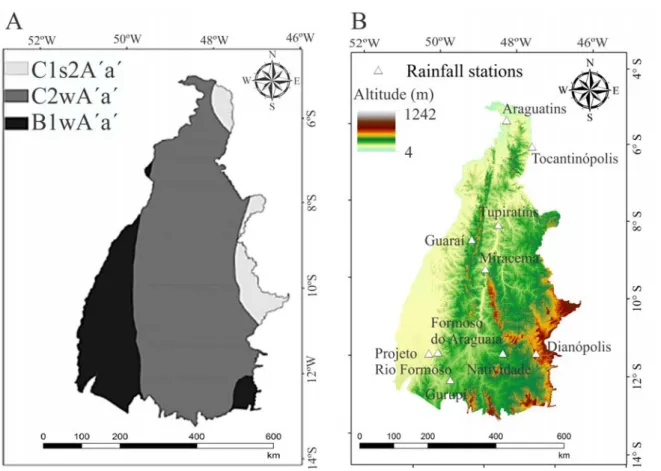
According to Souza (2016) in Tocantins there are three homogeneous climatic regions, according to the Thornthwaite classification (Figure 1): a) C1s2A’a’- dry sub-humid climate, with high amount excess rain in the summer, mega-thermal; (b) C2wA’a’- sub-humid climate, with moderate water deficiency in the winter, mega-thermal; and c) B1wA’a’ - humid climate, with moderate water deficiency in the winter, mega-thermal.

The database used in this study consisted of an historical series of maximum rainfall intensities associated with the durations of 10, 20, 30, 40, 50, 60, 120, 240, 360, 720 and 1440 minutes for 10 rain-gauges, located in the Tocantins State, within the hydro-meteorological network of the Brazilian National Water Agency (ANA), that present pluviographic recordings from 1989 to 1999. Intense rainfall data were acquired for each station. First, the most intense rainfall events were identified for each year. Second, the maximum rain depth for each evaluated rainfall duration and respective average maximum intensity were calculated, according to Silva et al. (2003).

(4)

Figure 1. Thornthwaite and Matter climatic classification for the Tocantins State (Souza, 2016) (A); ASTER digital elevation model for the Tocantins State and spatial distribution of the rainfall stations used in the present study (B).

The Gumbel Probability Distribution (GPD) was adjusted to model the frequency of heavy rainfall of different durations in the Tocantins. This distribution has been widely applied to intense rainfall series as these datasets present an asymptotic frequency behavior, with a positive tail. Good results can be highlighted by GPD application as those obtained in the studies of Waylen and Woo (1982), Cardoso et al. (1998), Mello et al. (2001), Coles et al. (2003), Campos et al. (2015), Ferreira et al. (2005), Oliveira et al. (2005), Back (2006), Silva et al. (2003), Damé et al. (2006), Back (2009), Damé et al. (2010), Villarini et al. (2011), Back et al. (2012), Mello and Viola (2013), Borges and Thebaldi (2016) and Caldeira et al. (2015). GPD can be described by Equation 1 (Mello and Silva, 2013).

. . . ₍₁₎

where:

x is the hydrological variable, α is the scale parameter, and

μ is the position parameter of the distribution.

(5)

, ₍₂₎

0,45 ∙ (3)

where:

and s are the mean and standard deviation of the historical series, respectively.

The integration of Equation 1 provides the cumulative probability function (CPF) (Equation 4).

P X x 1 e ∝. (4)

The suitability of the GPD was verified by the Kolmogorov-Smirnov and Chi-square tests at a significance level of 5%. The estimation of the hydrological variable associated with a given recurrence (XTR) was obtained by Equation 5.

(5)

where:

TR is the return period, in years.

For the determination of the disaggregation coefficients, the following TR values were considered: 2, 5, 10, 20, 50 and 100 years. Subsequently, for each frequency analyzed, the duration-to-date relationship method was used to obtain the disaggregation constants. According to Tucci (2009), this method considers two aspects: a) the tendency of the probability curves of different durations to remain parallel to each other; and b) for different locations there is a great similarity in the relationships among average maximum precipitations varying according to different durations. The relationships among different durations were obtained according to Equation 6.

/ (6)

where:

/ , is the constant that characterizes the relation between the intense rains of duration t1 and of duration t2.

The following disagregation coefficients were calculated: h12h/h24h, h6h/h24h, h4h/h24h,

h3h/h24h, h2h/h24h, h1h/h24h, h50min/h1h, h40min/h1h, h30min/h1h, h20min/h30min and h10min/h30min for all

evaluated return periods. Because the database of the present study does not have the series of annual maximum daily precipitation (hday) for the 10 locations used in this study, it was not

possible to obtain the h24h/hday ratio. However, this is not characterized as a limitation for the

application of the constants developed herein, since according to CETESB (1980), the h24h/hday

ratio presents a quasi-constant value of 1.14.

3. RESULTS AND DISCUSSION

(6)

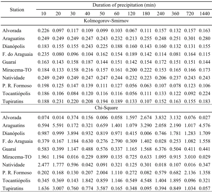
statistically null value of the Kolmogorov-Smirnov test for the studied series is 0.391 (ΔFTab(11;0.05)), all the 120 adjustments were approved at a 5% probability level. However, based

on Chi-Square test, for which the null value for the studied series is 3.845 (λ²Tab(1;0.05)), 5

adjustments were approved only when 1% probability level was considered: 20- and 1440-min for Araguatins, 30-min for Dianópolis, 240-min for Guaraí and 180-min for Tocantinópolis. Despite of these 5 exceptions, taking the results into account, we can affirm that GPD was adequate for this study.

Table 1. Maximum adjustment error of the Gumbel distribution aiming towards application of the Kolmogorov-Smirnov and Chi-square tests for the maximum rainfall series with durations between 10 and 1440 minutes for 10 locations in the Tocantins State.

Station Duration of precipitation (min)

10 20 30 40 50 60 120 180 240 360 720 1440 Kolmogorov-Smirnov

Alvorada 0.226 0.097 0.117 0.109 0.099 0.103 0.067 0.111 0.157 0.132 0.157 0.163 Araguatins 0.249 0.249 0.249 0.247 0.243 0.232 0.213 0.255 0.248 0.251 0.301 0.280 Dianópolis 0.183 0.155 0.155 0.243 0.225 0.188 0.160 0.143 0.160 0.132 0.131 0.155 F. do Araguaia 0.235 0.080 0.096 0.104 0.162 0.154 0.189 0.142 0.114 0.081 0.164 0.115 Guaraí 0.163 0.143 0.158 0.187 0.144 0.151 0.142 0.154 0.172 0.151 0.151 0.144 Miracema-TO 0.184 0.133 0.158 0.216 0.157 0.161 0.200 0.222 0.153 0.165 0.166 0.173 Natividade 0.249 0.249 0.249 0.247 0.247 0.244 0.232 0.223 0.206 0.237 0.243 0.243 P. R. Formoso 0.198 0.125 0.147 0.139 0.111 0.127 0.056 0.063 0.107 0.078 0.123 0.106 Tocantiópolis 0.186 0.106 0.084 0.120 0.116 0.116 0.056 0.111 0.133 0.122 0.092 0.224 Tupiratins 0.188 0.231 0.220 0.208 0.194 0.189 0.133 0.107 0.152 0.163 0.155 0.183

Chi-Square

Alvorada 0.074 0.014 0.374 0.156 0.006 0.058 1.597 2.674 3.832 3.132 0.076 0.027 Araguatins 0.594 5.591 0.172 0.321 0.659 1.401 1.079 3.290 2.058 2.190 1.017 4.576 Dianópolis 0.987 0.999 3.894 0.932 0.819 0.971 0.415 0.006 0.746 1.781 1.283 1.709 F. do Araguaia 0.379 0.167 1.184 0.630 0.276 2.790 0.309 1.402 0.028 0.253 1.082 1.558 Guaraí 0.583 0.399 1.147 0.488 0.576 0.337 1.165 1.568 6.376 0.504 0.411 0.441 Miracema-TO 1.961 1.194 0.016 0.229 0.899 0.135 0.725 0.633 1.095 0.915 3.010 0.029 Natividade 2.477 1.777 0.596 0.042 0.091 0.321 0.125 0.301 0.018 0.107 0.016 0.347 P. R. Formoso 0.202 0.168 0.130 0.207 2.004 1.110 0.272 0.082 0.579 0.682 2.136 1.358 Tocantiópolis 0.345 0.369 0.143 1.842 0.859 1.146 0.549 4.548 1.404 1.895 0.096 0.321 Tupiratins 1.636 3.007 0.760 0.774 3.587 0.165 0.348 0.095 0.394 0.849 1.034 0.057

Figure 2 shows the disaggregation coefficients of rainfall as a function of the return period. There are differences in the values of the constants for the different locations studied, highlighting the lowest values of the constants h12h/h24h, h6h/h24h and h4h/h24h for Tupiratins.

(7)

(8)

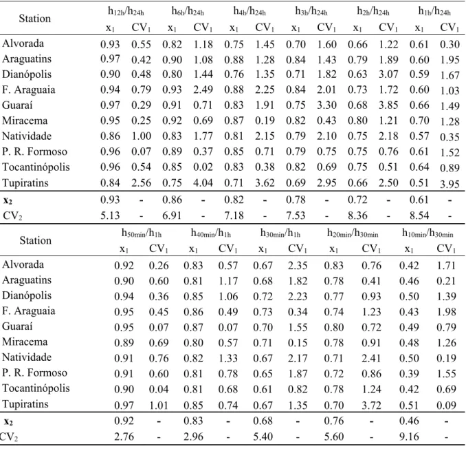
Table 2 presents the mean (x1) and coefficient of variation (CV1) for the intense rainfall

disaggregation coefficients for return periods from 10 to 100 years, for each of the 10 pluviographic stations employed. CV1 values are lower than 4.04% in all situations, indicating

that there is a reduced variation of the values of the coefficients for return periods between 10 and 100 years. Table 2 also presents the mean values (x2) of the disaggregation coefficients for

Tocantins State and respective coefficients of variation (CV2). These values correspond to the

mean and coefficient of variation for the set of 10 rainfall stations used for each coefficient. In this situation, the reduced variation of the disaggregation coefficients in the Tocantins State can also be highlighted, which means that they can be applied for estimating heavy rainfall with durations of less than 24 hours in Tocantins State.

Another relevant aspect when analyzing the disaggregation coefficients is their non-linear characteristic. It can be observed, for example, that, on average, the 12-hour heavy rainfall equals 93% of the 24-hour depth, or even the intense 10-minute rainfall equals 46% of the 30-minute rainfall.

Table 2. Mean (x1) and coefficient of variation (CV1) of the disaggregation coefficients for return period times varying between 10 and 100 years for each studied station, and mean (x2) and coefficient of variation (CV2) for each constant in Tocantins State.

Station h12h/h24h h6h/h24h h4h/h24h h3h/h24h h2h/h24h h1h/h24h x1 CV1 x1 CV1 x1 CV1 x1 CV1 x1 CV1 x1 CV1 Alvorada 0.93 0.55 0.82 1.18 0.75 1.45 0.70 1.60 0.66 1.22 0.61 0.30 Araguatins 0.97 0.42 0.90 1.08 0.88 1.28 0.84 1.43 0.79 1.89 0.60 1.95 Dianópolis 0.90 0.48 0.80 1.44 0.76 1.35 0.71 1.82 0.63 3.07 0.59 1.67 F. Araguaia 0.94 0.79 0.93 2.49 0.88 2.25 0.84 2.01 0.73 1.72 0.60 1.03 Guaraí 0.97 0.29 0.91 0.71 0.83 1.91 0.75 3.30 0.68 3.85 0.66 1.49 Miracema 0.95 0.25 0.92 0.69 0.87 0.19 0.82 0.43 0.80 1.21 0.70 1.28 Natividade 0.86 1.00 0.83 1.77 0.81 2.15 0.79 2.10 0.75 2.18 0.57 0.35 P. R. Formoso 0.96 0.07 0.89 0.37 0.85 0.71 0.79 0.75 0.75 0.76 0.61 1.52 Tocantinópolis 0.96 0.54 0.85 0.02 0.83 0.38 0.82 0.69 0.75 0.51 0.64 0.89 Tupiratins 0.84 2.56 0.75 4.04 0.71 3.62 0.69 2.95 0.66 2.50 0.51 3.95

x2 0.93 - 0.86 - 0.82 - 0.78 - 0.72 - 0.61 - CV2 5.13 - 6.91 - 7.18 - 7.53 - 8.36 - 8.54 - Station _x1h50min/h1h _CV1 _x1h40min/h1h _CV1 _x1h30min/h1h _CV1 h20min/h30min _x1 _CV1 h10min/h30min _x1 _CV1 Alvorada 0.92 0.26 0.83 0.57 0.67 2.35 0.83 0.76 0.42 1.71 Araguatins 0.90 0.60 0.81 1.17 0.68 1.82 0.78 0.41 0.46 0.21 Dianópolis 0.94 0.36 0.85 1.06 0.72 2.23 0.77 0.93 0.50 1.39 F. Araguaia 0.95 0.45 0.86 0.49 0.73 0.34 0.74 1.23 0.43 1.98 Guaraí 0.95 0.07 0.87 0.07 0.70 1.55 0.80 0.72 0.49 0.79 Miracema 0.89 0.69 0.80 0.57 0.71 0.15 0.78 0.91 0.48 1.26 Natividade 0.91 0.76 0.82 1.33 0.67 2.17 0.71 2.41 0.50 0.19 P. R. Formoso 0.91 0.60 0.81 0.78 0.65 1.87 0.72 0.86 0.39 1.55 Tocantinópolis 0.90 0.04 0.81 0.68 0.61 0.82 0.78 1.24 0.42 0.69 Tupiratins 0.97 1.01 0.85 0.74 0.67 1.35 0.70 3.72 0.51 0.09

x2 0.92 - 0.83 - 0.68 - 0.76 - 0.46 -

(9)

The comparison of the mean disaggregation coefficients obtained in the present study (x2, Table 2) with the results of CETESB (1980) for Brazil, Back et al. (2012) for the Santa

Catarina coast, Teixeira et al. (2011) for Pelotas and ATP-Engenharia / INFRAERO (2010) for Manaus, is presented in Table 3.

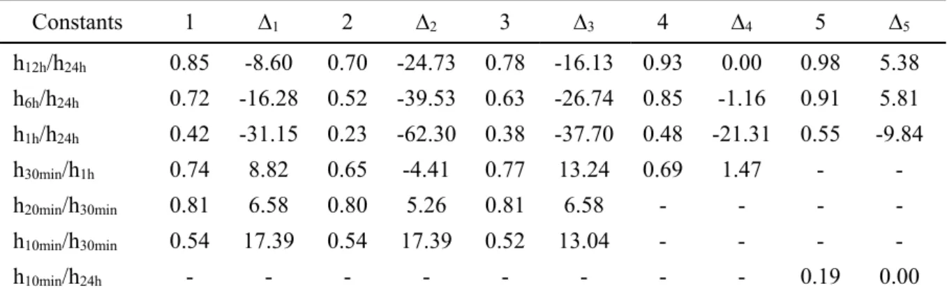
Table 3. Some disaggregation coefficients of intense rainfall obtained for Brazil (C1) (CETESB, 1980), Santa Catarina coast (C2) (Back et al., 2012), interior of Santa Catarina (C3) (Back et al., 2012), Pelotas (C4) (Teixeira et al., 2011) and Manaus (C5) (ATP-Engenharia/INFRAERO, 2010), and the respective variation percentage (Δ) in relation to the constants obtained for Tocantins State in the present study.

Constants 1 ∆1 2 ∆2 3 ∆3 4 ∆4 5 ∆5

h12h/h24h 0.85 -8.60 0.70 -24.73 0.78 -16.13 0.93 0.00 0.98 5.38 h6h/h24h 0.72 -16.28 0.52 -39.53 0.63 -26.74 0.85 -1.16 0.91 5.81 h1h/h24h 0.42 -31.15 0.23 -62.30 0.38 -37.70 0.48 -21.31 0.55 -9.84 h30min/h1h 0.74 8.82 0.65 -4.41 0.77 13.24 0.69 1.47 - - h20min/h30min 0.81 6.58 0.80 5.26 0.81 6.58 - - - - h10min/h30min 0.54 17.39 0.54 17.39 0.52 13.04 - - - -

h10min/h24h - - - 0.19 0.00

Comparing the coefficients obtained for Tocantins with those obtained by CETESB (1980) for Brazil as a whole, differences of up to -31.15% (h1h/h24h) are observed. For this particular

coefficient, for Tocantins the rainfall of 1h equals 61% of the rainfall of 24h, while the value available for Brazil (CETESB, 1980) is 42%. Analyzing the variations obtained in relation to Santa Catarina and Pelotas, greater differences are observed, with a variation that exceeds 60%. Manaus presents the smallest differences (up to -9.84%), which can be justified by the similarity of the predominant precipitation mechanism, which is majority convective rainfall (Reboita et al., 2010; Viola et al., 2014). When considering the 10-minute rainfall estimate of the 24-hour rainfall, it is observed that the sequential application of the constants h1h/h24h, h30min/h1h and

h10min/h30min results in a value of 0.19 (present study), 0.17 (Brasil, CETESB, 1980), 0.08 (Santa

Catarina coast, Back et al., 2012), 0.15 (outback Santa Catarina, Back et al., 2012) and 0.05 (Pelotas, Teixeira et al., 2011). Comparing this result to that of Manaus, we can observe the same value (0.19). This result agrees with Back's contention that the methodology of intense rainfall disaggregation has regional validity.

These results show significant differences among the disaggregation coefficients of the northern region (Manaus and Tocantins), southern Brazil (Pelotas, coast and Santa Catarina’s outback) and mean coefficient values for entire the country. Thus, it is important to emphasize the recommendations of Back et al. (2012) and CETESB (1980) that is more appropriate to use specific disaggregation coefficients for each site of interest as they present specific climatic factors that can directly affect the temporal behavior of this hydrological variable (short-duration heavy rainfall).

(10)

4. CONCLUSIONS

The GPD was adequate based on the Kolmogorov-Smirnov and Chi-square tests to model the frequency of occurrence of intense rainfall with durations of 10 to 1440 minutes of the 10 pluviographic stations of the Tocantins State addressed in the present study.

Disaggregation coefficients are quasi-constant for return periods between 10 and 100 years, which can be concluded based on the reduced coefficient of variation, which was lower than 4.04% in all analyzed situations.

The calculation of mean disaggregation coefficients indicated a coefficient of variation lower than 9.16% for all of them, which allows us to infer that the calculated average values are adequate for the disaggregation of heavy rainfall in Tocantins State.

Comparing the disaggregation coefficients estimated for Tocantins State in this study with others estimated for all of Brazil, as well as with those estimated by other stations/regions with different weather characteristics, differences of up to 60% were obtained.

5. REFERENCES

ATP ENGENHARIA; INFRAERO. Projeto de drenagem do Aeroporto Internacional Eduardo Gomes. Manaus, 2010. 59 p.

BACK, A. Relações intensidade-duração-frequência de chuvas intensas de Chapecó, Estado de Santa Catarina. Acta Scientiarum. Agronomy, v. 28, n. 4, p. 575-581, 2006.

BACK, A. Relações entre precipitações intensas de diferentes durações ocorridas no município de Urussanga, SC. Revista Brasileira de Engenharia Agrícola e Ambiental, v. 13, n. 2, p. 170-175, 2009. http://dx.doi.org/10.1590/S1415-43662009000200010

BACK, Á. J.; OLIVEIRA, J. L. R.; HENN, A. Relações entre precipitações intensas de diferentes durações para desagregação da chuva diária em Santa Catarina. Revista Brasileira de Engenharia Agrícola e Ambiental, v. 16, n. 4, p. 391-398, 2012. http://dx.doi.org/10.1590/S1415-43662012000400009

BORGES, G. M. R.; THEBALDI, M. S. Estimativa da precipitação máxima diária anual e equação de chuvas intensas para o município de Formiga, MG, Brasil. Revista Ambiente & Água, v. 11, n. 4, p. 891-902, 2016. http://dx.doi.org/10.4136/ambi-agua.1823 CALDEIRA, T. L.; BESKOW, S.; MELLO, C. R. D.; VARGAS, M. M.; GUEDES, H. A. S.

et al. Daily rainfall disaggregation: an analysis for the Rio Grande do Sul state. Revista Scientia Agraria, v. 16, n. 3, p. 1-21, 2015. http://dx.doi.org/10.5380/rsa.v16i3

CAMPOS, A. R.; SANTOS, G. G.; DOS ANJOS, J. C. R.; ZAMBONI, D. C. S.; MORAES, J. M. F. Equações de intensidade de chuvas para o Estado do Maranhão. Revista Engenharia na Agricultura, v. 23, n. 5, p. 435, 2015.

(11)

COLES, S.; PERICCHI, L. R.; SISSON, S. A fully probabilistic approach to extreme rainfall modeling. Journal of Hydrology, v. 273, n. 1, p. 35-50, 2003. https://doi.org/10.1016/S0022-1694(02)00353-0

COMPANHIA AMBIENTAL DO ESTADO DE SÃO PAULO - CETESB. Drenagem Urbana: manual de projetos. São Paulo: DAEE/CETESB, 1980. 466 p.

DAMÉ, R.; PEDROTTI, C.; CARDOSO, M.; SILVEIRA, C.; DUARTE, L. et al. Comparação entre curvas intensidade-duração-frequência de ocorrência de precipitação obtidas a partir de dados pluviográficos com aquelas estimadas por técnicas de desagregação de chuva diária. Revista Brasileira de Agrociência, v. 12, n. 4, p. 505-509, 2006.

DAMÉ, R. D. C.; TEIXEIRA, C. F.; TERRA, V. S.; ROSSKOFF, J. L. Hidrograma de projeto em função da metodologia utilizada na obtenção da precipitação. Revista Brasileira de Engenharia Agrícola e Ambiental, v. 14, n. 1, p. 46-54, 2010. http://dx.doi.org/10.1590/S1415-43662010000100007

ENGIDA, A. N.; ESTEVES, M. Characterization and disaggregation of daily rainfall in the Upper Blue Nile Basin in Ethiopia. Journal of Hydrology, v. 399, n. 3, p. 226-234, 2011. https://doi.org/10.1016/j.jhydrol.2011.01.001

FERREIRA, J. C.; DANIEL, L. A.; TOMAZELA, M. Parâmetros para equações mensais de estimativas de precipitação de intensidade máxima para o estado de São Paulo: fase I. Ciência e Agrotecnologia, 2005. http://repositorio.unicamp.br/jspui/handle/ REPOSIP/26561

GARCIA, S. S.; AMORIM, R. S.; COUTO, E. G.; STOPA, W. H. Determinação da equação intensidade-duração-frequência para três estações meteorológicas do Estado de Mato Grosso. Revista Brasileira de Engenharia Agrícola e Ambiental, v. 15, n. 6, p. 575-581, 2011.

GYASI-AGYEI, Y. Stochastic disaggregation of daily rainfall into one-hour time scale. Journal of Hydrology, v. 309, n. 1, p. 178-190, 2005. https://doi.org/10.1016/j.jhydrol.2004.11.018

INSTITUTO BRASILEIRO DE GEOGRAFIA E ESTATÍSTICA. Mapa dos biomas do Brasil. Escala 1: 5.000.000. 2004. Available in: http://mapas.ibge.gov.br/biomas2/ viewer.htm . Access in: Aug. 2016.

MARENGO, J. A. Mudanças climáticas globais e regionais: avaliação do clima atual do Brasil e projeções de cenários climáticos do futuro. Revista Brasileira de Meteorologia, v. 16, n. 1, p. 1-18, 2001.

MELLO, C. R.; FERREIRA, D.; SILVA, A.; LIMA, J. Análise de modelos matemáticos aplicados ao estudo de chuvas intensas. Revista Brasileira de Ciência do Solo, Viçosa, v. 25, n. 3, p. 693-698, 2001. http://dx.doi.org/10.1590/S0100-06832001000300018 MELLO, C. R. D.; VIOLA, M. R. Mapeamento de chuvas intensas no estado de Minas Gerais.

Revista Brasileira de Ciência do Solo, v. 37, p. 37-44, 2013.

MELLO, C. R.; SILVA, A. M. Hidrologia: Princípios e aplicações em sistemas agrícolas. Lavras: Ed. UFLA, 2013. 455 p.

(12)

OLIVEIRA, L. F. C. D.; CORTÊS, F. C.; BARBOSA, F. D. O. A.; ROMÃO, P. D. A.; CARVALHO, D. F. D. Estimativa das Equações de Chuvas Intensas para algumas localidades no Estado de Goiás pelo Método de desagregação de Chuvas. Pesquisa Agropecuária Brasileira, Goiânia, v. 30 n. 1, p. 23-27, 2000. Available in: https://www.revistas.ufg.br/pat/article/download/2820/2874 . Access in July. 2015. OLIVEIRA, L. F. C.; CORTÊS, F. C.; WEHR, T. R.; BORGES, L. B.; SARMENTO, P. H. L.

et al. Intensidade-duração-frequência de chuvas intensas para localidades no Estado de Goiás e Distrito Federal. Pesquisa Agropecuária Tropical, v. 35, n. 1, p. 13-18, 2005. PAOLA, F. D.; GIUGNI, M.; TOPA, M. E.; BUCCHIGNANI, E. Intensity-Duration-Frequency (IDF) rainfall curves, for data series and climate projection in African cities. SpringerPlus, v. 3, n. 1, p. 133, 2014. http://dx.doi.org/10.1186/2193-1801-3-133 REBOITA, M. S.; GAN, M. A.; ROCHA, R. P. da; AMBRIZZI, T. Regimes de precipitação

na América do Sul: uma revisão bibliográfica. Revista Brasileira de Meteorologia, , v.25, n. 2, p.185-204, 2010.

SILVA, D. D.; PEREIRA, S. B.; PRUSKI, F. F.; RODRIGUES, R.; FILHO, G. et al. Equações de Intensidade-duração-frequência da precipitação pluvial para o Estado do Tocantins. Revista Engenharia na Agricultura, v. 11, n. 4, p. 7-14, 2003.

SILVEIRA, A. L. L. D. Equação para os coeficientes de desagregação de chuva. Revista Brasileira de Recursos Hídricos, v. 5, n. 4, p. 143-147, 2000.

SOUZA, F. H. M. D. Regionalização climática de Thorntwhaite e Mather para o estado do Tocantins. 2016. 118f. Dissertação (Mestrado em Ciências Florestais e Ambientais) - Programa de Pós-graduação em Ciências Florestais e Ambientais, Universidade Federal do Tocantins, Gurupi, 2016.

SOUZA, R. O. R. D. M.; SCARAMUSSA, P. H. M.; AMARAL, M. A. C. M. D.; PEREIRA NETO, J. A.; PANTOJA, A. V. et al. Equações de chuvas intensas para o estado do Pará. Revista Brasileira de Engenharia Agrícola e Ambiental, v. 16, n. 9, p. 999-1005, 2012. http://dx.doi.org/10.1590/S1415-43662012000900011

TABORGA, J. J. T. Práticas hidrológicas. Rio de Janeiro: Transcon, 1974. 120 p.

TEIXEIRA, C. F. A.; DAMÉ, R. D. C. F.; ROSSKOFF, J. L. C. Intensity-duration-frequency ratios obtained from annual records and partial duration records in the locality of Pelotas - RS, Brazil. Engenharia Agrícola, v. 31, n. 4, p. 687-694, 2011. http://dx.doi.org/10.1590/S0100-69162011000400007

TEODORO, P. E.; NEIVOCK, M. P.; MARQUES, J. R. F.; FLORES, A. M. F.; BRAGA, C. Influência de diferentes coeficientes de desagregação na determinação de equações IDF para Aquidauana/MS. REEC-Revista Eletrônica de Engenharia Civil, v. 9, n. 2, 2014. http://dx.doi.org/10.5216/reec.v9i2.28701

(13)

TUCCI, C. E. M. (Org.). Hidrologia: ciência e aplicação. Porto Alegre: Ed. da UFRGS; ABRH, 2009. 943 p.

VILLARINI, G.; SMITH, J. A.; BAECK, M. L.; VITOLO, R.; STEPHENSON, D. B. et al. On the frequency of heavy rainfall for the Midwest of the United States. Journal of Hydrology, v. 400, n. 1, p. 103-120, 2011. https://doi.org/10.1016/j.jhydrol.2011.01.027 VIOLA, M. R.; AVANZI, J. C.; MELLO, C. R. D.; LIMA, S. D. O.; ALVES, M. V. G.

Distribuição e potencial erosivo das chuvas no Estado do Tocantins. Pesquisa Agropecuária Brasileira, v. 49, n. 2, p. 125-135, 2014. http://dx.doi.org/10.1590/S0100-204X2014000200007

WAYLEN, P.; WOO, M. K. Prediction of annual floods generated by mixed processes. Water Resources Research, v. 18, n. 4, p. 1283-1286, 1982. http://dx.doi.org/ 10.1029/WR018i004p01283