Tidal and subtidal oscillations in a shallow water system in southern
Brazil
Sea level oscillations in time scales between hours and days have a great vertical amplitude regarding the low
lying coastal gradient of the beaches in the Rio Grande do Sul coast. However, the mechanism of oscillations
is poorly understood since the scarcity of observational data makes it impossible to determine the forces that
control sea level oscillations. Therefore, hourly sea level and wind time series with a time period of 650 days
were examined. It has been found that the mean tidal and subtidal amplitudes were very similar to each other
and that a considerable portion of the energy from sea level oscillations was due to astronomical forces. A new
perspective was introduced when high and low frequencies were compared, leading to the comprehension that
astronomical tides should be considered in coastal studies in southern Brazil. The sea level time series analyzed
in this study showed that the maximum amplitude of the high spring tide was 0.53m, and that the subtidal rise
caused by the wind reached up to 0.66m. In general, when large tidal and subtidal amplitudes are added, it can
generate extreme events of sea level rise on the coast, which constitute a direct threat to coastal communities
and habitats.
A
bstrAct
Mauro Michelena Andrade
1* , Elírio Ernestino Toldo
2, José Carlos Rodrigues Nunes
21 Instituto de Geociências - Universidade Federal do Rio Grande do Sul, Programa de Pós-Graduação em Geociências
(Av. Bento Gonçalves, Prédio 43113 - Porto Alegre - RS - 91501-970 - Brazil)
2 Instituto de Geociências - Universidade Federal do Rio Grande do Sul, Centro de Estudos de Geologia Costeira e Oceânica
(Av. Bento Gonçalves, 9500, Prédio 43125 - Porto Alegre - RS - 91501-970 - Brazil)
*Corresponding author: [email protected]
Descriptors:
Mean tidal range, Sea level, High and low frequencies, AWAC.
http://dx.doi.org/10.1590/S1679-87592018017406603 Submitted on: 17/March/2018
Approved on: 2/July/2018
INTRODUCTION
Tides are the longest ocean waves and are character-ized by the sea level (SL) rhythmic ascent and descent over a period of half a day or one day (Wright et al., 1999). The regular and predictable pattern of astronomical tidal oscillations is modified to a greater or lesser extent by ir-regular factors, which mainly are the atmospheric pressure and the momentum exchange between the atmosphere and the ocean (Pugh, 1987).
In general, it is estimated that the effects due only to the atmospheric pressure are responsible for 10% of the changes observed in SL, the remainder being exclusively due to wind shear stress on the sea surface (Marone and Camargo, 1994). These meteorological influences pro-duce low frequency oscillations in SL, routinely called meteorological tides (Truccolo et al., 2006) and defined as the difference between the observed level and the
astronomical tide (Pugh, 1987). The generation of this phenomenon depends on the intensity and duration of the alongshore wind, wind fetch length, and local bathymetry (Pugh, 1987).
In this way, large variations in SL driven by the wind cause very significant storm surges on the coast. This ef -fect is more important when observed data are much high-er or lowhigh-er than the predicted astronomical tide. This is the case when high tides can cause saltwater intrusion where it usually does not occur, producing severe flooding and property damage, or when extremely low levels prevent navigation on access channels and harbors and result in possible ecological impacts (Clara et al., 2015; Williams, 2013).
Understanding and dissociating SL oscillations caused by meteorological and astronomical forcing is very impor-tant for navigation safety, coastal engineering, studies on sediment budget and many other factors. Storm surges are a frequent phenomenon and have high vertical amplitude in beaches from southern Brazil, causing erosion and dune retreat that can reach tens of meters (Siegle and Calliari, 2008). During periods of maximum astronomical tides (spring tides), in low-relief, densely populated coastal sys-tems severe damage may occur in the presence of these oceanic anomalies (Campos et al., 2010). However, the mechanism and the real forces behind those oscillations are poorly understood in the region.
In addition, a significant trend of SL rise and the in -tensification of extreme events of high. (Mawdsley et al., 2014) are being observed in several points around the world, including locations in the Brazilian coast (PBMC, 2016). These effects would be more pronounced if the height and duration of storm surges increased as a result of a climatic change, as demonstrated by Fiore et al. (2009). In this scenario, coastal regions worldwide would in gen-eral become more vulnerable, including the RS coastline due to its intrinsic morphodynamic characteristics. Its low lying coastal gradient combined with a high degree of ex-posure to ocean dynamics makes this area highly vulner-able in the future due to the mean SL rising (Germani et al., 2015).
Andrade et al. (2016) studied the oceanic current cir-culation in the inner shelf off Tramandaí Beach and found variations in the direction of currents during short periods, which ranged between southward and northward driven by the alongshore wind. Furthermore, these authors found evidences of upwelling and downwelling circulation patterns.
Regarding the wind regime, winds from the northeast-ern quadrant are dominant throughout the year. However, periodic reversals to the southwestern direction are ob-served during the passage of meteorological fronts, which are more frequent in the autumn and winter (Cavalcanti and Kousky, 2009). During meteorological events of cold fronts, strong southwesterly winds with average speeds of 8ms-1 induce high SL in the coast (Siegle and Calliari,
2008). There are some evidences of non-local wind effects on coastal SL that are attributed to continental shelf waves (Castro and Lee, 1995; Dottori and Castro, 2009; Dottori and Castro, 2018).
The astronomical tide of the study area is mixed with a semidiurnal dominance and a mean amplitude of 0.3m. It
is classified as microtidal by the analysis of short time se-ries from inside the channel of Lagoa de Tramandaí (Silva et al., 2017). This small tidal range can be explained by the proximity to an amphidromic point for the M2 tide in the South Atlantic Ocean (Möller et al., 2007) and by the rectilinear configuration of the coastline, which could amplify tidal amplitudes through resonance effects or by convergence (Villwock and Tomazelli, 1995).
Tidal oscillations in the RS coast are defined by their small amplitude and in several other studies the use of the following terms is recurrent: “tides of small amplitude” (Rocha et al., 2015); “minimal influence” (Siegle and Calliari, 2008); “minor importance” (Möller et al., 2007). For this reason, tides are often disregarded in studies, such as the ones on current circulation, sediment dynamics, and transport of chemical and biological properties.
The cited studies, and many others (da Motta et al., 2015; Vianna and Calliari, 2015; Silva et al., 2016; Jung and Toldo, 2011), used mean tidal amplitudes and com-pared them to maximum amplitudes reached by meteo-rological tides. However, this comparison is not scientifi-cally appropriate and can cause a misinterpretation of data results. We ask ourselves if astronomical tides can really be totally overlooked in studies in this region, besides the fact that, up to now, scarce observational data did not al-low us to determine the real forces that drive SL oscilla-tions in this coast.
For the purpose of monitoring oceanographic condi-tions, including SL observacondi-tions, an acoustic wave and current profiler was moored on Tramandaí Beach, located in the north of RS state (Figure 1). The findings showed a great variability of driving mechanisms and a significant response of SL to the alongshore wind and astronomical forces.
MATERIAL AND METHODS
Figure 1. Study site located in Tramandaí, northern coast of the state of RS. Positions of the mooring and the meteorological station are indicated.
shoreface floor consists mainly of sandy sediments, while the beach and surf zone areas are composed by well-sorted fine sand (Toldo et al., 2006).
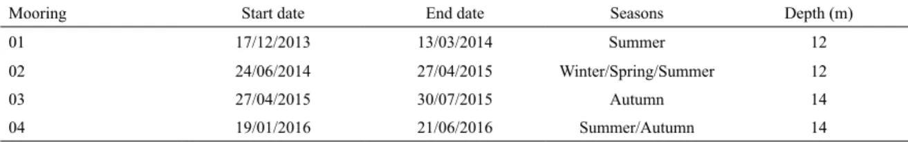
An acoustic wave and current profiler, AWAC/Nortek of 1MHz, recorded four SL data time series that totalized 650 days and had only two interruptions. The first and sec-ond interruptions lasted 100 and 140 days, respectively. The data were measured by a pressure sensor that per-formed a 120-second average every hour. This equipment sampled two points (400m away) during four periods described in detail in Table 1. The AWAC also acquired current velocity and direction profiles, wave parameters, and water temperature; however, this work only aims at studying the SL data. A fifth and last mooring has been recovered after this article has been submitted. The re-covered record forms a series of SL data between May and September 2017. There was no time to perform all the analyzes, however we chose to present an extremely low level event that occurred at the beginning of August in the whole Brazilian coast, which was the subject of several media reports.
An automatic weather station Vaisala MAWS 301, installed and maintained by the National Institute of Meteorology (INMET) from Brazil, provided atmospheric pressure and hourly wind direction and intensity data used in this work. This station is located over 2,000m away from the AWAC mooring in an area free of obstacles with
sensors positioned 10m above SL (Figure 1). Wind data were rotated 20º in relation to True North to be aligned with the orientation of the coast-line and later decomposed into alongshore and cross-shore components, following the methodology described in Miranda (2002).
Since a pressure sensor collected the SL data used in this work, the variation of atmospheric pressure as a func-tion of mean pressure was added. In order to remove the high-frequency oscillations (tidal frequencies), a Lanczos-Cossine low-pass filter (Thompson, 1983) was used, which removes 95% of the oscillations with frequencies higher than 1/40h. The result is the so called low-frequency or subtidal oscillations. The high-frequency oscillations were obtained by the subtraction of subtidal series from the raw, and are referred as tidal frequencies.
The spectral analysis followed the methodology pro-posed by Welch (1967). A type of Hanning window was applied with 50% overlapping, a procedure that results in an estimated mean spectral density calculated from the es-timated five segments. Statistical reliability is improved even though resolution is lost in the process of using spec-tral windowing.
Table 1. Data sampled periods of each mooring.
Mooring Start date End date Seasons Depth (m)
01 17/12/2013 13/03/2014 Summer 12
02 24/06/2014 27/04/2015 Winter/Spring/Summer 12
03 27/04/2015 30/07/2015 Autumn 14
04 19/01/2016 21/06/2016 Summer/Autumn 14
respectively, with values close to -1 and 1 representing the highest correlation. Values near zero do not dem-onstrate an existent relationship. All correlations pre-sented a significance level higher than 99%.
The harmonic analysis performed for the SL data is based on the Fast Fourier Transform, which uses tidal harmonic components for the calculation of amplitudes and phases of tidal harmonic constants, providing the importance of each constituent. The results were ob-tained through the computer program called T-tide, fol-lowing the methodology developed by Pawlowicz et al. (2002).
From the results obtained in the harmonic analysis, the Form number (F) was calculated by dividing the sum of the diurnals O1 and K1 by the semidiurnal constants M2 and S2. Thus, the relative importance of diurnal and semidiurnal constituents is determined and it is possible to classify the tidal regime in a given region by following the classification proposed by Defant (1961), apud Miranda (2002).
The mean tidal range (MTR) resulted from the average of all high SL plus the average of all low SL observed over tidal and subtidal time series. The maximum high and low SL represents the ma-jor and minor amplitudes reached by the water level, respectively.
SL values above and below two standard deviations (STD) were selected for each mooring, and then the maxi-mum and minimaxi-mum SL events were separated from the rest. In order to obtain a seasonal scenario, the number of positive and negative SL events for each season was quantified. Occurrences of values above and below three STDs were also selected, which may be related to extreme events.
RESULTS
The MTR for all tide time series was 0.31m. The av-erage for all subtidal oscillations in the low-frequency time series was 0.37m. The difference between the maxi -mum and mini-mum level in the raw time series was 2.2m.
However, when the high- frequency oscillations (tides) were removed, a maximum variation of 1.62m was found. Nonetheless, when the oscillations caused by tides were analyzed alone, a maximum difference of 0.96m was observed.
On August 12, 2017, the lowest SL was recorded among all the time series, 1.26m below the mean SL (re-corded by mooring 05, not show). This event was greatly accompanied by the media, being called “the super re-treat” of the sea. The SL remained below the mean level for approximately 100 hours, reaching its maximum af-ter 54h of the beginning. This phenomenon was related to a strong meteorological system, an anticyclone on the Atlantic Ocean, that caused intense and persistent south-wards winds on the entire SBCS. It notes that this event occurred at spring tide period.
Table 2 presents in detail the values of tidal and sub-tidal averages for each mooring and the values of the maximum SL at each frequency above and below zero (or mean SL). It is important to notice that SL can reach 1.2m above the mean when adding up tidal and subtidal maxi-mum amplitudes without considering the effect of wave runup.
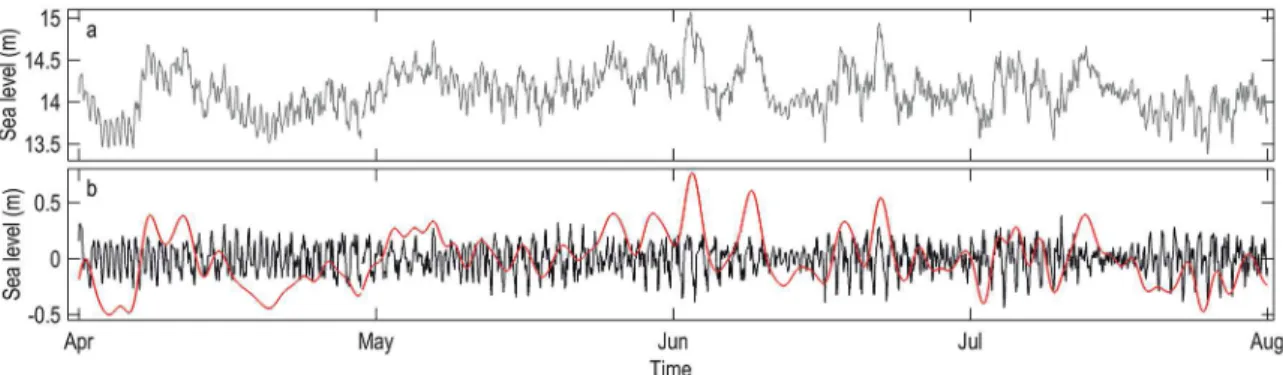
Figures 2a, 3a, 4a and 5a show the raw SL time series for each mooring. Figures 2b, 3b, 4b and 5b (red color) present the SL filtered data, i.e. subtidal oscillations, and in black it is shown the high-frequency or tidal oscilla-tions of SL. It is possible to notice that in most seasons (Figure 2, Figure 3 between September and February, and the beginning of Figure 5) the tidal and subtidal oscilla-tions are proportional in amplitude. However, in Figure 4 and at the end of Figure 5, the magnitude of the amplitude of subtidal oscillations is greater than tidal oscillations. These periods coincide with the winter and autumn sea-sons in the Southern Hemisphere.
Table 2. Mean tidal range (MTR) and SL maximum above and below the zero calculated for tidal and subtidal time series for each mooring.
MTR (m) Maximun above zero (m) Maximun below zero (m)
Tidal Subtidal Tidal Subtidal Tidal Subtidal
Mooring 01 0.33 0.29 0.51 0.40 -0.40 -0.31
Mooring 02 0.31 0.41 0.53 0.64 -0.43 -0.49
Mooring 03 0.30 0.38 0.44 0.66 -0.35 -0.57
Mooring 04 0.30 0.40 0.43 0.55 -0.35 -0.43
Figure 2. SL time series from summer 2014 (mooring 01). a) Raw data. b) Tidal (in black) and subtidal (in red) frequencies.
Figure 3. SL time series from winter and spring 2014 and summer 2015 (mooring 02). a) Raw data. b) Tidal (in black) and subtidal (in red) frequencies.
Figure 5. SL time series from summer and autumn 2016 (mooring 04). a) Raw data. b) Tidal (in black) and subtidal (in red) frequencies.
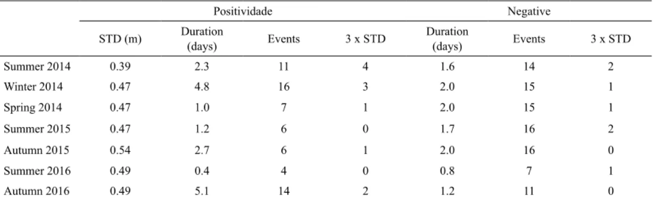
Table 3. Duration and total number of events of SL above (positive) and below (negative) two standard deviations (STD) and three STDs from the raw data series for each season.
Positividade Negative
STD (m) Duration
(days) Events 3 x STD
Duration
(days) Events 3 x STD
Summer 2014 0.39 2.3 11 4 1.6 14 2
Winter 2014 0.47 4.8 16 3 2.0 15 1
Spring 2014 0.47 1.0 7 1 2.0 15 1
Summer 2015 0.47 1.2 6 0 1.7 16 2
Autumn 2015 0.54 2.7 6 1 2.0 16 0
Summer 2016 0.49 0.4 4 0 0.8 7 1
Autumn 2016 0.49 5.1 14 2 1.2 11 0
worth mentioning that these extreme events (three STDs) only occurred during spring tides.
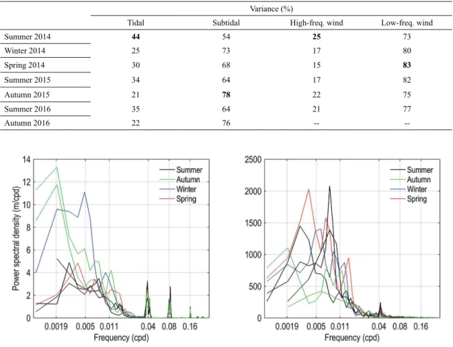
Basic statistical analyses for each season indicated that between 54 and 78% and between 21 and 44% of the SL variance could be attributed to subtidal oscillations and astro-nomical tides, respectively, depending on the season. Table 4 shows in detail the tidal and subtidal variances and the along-shore wind variance at high and low frequencies. The small remaining percentage of approximately 2% is due to other frequencies that are not the object of this study.
The spectral analysis of all SL raw data and the along-shore wind (Figures 6a and 6b) shows a great amount of energy at low frequencies, which corresponds to periods between 20 and 8 days (0.0019 and 0.005cpd). It is also possible to observe that the largest amount of energy in the SL variability occurred in the autumn (green) and winter (blue). These results demonstrate a greater variability of SL and wind speed time series at low frequencies, which also shows a clear relationship between wind and SL vari-ations. It is also possible to observe in Figure 6a a great amount of energy at high frequencies that are associated
with diurnal (25h) and semidiurnal (12h) tides, especially during the summer months (black).
The cross correlation between the alongshore wind and SL for each season resulted in a coefficient between 0.8 and 0.6 with 13 to 17h of time lag. This corroborates with the results found in the spectral analysis, in which the alongshore wind is the main driving mechanism for local SL. The cross correlation between cross-shore wind and SL resulted in a coefficient between 0.6 and 0.3 with 16 to 31h of time lag.
Table 4. Variances of tidal and subtidal oscillations and of the high- and low-frequency alongshore wind for each season.
Variance (%)
Tidal Subtidal High-freq. wind Low-freq. wind
Summer 2014 44 54 25 73
Winter 2014 25 73 17 80
Spring 2014 30 68 15 83
Summer 2015 34 64 17 82
Autumn 2015 21 78 22 75
Summer 2016 35 64 21 77
Autumn 2016 22 76 --
--DISCUSSION
Corroborating with the visual inspection of tidal and subtidal time series (Figures 2, 3, 4 and 5), statistical analy-ses (Table 4 and Figure 6) indicated that, in some seasons, around almost half of the energy involved in SL oscilla-tions could be attributed to tidal oscillaoscilla-tions. These results demonstrated that, even though the averages of astronomi-cal tide amplitudes are considered small by the literature and also by the findings of this paper (0.31m), they are very similar to the calculated average values of subtidal ampli-tudes (0.37m). Thus, not only the variance of tidal oscilla-tions but also the mean amplitude led us to the conclusion that the astronomical tide cannot be totally neglected in oceanographic studies in the RS coast.
Usually in the literature (Rocha et al., 2015; Siegle and Calliari, 2008; Möller et al., 2007), the mean tidal range and the maximum amplitude reached by meteorological tides are compared, causing the misinterpretation that astro-nomical tides do not matter in the local SL oscillations and
consequently in associated processes. This reason led many studies to disregard the astronomical tides in their analyses.
Few research works in the study area have broken this paradigm created by that misinterpretation of data results. Soares et al. (2007) contrasted the cited works by testing the importance of astronomical tides on the SBCS area us-ing numerical simulations. One of the main conclusions was that regional circulation depends on a combination of tides, winds and river plumes.
Spectral analysis of SL and alongshore wind shows that the most part of the energy is found at low frequencies with coincident peaks, demonstrating a clear relationship be-tween wind and SL variations. This can be interpreted as an indication that the wind is an important driving mechanism for local SL oscillations in time scales from hours to days. Another important aspect is the large differences among the SL time series with clear seasonal patterns.
As shown, the wind has a large influence on the lo -cal SL variations, so the wind seasonal variability directly
affects the SL variance. Cold fronts that invert the wind direction reach Southern Brazil more frequently between May and September (austral autumn and winter). From October to April (austral spring and summer), cold fronts are less frequent in this region as they present a more zon-al and maritime displacement (Escobar et zon-al., 2016). This seasonal pattern in SL variability, showing a higher inten-sity of positive extreme events during autumn and winter, has already been observed in a region further north from the study area, also associated with atmospheric frontal systems (Campos et al., 2010).
The results from the cross correlation between the alongshore wind and SL for each season demonstrated the effect of the wind on the SL oscillations. This corroborates with the findings from the spectral analysis, in which the alongshore wind is the main driving mechanism for the local SL. The correlation between wind and water circu-lation had already been demonstrated in previous studies (Costa and Möller, 2011; Andrade et al., 2016), but this is the first time that this was demonstrated with observa -tional SL data in Tramandaí Beach.
The positive coefficients from the correlations can be explained by the Ekman balance model (Ekman, 1905) for the Southern Hemisphere, where southward alongshore winds induce a decrease in the water level (upwelling) and northward alongshore winds cause an increase in it (downwelling). The cross correlation between cross-shore winds and SL resulted in small coefficients, which is an in -dication of their poor relationship. The Ekman transport in the RS coast had already been observed but in association with the water circulation (Andrade et al., 2016; Soares and Möller, 2001).
A larger number of positive maximum events (greater than two STDs) occurred during the winter and autumn, with exception of autumn 2015, when fewer events were observed. However, this can be partially explained by the high STD of this time series (the largest of all). Negative peaks showed a uniform pattern of occurrence between seasons. Extreme atmospheric events such as the passage of intense extra-tropical cyclones happen more frequently in the winter and autumn months (Machado and Calliari, 2016; Saraiva et al., 2003) and thus it can explain the high occurrence of positive peaks in these two seasons.
It is important to note that the peaks reached only by the subtidal frequency are much lower than the peaks as a whole. In other words, a significant SL rise only occurs with the contribution of the astronomical tide. Again, the astronomical tide cannot be totally disregarded in studies
High SL amplitudes may be even greater when con-sidering the wave runup effects in storm events (Scheffner, 2008). Guimarães et al. (2015) used numerical modeling and found amplitudes greater than 2m only caused by the wave runup on Tramandaí Beach, which are above the mean SL. This phenomenon can lead to seawater flooding on coastal areas. Therefore, by adding up the maximum amplitudes of high spring tides (0.53m), the subtidal rise driven by the wind (0.66m), and an extreme wave runup (2m), a dangerously high SL can occur on the beach. In the same article, Guimarães et al. (2015) reported erosional events in the beachfront of the city of Imbé. Although not necessarily caused by maximum tidal and subtidal ampli-tudes, they led to the destruction of natural environments and private properties. When SL rise is associated with strong waves, all the RS coastal zone can be affected by intense coastal erosion and extensive flooding.
Fiore et al. (2009) carried a long-term study on the coastal effects of meteorological tides in Mar del Plata, Argentina. The authors found that the events of meteoro-logical tides suffered an increase in their average number per decade and in their duration, also observing an inten-sification of positive events. The abnormal SL elevation near the coast allows the upper beach to be vulnerable to waves of high amplitudes, consequently causing erosion and damage to the ecosystem and private properties.
On the RS coast, high wave energy and high SL as-sociated with the passage of cold fronts and spring tides can change the characteristics of the superficial beach sediment, but they can also cause beach erosion and dune retreat at rates of the order of dozens of cubic meters and several meters, respectively (Siegle and Calliari, 2008). Since it is located near one of the ciclogenetic regions in South America (Parise et al., 2009), it is regularly subject-ed to the occurrence of storms associatsubject-ed with frontal sys-tems and extra-tropical cyclones. According to da Motta et al. (2015), the RS coastal zone is dominated by waves and the regional processes of erosion and deposition are primarily controlled by the alongshore wave energy flux on the beach. These authors found that the results from 22-year temporal analysis of shoreline movement map-ping showed strong erosional processes mainly in the cen-tral portion of the coast.
is neither spatially nor temporally independent since an ex-treme event in the south would enable the prediction of what will occur further north (Campos et al., 2010).
Finally, in the context of climate change (Mawdsley et al., 2014; PBMC, 2016) and increased occupation of coastal areas (Small and Nicholls, 2003), disregarding the pure drive for scientific knowledge, it is essential to study SL oscillations over the time scales of astronomical tides and those driven by meteorological forcing.
CONCLUSIONS
A mean tidal range equal to 0.31m and a subtidal os-cillation average of 0.37m were found based on a long SL time series with more than 650 days. As those averages are very similar, a new perspective on SL oscillations in Southern Brazil is presented, concluding that it is impor-tant to consider the astronomical tidal oscillations in fu-ture studies on Tramandaí Beach and in surrounding areas. The relative importance of tidal and subtidal movements depends on the season. Generally, it can be stated that sub-tidal oscillations are more intense in the autumn. Spectral analysis and cross correlations between the alongshore wind and SL indicated a clear relationship of meteorologi-cal driving mechanisms and subtidal oscillations. A rela-tively short time lag between wind activity and the subse-quent SL response demonstrates a fast wind action on the water SL dynamics. The passage of intense extra-tropical atmospheric systems with northeastward winds associated with spring tides and waves that have a significant height above average can increase the SL up to 3.2m, causing severe damage to private properties and extensive coastal erosion in the region.
ACKNOWLEDGMENTS
We would like to thank CAPES for funding oceano-graphic campaigns (Edital Ciências do Mar II 43/2013) and for the Doctoral Scholarship destined to the first au-thor. We also thank the Instituto Nacional de Meteorologia (INMET) for providing meteorological data. The authors are grateful to MSc. Orozco for the English review and to the Reviewer for the careful reading of the manuscript and his or her valuable comments and suggestions.
REFERENCES
ANDRADE, M. M., TOLDO Jr, E. E. & NUNES, J. C. 2016.
Variabilidade das correntes na plataforma interna ao largo de
Tramandaí (RS) durante o verão de 2014. Pesquisas em Geo-ciências, 43, 289-298.
CAMPOS, R. M., DE CAMARGO, R. & HARARI, J. 2010. Ca
-racterização de eventos extremos do nível do mar em Santos e sua correspondência com as re-análises do modelo do NCEP
no Sudoeste do Atlântico Sul. Revista Brasileira de Meteoro-logia, 25, 175-184.
CASTRO, B. M. & LEE, T. N. 1995. Wins-forced sea level vari -ability on the southest Brazilian shelf. Journal of Geophysical
Research: Oceans, 100, 16045-16056.
CAVALCANTI, I. F. A. & KOUSKY, V. E. 2009. Frentes frias
sobre o Brasil. In: CAVALCANTI, I. F. A., FERREIRA, N. J.,
JUSTI DA SILVA, M. G. A. & SILVA DIAS, M. A. F. (eds.) Tempo e clima no Brasil. São Paulo: Oficina de Textos. CLARA, M. L., SIMIONATO, C. G., D’ONOFRIO, E. & MO
-REIRA, D. 2015. Future Sea Level Rise and Changes on Tides in the Patagonian Continental Shelf. Journal of Coastal
Research, 31, 519-535.
COSTA, R. & MÖLLER, O. O. 2011. Estudo da estrutura e da
variabilidade das correntes na área da plataforma interna ao largo de Rio Grande (RS, Brasil), no sudoeste do Atlântico Sul, durante a primavera-verão de 2006-2007. Revista da
Gestão Costeira Integrada, 11, 273-281.
DILLENBURG, S. R., TOMAZELLI, L. J. & BARBOZA, E. G.
2004. Barrier evolution and placer formation at Bujuru south-ern Brazil. Marine Geology, 203, 43-56.
DA MOTTA, L. M., TOLDO Jr, E. E., ALMEIDA, L. E. B. & NU
-NES, J. C. 2015. Sandy sediment budget of the midcoast of Rio
Grande do Sul, Brazil. Journal of Marine Research, 73, 49-69.
DOTTORI, M. & CASTRO, B. M. 2009. The response of the Sao
Paulo Continental Shelf, Brazil, to synoptic winds. Ocean
Dynamics, 59, 603-614.
DOTTORI, M., & CASTRO, B. M. 2018. The role of remote
wind forcing in the subinertial current variability in the cen-tral and northern parts of the South Brazil Bight. Ocean
Dy-namics, 68, 677-688.
EKMAN, V. W. 1905. On the influence of earth’s rotation on
ocean currents. Arkiv for Matematik, Astronomi och Fysik, 2, 51-52.
ESCOBAR, G. C. J., SELUCHI, M. E. & ANDRADE, K. 2016. Synoptic classification of cold fronts associated with ex -tremes rainfall over the east of Santa Catarina state. Revista
Brasileira de Meteorologia, 31, 649-661.
FIORE, M. M. E., D’ONOFRIO, E. E. & POUSA, J. L. 2009.
Storm surges and coastal impacts at Mar del Plata, Argentina.
Continental Shelf Research, 29, 1643-1649.
GERMANI, Y. F., FIGUEIREDO, S. A., CALLIARI, L. J. & TA
-GLIANI, C. R. A. 2015. Vulnerabilidade costeira e perda de ambientes devido à elevação do nível do mar no litoral sul
do Rio Grande do Sul. Journal of Integrated Coastal Zone
Management, 15, 121-131.
GUIMARÃES, P. V., FARINA, L., TOLDO Jr, E. E, DIAZ-HERNANDEZ, G. & AKHMATSKAYA, E. 2015. Numeri -cal simulation of extreme wave runup during storm events in
Tramandaí Beach, Rio Grande do Sul, Brazil. Coastal
Engi-neering, 95, 171-180.
JUNG, G. B. & TOLDO Jr, E. E. 2011. Longshore current vertical profile on a dissipative beach. Revista Brasileira de Geofísi-ca, 29, 691-701.
MACHADO, A. A. & CALLIARI, L. J. 2016. Synoptic Systems
Generators of Extreme Wind in Southern Brazil: Atmospheric Conditions and Consequences in the Coastal Zone. Journal of
MARONE, E. & CAMARGO, R. 1994. Marés meteorológicas no
litoral do Estado do Paraná: o evento de 18 de agosto de 1993.
Nerítica (Curitiba), 8, 73-85.
MAWDSLEY, R. J., HAIGH, I. D. & WELLS, N. C. 2014. Glob -al changes in mean tid-al high water, low water and range.
Journal of Coastal Research, 70, 343-348.
MIRANDA, L. B. 2002. Princípios de Oceanografia Física de
Estuários, São Paulo, Edusp.
MÖLLER, O. O., CASTAING, P., FERNANDES, E. H. L. &
LAZURE, P. 2007. Tidal frequency dynamics of a southern Brazil coastal lagoon: choking and short period forced oscil-lations. Estuaries and Coasts, 30, 311-320.
PARISE, C. K., CALLIARI, L. J. & KRUSCHE, N. 2009. Storm
surges and beach erosion in southern Brazil: atmospheric conditions and shore erosion. Brazilian Journal of
Oceano-graphy, 57, 175-188.
PAWLOWICZ, R., BEARDSLEY, B. & LENTZ, S. 2002. Classi -cal tidal harmonic analysis including error estimates in MAT-LAB using T_TIDE. Computers & Geosciences, 28, 929-937.
PBMC (PAINEL BRASILEIRO DE MUDANÇAS CLIMÁTI
-CAS), MARENGO, J. A. & SCARANO, F. R. (eds.). 2016.
Impacto, vulnerabilidade e adaptação das cidades costeiras brasileiras às mudanças climáticas: Relatório Especial do Painel Brasileiro de Mudanças Climáticas. Rio de Janeiro, COPPE - UFRJ.
PUGH, D. T. 1987. Tides, Surges, And Mean Sea-Level, Chip-penham, Antony Rowe Ltd.
ROCHA, R. S., TOLDO Jr, E. E. & WESCHENFELDER, J.
2015. Delimitação do terreno de marinha: estudo de caso no litoral do Rio Grande do Sul. Revista Brasileira de
Cartogra-fia, 67, 1723-1731.
SARAIVA, J. M. B., BEDRAN, C. & CARNEIRO, C. 2003.
Monitoring of storm surges on Cassino Beach, RS, Brazil.
Journal of Coastal Research, 35, 323-331.
SCHEFFNER, N. W. 2008. “Water Levels and Long Waves”.
Coastal Engineering Manual, Chapter 5, Part II. Engineer Manual 1110-2-1100. Washington, U. S. Army Corps of En-gineers.
SIEGLE, E. & CALLIARI, L. J. 2008. High-energy events and short-term changes in superficial beach sediments. Brazilian
Journal of Oceanography, 56, 149-152.
SILVA, A. F., TOLDO Jr, E. E. & WESCHENFELDER, J. 2017. Morfodinâmica da desembocadura da Lagoa de Tramandaí
(RS, Brasil). Pesquisas em Geociências, 44, 155-166.
SMALL, C. & NICHOLLS, R. J. 2003. A Global Analysis of
Human Settlement in Coastal Zones. Journal of Coastal Re-search, 19, 584-599.
SOARES, I. & MÖLLER, O. O. 2001. Low-frequency currents
and water mass spatial distribution on the southern Brazilian shelf. Continental Shelf Research, 21, 1785-1814.
SOARES, I. D., KOURAFALOU, V. & LEE, T. N. 2007. Circula -tion on the western South Atlantic continental shelf: 2. Spring and autumn realistic simulations. Journal of Geophysical
Re-search: Oceans, 112, C04003.
THOMPSON, R. O. R. Y. 1983. Low-Pass Filters to Suppress
Inertial and Tidal Frequencies. Journal of Physical
Oceanog-raphy, 13, 1077-1083.
TOLDO Jr, E. E., ALMEIDA, L. E. S. B., NICOLODI, J. L., AB
-SALONSEN, L. & GRUBER, N. L. S. 2006. O controle da
deriva litorânea no desenvolvimento do campo de dunas e da antepraia no litoral médio do Rio Grande do Sul. Pesquisas
em Geociências, 33, 35-42.
TRUCCOLO, E. C., FRANCO, D. & SCHETTINI, C. A. F. 2006.
The low frequency sea level oscillations in the northern coast of Santa Catarina, Brazil. Journal of Coastal Research, 39, 547-552.
VALENTIM, S. S., BERNARDES, M. E. C., DOTTORI, M. &
CORTEZI, M. 2013. Low-frequency physical variations in the coastal zone of Ubatuba, northern coast of São Paulo State, Bra-zil. Brazilian Journal of Oceanography, 61, 187-193.
VIANNA, H. D. & CALLIARI, L. J. 2015. Variabilidade do sistema
praia-dunas frontais para o litoral norte do Rio Grande do Sul
(Pal-mares do Sul a Torres, Brasil) com o auxílio do Light Detection
and Ranging - Lidar. Pesquisas em Geociências, 42, 141-158.
VILLWOCK, J. A. & TOMAZELLI, L. J. 1995. Geologia
Cos-teira do Rio Grande do Sul. Notas Técnicas. Porto Alegre,
CECO, Instituto de Geociências, UFRGS.
WELCH, P. 1967. The use of fast Fourier transform for the esti-mation of power spectra: A method based on time averaging
over short, modified periodograms. EEE Transactions on
Au-dio and Electroacoustics, 15, 70-73.
WILLIAMS, S. J. 2013. Sea-Level Rise Implications For Coastal Regions. Journal of Coastal Research, 63, 184-196.
WRIGHT, J., COLLING, A. & PARK, D. 1999. Waves, tides, and
shallow-water processes, Houston, Gulf Professional
Pub-lishing.
ZAVIALOV, P., MÖLLER Jr, O. O., CAMPOS, E. 2002. First