VAPOR-LIQUID EQUILIBRIUM CALCULATION FOR SIMULATION OF BIOETHANOL CONCENTRATION FROM SUGARCANE

of Chemical

Engineering

ISSN 0104-6632 Printed in Brazil www.scielo.br/bjce

Vol. 35, No. 02, pp. 341 - 352, April - June, 2018 dx.doi.org/10.1590/0104-6632.20180352s20160278

VAPOR-LIQUID EQUILIBRIUM CALCULATION

FOR SIMULATION OF BIOETHANOL

CONCENTRATION FROM SUGARCANE

Karina Matugi

_{, Osvaldo Chiavone-Filho}

_{, Marcelo Perencin de}

Arruda Ribeiro

_{, Rafael de Pelegrini Soares}

_{and Roberto de Campos}

Giordano

1_{Programa de Pós-Graduação em Engenharia Química, Universidade Federal de São Carlos,} Phone: + (55) (16) 3351-8269, Fax: + (55) (16) 3351-8266, Rodovia Washington Luiz, Km

235, s/n, CEP: 13565-905, São Carlos-SP, Brazil.

2_{Departamento de Engenharia Química, Universidade Federal do Rio Grande do Norte, Phone:} + (55) (84) 3215-3773, Av. Senador Salgado Filho, s/n, CEP: 59066-800, Natal - RN, Brasil. 3_{Departamento de Engenharia Química, Escola de Engenharia, Universidade Federal do Rio} Grande do Sul, Phone: + (55) (51) 3308-3528, Fax: + (55) (51) 3308-3277, Rua Engenheiro

Luis Englert, s/n, Bairro Farroupilha, CEP: 90040-040, Porto Alegre - RS, Brazil.

(Submitted: April 30, 2016; Revised: January 26, 2017; Accepted: January 27, 2017)

Abstract - The robustness of the simulation of bioethanol concentration from sugarcane faces two major challenges: the presence of several minor components and the nonlinear behavior of vapor-liquid equilibrium

(VLE) calculations. This work assesses the effect of simplifications to overcome these difficulties. From a

set of seventeen substances, methanol, n-propanol, isobutanol, 2-methyl-1-butanol and 3-methyl-1-butanol

were selected through the examination of the influence of each minor component on vapor-liquid equilibrium

calculations of ethanol-water-third component systems. The selection procedure was based on Txy diagrams built

using the modified Raoult’s law. The influence of the ratio between the vapor phase fugacity coefficients and of the Poynting correction factor were verified. The accuracy of four correlations for vapor pressure was evaluated, and two functional-group activity coefficient models were scrutinized: the recent Functional-Segment Activity Coefficient (F-SAC) and the UNIFAC-Do model.

Keywords: vapor-liquid equilibrium in ethanol production, vapor pressure, Poynting factor, fugacity coefficient, F-SAC.

INTRODUCTION

In ethanol production from sugarcane, the con-centration process usually comprehends two sets of distillation columns, which are responsible for most of the energy demand. Reboilers consume about 35% of the total heating energy of an autonomous first ge-neration distillery (Dias et al., 2011) to concentrate an

ethanolic mixture from around 0.5% to a requested specification of 92.6-93.8% in mass fraction of etha -nol (Marquini et al., 2007; Dias et al., 2011; Furlan, et al., 2012).The feed stream is sugarcane wine, a multicomponent complex mixture having ethanol and water as major components. Tzeng et al. (2010) repor-ted over 20 contaminants in sugarcane wine during fermentation at laboratorial scale, including alcohols,

esters and organic acids. Batista et al. (2012) reported compositions of the main process streams in industry, identifying 17 minor components, and a fusel oil stre-am with 38.7% of impurities in mass fraction.

The use of a large number of compounds in process simulations brings several difficulties. First, the ther-modynamic models for VLE calculations will have an important increase in the number of required interac-tion parameters, even if group contribuinterac-tion approa-ches are used. Additionally, low concentrations make equilibrium calculations less robust. Finally, the more compounds in the simulation the larger becomes the size of the plant model, once again penalizing the ro-bustness of the numeric methods.

Batista et al. (2012) performed a simulation of a typical ethanol concentration section of an industrial plant for a sugarcane wine containing 17 minor com-ponents. Deviations from industrial data were high for minor components, and parameters of the NRTL model (Non-Random Two-Liquids from Chen et al., 1982) for several pairs of substances had to be estimated with the UNIFAC-Do model (UNIQUAC Functional-group Activity Coefficients - Dortmund), using parameters of functional groups from the Aspen Plus® simulator.

In order to simplify this problem, the sugarcane wine is often assumed to be an ethanol-water binary mixture when the overall process is simulated or opti-mized (Marquini et al., 2007; Dias et al., 2011;Furlan, et al.,2012). For simulation of ethanol dehydration this assumption is also common (Ravagnani et al., 2010; Figueiredo et al., 2011; Benyahia et al., 2014; Dai et al., 2014; Soares et al., 2015).

Considering the system as an ethanol-water bina-ry mixture may not have a substantial impact for the ethanol dehydration process, since its feed stream is hydrous ethanol close to the azeotropic point with less than 0.004 mass fraction of contaminants (Batista et al., 2012). However, in the ethanol concentration step, the composition of minor components through the distillation columns may be significant. Thus, a test to select which substances are essential for a reliable simulation of the process is demanded (Brignole and Pereda, 2013).

Moreover, the vapor-liquid equilibrium in each dis-tillation stage may be sensitive to the presence of minor components, and the successful design and operation of a distillation column for complex systems heavily relies on thermodynamic models (Poling et al., 2000). Valderrama et al. (2012) presented a review about VLE thermodynamic modeling for the alcoholic food industry. The work analyzed binary and ternary sys-tems and concluded that better results were obtained

using Raoult’s modified law rather than equations of state. The NRTL model was more accurate for the sys-tems with available experimental data for estimation of the parameters. The UNIFAC model was indicated for cases without experimental data.

Group-contributions models such as the classical UNIFAC from Fredenslund et al. (1977) or its modified form, the UNIFAC-Do from Weidlich and Gmehling (1987), are indicated for multicomponent mixtures, thus overcoming the requirement of a large set of ex-perimental data for estimation of the model parame-ters. Since the number of functional groups is much smaller than the number of possible molecules, the quantity of required experimental data can be sharply decreased. Recently, Soares and Gerber (2013) created a new group-contribution model, F-SAC (Functional-Segment Activity Coefficient), combining the theore -tical characteristics of the interaction energy between charge segments of COSMO-SAC (Conductor-like Screening Model – Segment Activity Coefficient) from Lin and Sandler (2002) and the empirical appro-ach of the UNIFAC.

The present work shows a simple methodology for selection of components to be taken into account in the feed stream of the ethanol concentration process. Further, a systematic assessment is accomplished, to verify the sensitivity of the VLE calculations with respect to usual simplifying assumptions, vapor pres-sure correlations and thermodynamic models for acti-vity coefficients, highlighting the performance of the F-SAC model.

METHODOLOGY

Vapor-liquid equilibrium calculation

Valderrama et al. (2012) used the gamma-phi ap-proach (Poling et al., 2000) for their equilibrium cal-culations to study alcoholic distillations of musts made from fermented grapes.

i vp i i i iP x P

y =

γ

∫

φ

φ

for the initial stage of selection of minor components,

the term ℑ_i was considered equal to one and equa-tions 1 and 2 reduce to the modified Raoult’s law

vp i i i i P x P

y =

γ

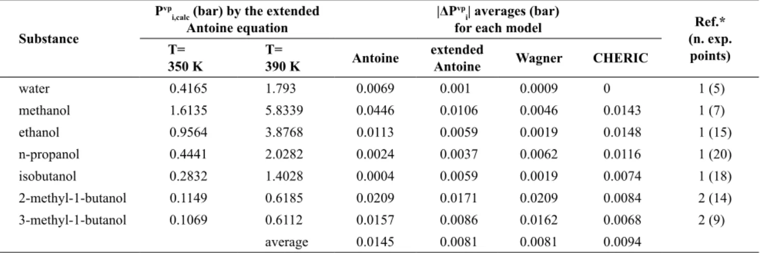
In the present work, four models for vapor pressure were evaluated: the Antoine equation (Antoine, 1888, cited by Thomson, 1946), the extended Antoine equa-tion (from the Design Institute for Physical Properties - DIPPR), the Wagner equation (Wagner, 1973) and the correlation of Chemical Engineering and Materials Research Information Center (CHERIC).

For activity coefficient estimation, the UNIFAC-Do (UNIQUAC Functional-group Activity Coefficients-Dortmund; Weidlich and Gmehling, 1987; Gmehling et al., 1993) model was compared with the recent F-SAC (Functional-Segment Activity Coefficient; Soares and Gerber, 2013; Soares et al., 2013) model.

Functional-Segment Activity Coefficient (F-SAC)

model

The activity coefficient γi for the molecule i in solu-tion may be computed as the sum of a combinatorial or entropic term plus a residual or enthalpic term:

R i C i i

γ

γ

γ

ln = + (5)

The F-SAC model employs the combinatorial term of the UNIFAC-Do model (Weidlich and Gmehling, 1987; and Gmehling et al., 1993). The residual con-tribution comes from the difference between the free energy for charge restoration of a solute molecule i in solution and for charge restoration in a pure liquid i

(Gerber and Soares, 2010):

(

)

ln

γ

where the Gibbs free energy to restore the charge of the solute molecule i in solution is the summation of all n_i.p_i(σ_m) activity coefficients Γ_S with charge seg-ment σ_m

(

)

(

)

∑

i _{n p}

RT G σ σ σ ln * / ₍₅₎

The activity coefficient of each charge segment σ_m is calculated iteratively:

( ) ( ) ( ) ( )             ∆− Γ − = Γ

∑

p m n

n s n s m s σ σ σ σ σ

σ ln exp ,

ln (6)

where the energetic misfit constant αʹ is 8544.6 kcal.Å4_{/mol and the standard contact radius is assumed}

as 1.07 Å. The term EHB _{accounts for hydrogen bond} effects and can be estimated from experimental data.

The σ-profile for each molecule is a summation of the property of the functional groups and these from several charge segments as follows:

(

)

(

)

(

)

2 , 2

, 2 m n

HB n m n m E

W σ σ α σ +σ + σ σ

     ′ = ∆ (7)

( )

_{( )}

∑

p σ ν σ ₍₈₎

( )

{

(

) (

) (

)

}

= k k

o k k k

k Q Q Q

p σ σ , ; 0, ; σ , (9)

If Q_ko _{= Q} k − Qk

+ − Q k

− _{and σ}

k

− _{= −σ}

k

+_Q

k +_/Q

k

− _{, then}

the σ-profile for each functional group is determined by three parameters Q_k+ _{(absolute area with positive}

charge), Q_k− (absolute area with negative charge) and σ_k+ _{(charge density of positive segment).}

Simulation and assessment

Equilibrium calculations were performed through the algorithm introduced by Luyben (2007) with tem-perature updating by the Newton-Raphson method. The program was written in C++ language and run in Codeblocks, a cross-platform IDE. The parameters of the Antoine equation and CHERIC correlation were provided by Poling et al. (2000) and by the CHERIC website, F-SAC parameters by Soares and Gerber (2013) and Soares et al. (2013) and the other parame-ters were taken from the APV82 PURE28 databank of Aspen Plus®_{. The sources of experimental data were}

reported throughout the work.

The comparative analysis was based on the varia-tion between the calculated and experimental values of the property ξ:

exp

ξ

ξ

ξ

∆ calc (10)

Absolute deviation and relative absolute deviations were also used:

exp

ξ

ξ

ξ

∆ calc (11)

.% 100 . exp exp ξ ξ ξ

ξ = −

RESULTS AND DISCUSSION

Minor compounds selection

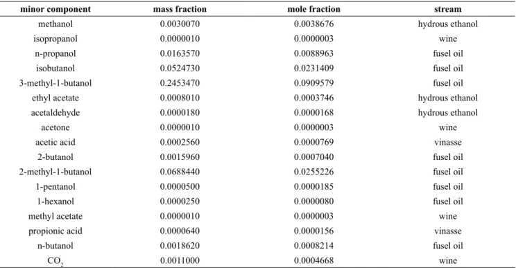
The minor compounds selection procedure started by defining an initial set of substances. The set was chosen based on the data obtained by Batista et al. (2012), since they represent the actual composition of an industrial process. The highest concentration of ea-ch compound, among all the streams of the distillation process, was considered (Table 1).

Next, Txy diagrams were calculated by Raoult’s modified law for each ethanol-water-third component (fixed at its highest mole fraction value indicated in Table1) system, and compared with the calculated cur-ve and experimental data of the ethanol-water binary system. The simulations and the experimental data are at 1.013 bar.

The third components that displayed a significant detachment between the binary and ternary syste-ms were selected. As shown in Figure 1, n-propanol, isobutanol, 3-methyl-1-butanol and 2-methyl-1-buta-nol complied with this condition. Metha2-methyl-1-buta-nol does not follow the condition, but it was also chosen because it is more volatile than ethanol and it is the main contami-nant in the hydrous ethanol stream. Although Hayden O’Connell’s model for organic acids and Henry’s law for uncondensed gases would be more appropriate to the vapor-liquid equilibrium calculations for acetic

Table 1: Highest concentrations (in mass and mole fractions) of each minor component and their stream, from experimental data obtained by Batista et al. (2012).

minor component mass fraction mole fraction stream

methanol 0.0030070 0.0038676 hydrous ethanol

isopropanol 0.0000010 0.0000003 wine

n-propanol 0.0163570 0.0088963 fusel oil

isobutanol 0.0524730 0.0231409 fusel oil

3-methyl-1-butanol 0.2453470 0.0909579 fusel oil

ethyl acetate 0.0008010 0.0003746 hydrous ethanol

acetaldehyde 0.0000180 0.0000168 hydrous ethanol

acetone 0.0000010 0.0000003 wine

acetic acid 0.0002560 0.0000769 vinasse

2-butanol 0.0015960 0.0007040 fusel oil

2-methyl-1-butanol 0.0688440 0.0255226 fusel oil

1-pentanol 0.0000500 0.0000185 fusel oil

1-hexanol 0.0000250 0.0000080 fusel oil

methyl acetate 0.0000010 0.0000003 wine

propionic acid 0.0000640 0.0000156 vinasse

n-butanol 0.0018620 0.0008214 fusel oil

CO₂ 0.0011000 0.0004668 wine

and propionic acids and gas carbonic systems, these substances did not have a noticeable influence.

Assesment of VLE calculation

The pressure in the real process is not atmospheric. Through the columns, the pressure drops from bottom to top. According to Batista et al. (2012), the pressure ranges from 0.9 to 1.6 bar. Temperature varies from 350 to 390 K. These ranges were used to analyze each term of equations 1 and 2, to validate simplifications of the modified Raoult’s law, and to compare models.

Vapor pressure

Figure 1:T-x-y diagrams for ethanol-water-selected minor component at 1.013 bar: experimental data of ethanol-water binary

system at 1.013 bar from Kurihara et al. (1993) (○), calculated curves without (―) and with presence of minor component (―).

Table 2: Vapor pressures (bar) calculated by the extended Antoine equation and averages of absolute deviations (bar) between experimental data and calculated values for the four considered correlations.

Substance

Pvp

i,calc (bar) by the extended

Antoine equation

|ΔPvp

i| averages (bar)

for each model Ref.*

(n. exp. points)

T= 350 K

T=

390 K Antoine

extended

Antoine Wagner CHERIC

water 0.4165 1.793 0.0069 0.001 0.0009 0 1 (5)

methanol 1.6135 5.8339 0.0446 0.0106 0.0046 0.0143 1 (7)

ethanol 0.9564 3.8768 0.0113 0.0059 0.0019 0.0148 1 (15)

n-propanol 0.4441 2.0282 0.0024 0.0037 0.0062 0.0116 1 (20)

isobutanol 0.2832 1.4028 0.0004 0.0059 0.0019 0.0074 1 (18)

2-methyl-1-butanol 0.1149 0.6185 0.0209 0.0171 0.0209 0.0084 2 (14)

3-methyl-1-butanol 0.1069 0.6112 0.0157 0.0086 0.0162 0.0068 2 (9)

average 0.0145 0.0081 0.0081 0.0094

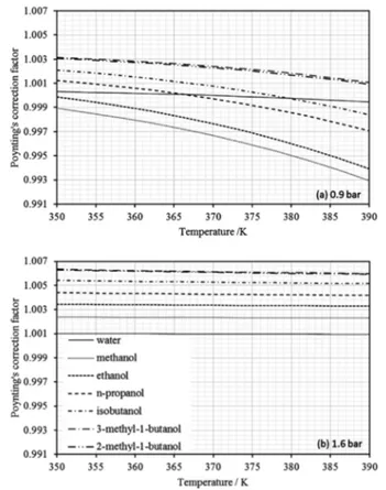
Poynting correction factor

Figure 2 shows a similar behavior of the Poynting correction factor for both minimum and maximum pressures and for all substances. The highest devia-tions from unity were -0.0007 for methanol at 390 K and 0.9 bar, and around 0.006 for 2-methyl-1-butanol and 3-methyl-1-butanol at 350 K at 1.6 bar. In the dis-tillation column, pressure and temperature increase from bottom to top. That means a better representation of the concentration process by the left side of Figure 2.a and the right side of Figure 2.b, in other words, where Poynting correction factors are close to one.

Figure 2: Poynting correction factor with molar volume by DIPPR’s equation and vapor pressure by the extended Antoine equation for the considered temperature range and minimum (a) and maximum (b) pressures.

Ratio between fugacity coefficients

The fugacity coefficients of the saturated pure substances were calculated using the Soave-Redlich-Kwong cubic equation of state in the considered ran-ge of temperature. They deviated from unity when the temperature increased (Figure 3). The farthest values were for methanol and ethanol components, but they are more concentrated in superior stages of the colu-mns, where temperatures are lower.

Figure 3: Fugacity coefficients of the saturated pure substance calculated using the Soave-Redlich-Kwong equation of state with vapor pressures calculated by the extended Antoine equation.

In Figure 4, three substances (water and two whose fugacity coefficient of the saturated pure substance are farther from one) were chosen to illustrate the beha-vior of the ratio between the fugacity coefficients of the pure substance and of the component in the mixtu-re (first term of Equation 2). This ratio ranges between 0.965 at 373 K for water in the water-methanol sys-tem (Figure 4.c) and its highest value is equal to 1.01 at 352 K for ethanol in the methanol-ethanol system (Figure 4.b).

Figure 4.a and the left sides of Figure 4.b and 4.c (with lower temperatures) represent the ethanol con-centration process because methanol has a similar profile as ethanol within the columns. Therefore, the ratio between the fugacity coefficients within the real process will be closer to unity than the value shown in Figure 4.

Activity coefficient

In the last two sections, the two terms of Equation 2 were separately analyzed. The general result of the

multiplication of them (ℑ_i) is a deviation in the se-cond decimal place (above unity for less volatile components and below unity for more volatile ponents). The highest deviations occur when the com-pound is more dilute, in other words, when the activity coefficient of the component reaches its maximum. In consequence, at dilute concentrations, the term ℑi has

* The vapor pressures were calculated by the extended Antoine equation. Experimental data from Gmehling et al. (1982)

Figure 4: Fugacity coefficient of saturated pure substance ϕi

sat, fugacity coefficient of the component in the mixture in the vapor phase V

i

φ

Nine binary systems were selected (Table 3) to test this statement. Calculations of the bubble pressure we-re carried by the modified Raoult’s law using two mo -dels of activity coefficient based on group contribution methods. The results were compared to experimental data with variable temperature and pressure, who-se thermodynamic consistency was reported by the reference. Table 3 also presents deviations obtained by other authors using other two models for activity coefficient (UNIFAC – UNIQUAC Functional-group Activity Coefficients; and NRTL – Non Random Two Liquids).

These results were similar to those obtained by Valderrama et al. (2012) for ethanol-water-third com-ponent ternary systems using three models based on local composition. Higher deviations were observed for more complex molecules.

Although the studied systems of other references might be different from the ones in this work, ac -cording to Table 3, the F-SAC model revealed to be

promising, with a better representation of polar subs-tance interactions.

The limitation of group contribution methods is the inability of discerning isomers such as 2-methyl-1--butanol and 3-methyl-12-methyl-1--butanol. On the other hand, bad fits were attained for simple systems like ethanol--methanol calculated by UNIFAC-Do and water-iso-butanol by both models.

Figure 5 illustrates the calculations for the bi-nary system of greatest interest (ethanol-water) at two temperatures. The two models estimate well the equilibrium.

Table 3: Averages of the relative absolute deviations of pressure and mole fraction of component 1 in the vapor phase *.

System

component 1 – component 2 γi model

Averages of

|∆P|_rel %

Averages of

|∆y₁|_rel % n. pts Ref.*

ethanol – water UNIFAC-Do 1,63 2,43 1476 (1)

F-SAC 1,65 2,28 (1)

ethanol – methanol UNIFAC-Do 16,15 5,48 110 (1)

F-SAC 0,82 0,35 (1)

UNIFAC-Do n.a. 6.1 n.a. (2)

NRTL n.a. 3.5 n.a. (3)

UNIFAC n.a. 6.8 n.a. (3)

ethanol – n-propanol UNIFAC-Do 1,60 0,76 80 (1)

F-SAC 1,46 0,71 (1)

NRTL n.a. 7.5 n.a. (3)

UNIFAC n.a. 7.6 n.a. (3)

ethanol – isobutanol UNIFAC-Do 3,35 0,42 81 (1)

F-SAC 3,53 0,45 (1)

NRTL n.a. 1.4 n.a. (3)

UNIFAC n.a. 1.8 n.a. (3)

ethanol – 2-methyl-1-butanol UNIFAC-Do 0,94 7,80 22 (1)

F-SAC 1,49 8,75 (1)

ethanol – 3-methyl-1-butanol UNIFAC-Do 3,64 0,59 61 (1)

F-SAC 3,10 0,48 (1)

NRTL n.a. 2.3 (3)

UNIFAC n.a. 2.2 (3)

water – methanol UNIFAC-Do 2,21 1,12 898 (1)

F-SAC 2,42 1,13 (1)

NRTL n.a. 2.4 (3)

UNIFAC n.a. 3.7 (3)

water – n-propanol UNIFAC-Do 1,97 1,42 602 (1)

F-SAC 1,79 1,35 (1)

NRTL n.a. 5.9 (3)

UNIFAC n.a. 8.6 (3)

water – isobutanol UNIFAC-Do 18,20 12,94 97 (1)

F-SAC 11,53 9,63 (1)

NRTL n.a. 6 (3)

UNIFAC n.a. 5.8 (3)

water – 3-methyl-1-butanol UNIFAC-Do 8,12 4,00 63 (1)

F-SAC 9,04 4,10 (1)

NRTL n.a. 2.8 (3)

UNIFAC n.a. 35.4 (3)

* For this work: vapor pressure calculated by the extended Antoine equation. Experimental data from Gmehling et al. (1982), except for the ethanol – 2-methyl-1-butanol, from Resa et al. (2005).

Figure 5: Vapor-liquid equilibrium of the isothermal ethanol-water binary system at two temperatures: experimental data from Gmehling et al. (1982) (○)

and calculated curves by UNIFAC-Do model (―) and F-SAC model (- - - ) with vapor pressure calculated by extended Antoine equation.

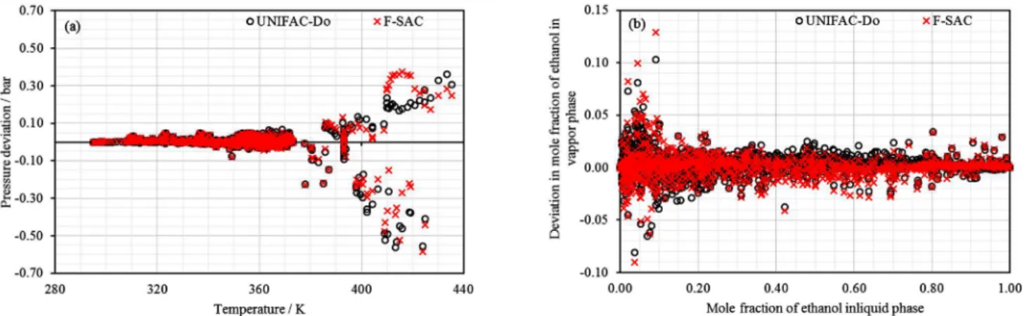
*Vapor pressure calculated by the extended Antoine equation. Experimental data references indicated in table 2.

Figure 6: Deviations in: (a) pressure (bar) as a function of temperature (K), and (b) mole fraction of ethanol in the vapor phase as a function of the mole fraction of ethanol in the liquid phase for the ethanol-water system*.

CONCLUSION

In this paper, five substances (methanol, n-propa -nol, isobuta-nol, 2-methyl-1-butanol and 3-methyl-1--butanol) were selected as most important to be con-sidered in VLE calculations, from a set of seventeen minor components present in the ethanol from the su-garcane concentration process. The used criterion was the influence of each component in the vapor-liquid equilibrium of ethanol-water-third compound system, when compared to the ethanol-water binary system.

the UNIFAC-Do, thus encouraging the use and further development of the first one.

ACKNOWLEDMENTS

The authors would like to thank CAPES (Coordenação de Aperfeiçoamento de Pessoal de Nível Superior), CNPq (Conselho Nacional de Tecnologia e Desenvolvimento Científico) and PRH-ANP (Programa de Recursos Humanos - Agência Nacional do Petróleo, Gás Natural e Biocombustíveis) for financial support.

NOMENCLATURE

Symbols

P_ivp _{vapor pressure of substance i bar}

P Pressure bar

R gases constant m-3_{. bar.K}-1_.mol-1

T Temperature K

V_iL molar volume of liquid

substance i mol.m

-3

x_i mole fraction of component i in the liquid phase

y_i mole fraction of component i in the vapor phase

Greek symbols

∆ Variation bar

γi

activity coefficient of

component i dimensionless

ξ Property

---ϕi

sat fugacity coefficient of saturated

substance i dimensionless

V i

φ

component i in the vapor phase dimensionless

REFERENCES

Agência Nacional do Petróleo, Gás natural e Biocombustíveis (ANP), Consumo de combustíveis no Brasil cresceu 5,28% na comparação entre 2013 e 2014. Electronic document. Rio de Janeiro (2015).

Álvarez, V.H.; Rivera, E.C.; Costa, A.C.; Maciel Filho, R.; Maciel, M.R.W.; Aznar, M. Bioethanol production optimization: a thermodynamic analysis. Applied Biochemistry and Biotechnology, 148, 141-149, (2008).

Aspen Technology, Inc. Aspen Physical Property System. Burlington: Aspen Technology, Inc, (2012).

Batista, F.R.M.; Follegatti-Romero, L.A.; Bessa, L.C.B.A.; Meirelles, A.J.A. Computational simulation applied to the investigation of industrial plants for bioethanol distillation. Computers and Chemical Engineering, 46, 1-16, (2012).

Benyahia, K.; Benyounes, H.; Shen, W. Energy evaluation of ethanol dehydration with glycol mixture as entrainer. Chemical Engineering Technology, 37, No.6, 987–994 (2014).

Brignole, E. and Pereda, S. Phase Equilibrium Engineering. Elsevier, Bahía Blanca (2013).

Čenský, M.; Vrbka, P.; Růžička, K.; Fulem, M. Vapor pressure of selected aliphatic alcohols by ebulliometry. Part 2. Fluid Phase Equilibria. 298, 199–205 (2010).

Chemical Engineering and Materials Research Information Center (CHERIC). Korean Thermophysical Properties Data Bank. Avaiable at: <http://www.cheric.org/research/kdb/hcprop/ cmpsrch.php>. Access in: July 2014.

Chen, C.C.; Britt, H.I.; Boston, J.F.; Evans, L.B. Local composition model for excess Gibbs energy of electrolyte systems.1. single solvent, single completely dissociated electrolyte systems. American Institute of Chemical Engineers Journal, 28, No.4, 588-596 (1982).

Dai, C.; Lei, Z.; Xi, X.; Zhu, J.; Chen, B. Extractive Distillation with a Mixture of Organic Solvent and Ionic Liquid as Entrainer. Industrial & Engineering Chemistry Research, 53, 15786−15791 (2014). Design Institute for Physical Properties (DIPPR).

Sample Chemical Database. Avaiable at: < http:// dippr.byu.edu/students/chemsearch.asp>. Access in: July 2014.

Dias, M.O.S.; Modesto, M.; Ensinas, A.V.; Nebra, S.A.; Maciel Filho, R.; Rossell, C.E.V. Improving bioethanol production from sugarcane: evaluation of distillation, thermal integration and cogeneration systems. Energy, 36, 3691-3703 (2011).

Faúndez, C.A.; Valderrama, J.O. Phase equilibrium modeling in binary mixtures found in wine and must distillation. Journal of Food Engineering, 65, 577–583, (2004).

Fredenslund, A.; Gmehling, J.; Rasmussen, P. Vapor-liquid equilibria using UNIFAC. Elsevier, Amsterdam (1977).

Furlan, F.F.; Costa, C.B.B.; Fonseca, G.C.; Soares, R.P.; Secchi, A.R.; Cruz, A.J.G.; Giordano, R.C. Assessing the production of first and second generation bioethanol from sugarcane through the integration of global optimization and process detailed modeling. Computers & Chemical Engineering, 43, 1-9 (2012).

Gerber, R.P.; Soaes, R.P. Prediction of infinite-dilution activity coefficients using UNIFAC and COSMO-SAC variants. Industrial & Engineering Chemistry Research, 49, 7488-7496 (2010).

Gmehling, J.; Li, J.; Schiller, M. A modified UNIFAC model. 2. Present parameter matrix and results for different thermodynamics properties. Ind. Eng. Chem. Res., 32, 178-193 (1993).

Gmehling, J.; Onken, U.; Grenzheuser, P. Vapor Liquid Equilibrium Data Collection. DECHEMA Chemistry Data Series, Frankfurt (1982).

Kurihara, K.; Nakamichi, M.; Kojima, K. Isobaric vapor-liquid equilibria for methanol + ethanol + water and the three constituent binary systems. Journal of Chemical & Engineering Data, 38, No. 3, 446–449 (1993).

Lin, S.-T.; Sandler, S.I. A priori phase equilibrium prediction from a segment contribution solvation model. Industrial & Engineering Chemistry Research, 41 899-913 (2002).

Luyben, W.L. Process, modeling, simulation, and control for chemical engineers. 2nd edition. McGraw-Hill, Singapore (2007).

Marquini, M.F.; Mariani, D.C.; Meirelles, A.J.A.; Santos, O.A.A.; Jorge, L.M.M. Simulação e análise de um sistema industrial de colunas de destilação de etanol. Acta Scientiarum Technology, 29, No.1, 23-28 (2007).

Perry, R.H. (Ed.); Green, D.W. (Ed.).Perry's chemical engineers' handbook, 8th edition. McGraw-Hill, New York (2008).

Poling, B.E.; Prausnitz, J.M.; O’Connell, J.P., The properties of gases and liquids. 5th edition. McGraw-Hill, New York (2000).

Ravagnani, M.A.S.S.; Reis, M.H.M.; Maciel Filho, R.; Wolf-Maciel, M.R. Anhydrous ethanol production

by extractive distillation: A solvent case study. Process Safety and Environmental Protection, 88, 67-73, (2010).

Resa, J.M.; González, C.; Goenaga, J.M. Density, refractive index, speed of sound at 298.15 K, and vapor-liquid equilibria at 101.3 kPa for binary mixtures of methanol + 2-methyl-1-butanol and ethanol + 2-methyl-1-butanol. Journal of Chemical & Engineering Data, 50, 1570-1575 (2005).

Soares, R.B.; Pessoa, F.L.P.; Mendes, M.F. Dehydration of ethanol with different salts in a packed distillation column. Process Safety and Environmental Protection, 93, 147–153 (2015). Soares, R.P.; Gerber, R.P. Functional-segment activity

coefficient model. 1. Model formulation. Industrial & Engineering Chemistry Research, 52, 11159-11171 (2013).

Soares, R.P.; Gerber, R.P.; Possani, L.F.K.; Staudt, P.B. Functional-segment activity coefficient model. 2. Associating mixtures. Industrial & Engineering Chemistry Research, 52, 11172-11181 (2013). Soave, G. Equilibrium constants from a modified

Redlich-Kwong equation of state. Chemical Engineering Science, 27, 1197-1203 (1972).

Thomson, G.W.M. The Antoine equation for vapor-pressure data. Chemical Reviews, 38, No. 1, 1-39 (1946).

Tzeng, D.-I.; Chia, Y.-C.; Tai, C.-Y.; Ou, A.S.-M. Investigation of chemical quality of sugarcane (Saccharium offcinarum L.) wine during fermentation by Saccharomyces cerevisiae. Journal of Food Quality, v.33, n.2, 2010.

Valderrama, J.O.; Faúndez, C.A.; Toselli, L.A. Advances on modeling and simulation of alcoholic distillation. Part 1: Thermodynamic modeling. Food and Bioproducts Processing 90, 819-831 (2012).

Wagner, W. New vapour pressure measurements for argon and nitrogen and a new method for establishing rational vapour pressure equations. Cryogenics, 13, No. 8, 470-482 (1973).

Weidlich, U.; Gmehling, J. A modified UNIFAC model. 1. Prediction of VLE, hE, and γ∞_{. Industrial}