Inclusive Growth Episodes
March 2019
Abstract
Widening income disparities and slow productivity growth in most advanced, and several emerging-market, economies have rekindled interest in the empirical analysis of the determinants of inclusive growth, defined in this paper as episodes of increases in GDP per capita without a concomitant deterioration in the distribution of household disposable income. The empirical analysis is based on a chronology of inclusive growth episodes between 1980 and 2013 for a sample of 78 countries. Logit and multinomial probit estimations show that human capital accumulation, the redistributive potential of tax-benefit systems, increases in multifactor productivity and labor force participation, as well as trade openness and a range of institutional factors, including political system durability and electoral regimes, are important determinants of the probability of occurrence of inclusive growth. This empirical evidence contributes to the policy debate about how countries can deal with efficiency-equity trade-offs.
JEL: O47, O15, D31
1. Introduction
A combination of slow productivity growth and rising income inequality in most advanced, and several emerging-market, economies has rekindled interest in the empirical links between economic growth and income distribution. In particular, although the specific channels through which growth and income distribution are related are complex and often difficult to disentangle empirically, there is increasing, albeit weak, cross-country evidence that income inequality undermines growth1 and policy initiatives which are growth-friendly often do affect social groups differently.2
Of particular interest in this strand of literature is the experience of countries that have managed to sustain spells of uninterrupted output growth without a concomitant deterioration in the interpersonal distribution of income. In fact, these episodes, which we characterize as inclusive growth, are not infrequent. Nor are they circumscribed to specific regions or time periods. For example, on the basis of the data available from the World Bank’s World Development Indicators (WDI), there are 268 episodes of increases in GDP per capita without an associated deterioration in the distribution of household disposable income in the sample of countries for which information is available for the period 1980-2013.3
Based on this chronology, we estimated pooled logit and multinomial probit models to gauge empirically the determinants of inclusive growth episodes. We started by looking at a variety of output growth and income distribution covariates, including indicators of the population’s educational attainment, the size and redistributive potential of tax-benefit systems, as well as indicators of demand and economic structure, including trade openness, inflation and unemployment. We also looked at various measures of financial deepening, infrastructure and institutional characteristics that are known to influence growth and income distribution. We tested for the robustness of our empirical findings by looking at alternative estimators and different sets of growth and income distribution covariates.
1 See, for example, Washington Centre for Equitable Growth (2015) and OECD (2015a) for reviews of the empirical literature.
2 See, for example, Causa et al. (2014) and OECD (2015b).
3 These episodes include, for instance, France between 1985 and 1989, Germany between 1995 and 1997, Brazil between 2004 and 2006, and India between 1998 and 2000.
We depart from the literature by focusing on a chronology of episodes linking growth to income distribution, rather than estimating (jointly or independently) growth and income distribution equations and testing for specific channels of causality. In this regard, our approach is akin to that of Anand et al. (2013), who also identify episodes of inclusive growth on the basis of changes in GDP per capita and the distribution of income for a selected group of countries. We nevertheless use different estimation techniques and look at additional macroeconomic and institutional variables that can shed light on the likelihood of an inclusive growth episode.
Our main findings are that the probability of an inclusive growth episode rises with increases in human capital accumulation, redistribution through the tax-benefit system, labor force participation and multifactor productivity, as well as trade openness, and it falls with a rise in inflation, output volatility and unemployment. Also, we show that institutions matter, and inclusive growth episodes are more likely in countries with durable political systems, regular parliamentary elections and electoral regimes based on proportional representation. Moreover, although the empirical findings are somewhat weaker, financial deepening, as reflected in an increase in different measures of the stock of credit in the economy, reduces the probability of an inclusive growth episode, probably because of its association with a higher probability of occurrence of banking and financial crises, which are in turn detrimental to growth and improvements in the distribution of income.
The remainder of the paper is organized as follows. Section 2 reviews the literature. Section 3 outlines the empirical methodology and Section 4 describes the data. Section 5 presents and discusses the main results. The last section concludes.
2. Insights from the Literature
Economic theory predicts a trade-off between equity and efficiency: for countries that are already on, or close to, the technological frontier, the distribution of income can only be improved by sacrificing growth (Acemoglu et al, 2012; Andersen and Maibom, 2016). To test this prediction, the empirical literature has looked at the determinants of growth and income distribution separately, often by including synthetic metrics of income distribution, such as the Gini coefficient and quintile income shares, in augmented Solow-type equations using pooled or cross-sectional data. Empirical evidence is
nevertheless mixed, with a few studies suggesting a negative relationship between income distribution and growth (e.g., Clarke, 1995; Deininger and Squire, 1998; Berg and Ostry, 2011; Ostry et al. (2014); Brueckner and Lederman, 2015).4
As for causality running from growth to income distribution, the empirical literature also reports mixed results. For example, Alesina and Rodrik (1994) and Alesina and Perotti (1996) find a negative relationship, whereas Li and Zhou (1998) and Forbes (2000) find a positive relationship, with Deininger and Squire (1996), Ravallion and Chen (1997), Easterly (1999), Barro (2000), Dollar and Kraay (2002), and Lopez (2004), among others, reporting no correlation at all between these variables. In any case, the linkages between growth and income distribution depend on initial conditions, such as the level of income, the incidence of poverty and the extent of asset inequality in a country. They are also affected by a host of slow-moving, structural parameters, such as geography, demography, governance and politics (World Bank, 2005).
The literature has also looked at the relationship between growth and inequality simultaneously. Rather than including income distribution indicators directly in augmented Solow-type equations, as in the traditional growth literature, Hermansen et al. (2016) and Causa et al. (2016) focus on the joint estimation of the distributional effects of a variety of stylized structural (supply-side) reforms in OECD countries. They find that the benefits of growth do trickle down, albeit differently, to different social groups. The papers combine macro-level estimates of the impact of structural reforms on growth with micro-level estimates of the impact of structural reforms on household incomes across the income distribution. The authors find that structural reforms, in particular those related to social protection, affect inequality especially among the lowest income deciles. More recent strands of the empirical literature have benefited from the availability of more granular inequality data including at the sub-national level.5
4 Investment and the distribution of assets, including land, are important channels through which inequality affects growth. These findings are consistent with the theoretical model developed by Galor and Zeira (1993), which relates income inequality to economic growth via credit market imperfections and indivisibilities in investment.
5 For example, Bartolini and de Mello (2016) look at the effects of intergovernmental fiscal relations on growth and income distribution within, not only between, countries. Such approach, however, goes beyond the scope of this paper.
Where positive effects have been found, the literature has focused on identifying the specific policy levers that can be considered ‘super pro-poor’ in that they can generate inclusive growth by delivering stronger growth together with improvements in the distribution of income. Indeed, Lopez (2004) surveys the literature and finds that macroeconomic stability, measured by inflation, as well as policies that aim to enhance educational attainment and infrastructure tend to deliver ‘win-win’ outcomes by enhancing growth and equalizing the income distribution. These findings are consistent with most of the empirical evidence reported below.
The strand of literature that is closest to our analysis focuses instead on specific definitions of inclusive growth based on the concept of generalized concentration curves following Ali and Son (2007). The idea is that social welfare increases with growth but falls with income transfers from poor to rich individuals. As a result, a combination of changes in GDP per capita, to capture the growth dimension, and in the distribution of income can be used to define episodes of inclusive growth using cross-country aggregate data. In this context, growth is defined as inclusive if it increases social welfare, which depends on the opportunities available to the population, and how those opportunities are shared among the population. Evidence is provided for education and health care in the Philippines using data for 1998 and 2004.
Other studies have indeed been based on this idea. For example, Anand et al. (2013) provide evidence based on panel data for a broad sample of countries during 1970-2010 and highlight the importance of education, investment and trade openness as determinants of inclusive growth. While we also find evidence of the importance of these drivers, we use different estimation techniques and look at additional macroeconomic and institutional variables that can shed light on the likelihood of occurrence of inclusive growth episodes. Atkinson and Brandolini (2010) and Dollar et al. (2015) also rely on the social welfare approach to relate changes in inequality and growth using large sets of cross-country aggregate data.
3. Empirical Approach 3.1. The testable hypotheses
This section identifies possible channels through which policy and non-policy variables influence changes in growth and the distribution of income. A few key mechanisms can be highlighted.
Economic growth: when is it inclusive?
The hypothesis that economic growth is associated with a better distribution of income needs to be tested empirically. As noted above, while economic growth brings with it greater material prosperity, it is not always true that the benefits of growth are shared equitably in society, resulting in an improvement in the distribution of income. The experience of Latin America indeed shows that economic growth, which many countries in the region managed to sustain during the 1990s and 2000s, is a weak predictor of the dramatic improvement in the distribution of income that the region has experienced since the turn of the millennium. Several Latin American countries, including Brazil, Argentina, Bolivia, Chile, Colombia and Peru are among the inclusive growth episodes identified in our chronology, but the empirical literature shows that the causal links between growth in real GDP per capita and improvements in the distribution of income are tenuous in the region (Brezzi and de Mello, 2016).
Social protection: the role of tax-benefit systems
Tax-benefit systems are the main policy instruments to redistribute income ex post in advanced economies, and their effects on growth depend on disincentives to labor supply and other distortions that have a detrimental impact on efficiency, as discussed above. In developing countries and emerging-market economies, tax-benefit systems are less developed and therefore potentially less redistributive, essentially on account of lower revenue-to-GDP ratios, greater reliance on indirect taxes, lower progressivity in direct tax schedules and less comprehensive formal social safety nets. In the case of Latin America, for example, incidence analysis shows that the redistributive impact of tax-benefit systems varies considerably from country to country, and it tends to be stronger in Argentina,
Brazil and Uruguay (Brezzi and de Mello, 2016), although they are considerably less redistributive than in advanced economies.
Education and skills: the role of productivity and skill premia
The accumulation of human capital and skills is an essential driver of both productivity, and ultimately GDP growth, and income distribution. Indicators of educational attainment and quality of education are standard regressors in any Solow-type growth regression. At the same time, an increase in the supply of better educated workers tends to be associated with lower skill premia, measured as the increase in wages associated with an additional year of schooling or qualification, which is in turn likely to be associated with lower wage dispersion. Again, the experience of Latin America is illustrative: educational attainment improved rapidly in several countries throughout the 1990s, leading to a reduction in returns to schooling and, as a result, labor income inequality, although skill premia remain high in the region.6 At the same time, increased dynamism in sectors, such as services, which require relatively low skilled workers, has created demand for workers with lower skills.
Structural reforms: shifting resources and rewards
Economic growth ultimately depends on the ability of an economy to push the productivity frontier through innovation and technological prowess or move towards the frontier by shifting resources from lower to higher-productivity sectors or activities. Policy action to support innovation, promote competition in product markets, deepen financial markets, for example, are all growth-enhancing but not necessarily equalizing, given the balance of ‘winners’ and ‘losers’ from pro-growth reforms. While there is a considerably large body of empirical analysis on the growth effects of a variety of structural reforms, especially for developed countries, evidence is still limited on their distributional impacts. As far as the advanced economies are concerned, it seems that some pro-growth policies that raise GDP through increased productivity, such as support for innovation, may lead to technology-driven widening of the wage distribution among employed workers (OECD, 2015b). Other policies that promote labor force participation and job creation also widen the wage dispersion, but this
6 According to OECD calculations, workers with tertiary education or equivalent advanced research qualifications earn about 250 percent more than those with secondary education in Brazil (over 300 percent in Chile), against the OECD average of about 175 percent (OECD, 2014), suggesting that skill premia remain comparatively high in Latin America.
effect may be offset at least in part through job creation, not least among lower-skilled workers. By contrast, reforms to improve access to education, active labor market policies and growth-friendly tax and transfer systems tend to be equalizing in the sense that they tend to reduce wage dispersion and/or household income inequality.
Trade and current account liberalization are important drivers of growth by facilitating access by domestic producers to imported inputs embodying more modern technologies, creating competition in domestic product markets and also possibly removing impediments to foreign investment. The distributional effects of liberalization are nevertheless difficult to gauge and depend on the relative demand for skills and the composition of job creation and destruction in different markets. For example, the reduction of import tariffs that took place in many Latin American countries during the 1990s as part of broader economic liberalization programmes affected sectors that were relatively intensive in unskilled labor. The attendant increase in demand for skills could not be met by a concomitant expansion of supply, resulting in a deterioration in the distribution of income (Gasparini and Lustig, 2011). Skill-saving technological progress often follows trade liberalization is likely to have compounded this unequalising effect. While this is indeed the case in most Latin American countries, Brazil seems to have been an exception in that trade liberalization led to a change in relative prices in the first half of the 1990s that benefited unskilled workers, leading to a fall in the skill premium (Ferreira et al., 2007).
Other factors: demand management and the external environment
Other factors, such as broad macroeconomic management and changes in the external environment, also contribute to growth and changes in the distribution of income. High inflation and output volatility have a detrimental effect on potential growth and also penalize the worse-off and vulnerable social groups who are less well equipped than the better-off to insure themselves against the associated job and real income losses.
Terms-of-trade gains are also associated with stronger growth, at least in the short term, but their effect on the distribution of income depends on the relative demand for skills in the tradable and non-tradable sectors. Again, the experience of Latin America is illustrative, given that the inclusive
growth episodes that the region has observed over the last two decades have coincided in many countries with sizeable gains in their terms of trade as a result of the concomitant long commodity price cycle. However, empirical evidence suggests that these gains in the terms of trade have supported growth, but they have not played a dominant role in explaining the reduction in income inequality in the region (Gasparini et al., 2011; de la Torre et al., 2012).
3.2. The estimating equations
We define an inclusive growth episode (IG) for country i at time t as the combination of growth in GDP per capita without a concomitant deterioration in the distribution of household disposable income between t-1 and t. Based on this bivariate characterization, we estimate logistic regressions to assess the likelihood of an inclusive growth episode and test the channels identified above (economic growth, social protection, education and skills, and structural reforms), while controlling for other determinants of growth and income distribution.7 In particular, we estimate the following model:8
Prob(IG 1|X) (i X' ),α
(1) where α is a vector of the parameters to be estimated, X is a vector of exogenous variables, and
Φ(⋅) is the logistic function.9
The structural model associated with model (1) can be written as:
* it * it it IG X , IG 1 if IG 0, and 0 otherwise. i it it α (2)
with i = 1, …, N; t = 1, …, T; i captures the unobserved individual effects; and it is an error
term.
We also estimate an multinomial probit model (MNP) to take account of alternative combinations of growth in GDP per capita and changes in inequality.10 The MNP model is used with
7 This is akin to the methodology proposed by Aoyagi and Ganelli (2015), who consider the direct impact of a fixed block of structural determinants, coupled with a set of controls.
8 For details on this binary choice model see, for example, Greene (2012, Ch. 17).
9 We should note that, as probit models do not render themselves well to the fixed-effects treatment due to the incidental parameter problem (Wooldridge, 2002, Ch. 15, p. 484), we estimate a logit model with fixed-effects.
discrete dependent variables that take on more than two outcomes that do not have a natural ordering. In our context, there are three other possible combinations of growth in GDP per capita and changes in income distribution that can be considered: i) non-positive growth in GDP per capita with deterioration in income distribution; ii) non-positive growth in GDP per capita with no deterioration in income distribution; and iii) positive growth with deterioration in income distribution.
In the MNP model, the choice probabilities among a set of categorically distributed alternatives (in our case, four) are simultaneously estimated.11 The stochastic error terms for the implementation of this model are assumed to have independent, standard normal distributions. Evaluating the likelihood function involves computing probabilities from the multivariate normal distribution.12
These combinations can therefore be used to define an alternative dependent variable: 0
(non-positive growth, deterioration in income distribution), 1 (non-(non-positive growth, no deterioration in income distribution), 2 (positive growth, deterioration in income distribution), and 3 (positive growth, no deterioration in income distribution). Option 3 corresponds to the inclusive growth case discussed
above. In particular, the dependent variable “IG=1” in Model (1) can be replaced by “IG=0,1,2,3” in the multinomial probit estimations in our panel dataset.
3.3. The data
We use annual data on real GDP per capita available from the IMF’s International Financial Statistics (IMF’s IFS) database and on the Gini coefficient of the distribution of income from the Standardized World Income Inequality Database (SWIID). We consider the Gini coefficient for income both gross and net of taxes and government transfers, and from alternative sources, including UN WIDER, the University of Texas Inequality Project (UTIP) and the World Bank.
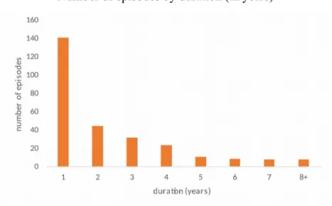
Our data set includes 46 to 78 countries between 1980-2013, depending on the income distribution measure used. The number of inclusive growth episodes in our chronology is 268 with an average duration of 2.5 years. Most episodes last one year (Figure 1), although longer episodes, lasting
11 MNP was the chosen method since the alternative, a multinomial logit model (MNL) assumes the independence of irrelevant alternatives (IIA). A violation of the IIA assumption results in inconsistent estimates. To test for a potential violation of the IIA assumption, we performed a Hausman-McFadden test and a Small-Hsiao test. Because the results of both the Hausman-McFadden and Small-Hsiao tests did not point at a confirmation of the IIA assumption, we could not safely use the MNL estimation and decided in favor of the MNP.
12 See Cameron and Trivedi (2005, chap. 15) for a discussion of multinomial models, including multinomial probit. Long and Freese (2014, chap. 8) discuss the multinomial logistic, multinomial probit and stereotype logistic regression models.
5 years and more, are not infrequent. The average growth rate of real GDP per capita is about 3.3 percent in an episode, and the average reduction in the Gini coefficient is about 0.8. While duration does not seem to have much influence on the magnitude of changes in real GDP per capita, the reduction in the Gini coefficient tends to be more pronounced in episodes that last 4 years or less (Figure 2).
Figure 1. Frequency of inclusive growth episodes, 1980 - 2013
Number of episodes by duration (in years)
Source: Authors’ calculations.
Figure 2. Magnitude of inclusive growth episodes, 1980 - 2013
Average change in real GDP per capita and the Gini coefficient by duration (in years)
Source: Authors’ calculations.
The set of regressors used in the estimations are as follows. To test for the growth channel, we include in the baseline specification the rate of growth of real GDP per capita (from IMF’s IFS), the
rate of growth of labor productivity (computed as output per worker) and the rate of change in labor force participation (LFP) (both from World Bank’s WDI database). The social protection channel is tested by including in the baseline regression the difference between the Gini coefficients on gross and net income to measure the redistributive potential of tax-benefit systems (as in Ostry et al., 2014). The education/skills channel is tested by including in the baseline regression an index of human capital, based on the number of years of schooling (data from Barro and Lee, 2013). Finally, to test for the demand management and external environment channel, we include a number of indicators from IMF’s IFS, such as the degree of trade openness (defined as exports plus imports over GDP), the 5-year rolling standard deviation of real GDP growth to proxy for output volatility (authors’ computation), the rate of CPI inflation (annual change in the log of CPI) and the unemployment rate (in percent).
We control for level of development, which proxies for a country’s distance to the technological frontier, by using the lag of real GDP per capita. We also experiment with alternative controls (retrieved from the IMF’s IFS and World Bank’s WDI databases), such as the share of exports in GDP, changes in the terms-of-trade, the shares of employment in agriculture and industry (in percent), the value added of agriculture in percent of GDP and the duration (in years) of identified inclusive growth episodes to control for possible hysteresis effects.
We look at how the occurrence of inclusive growth episodes depends on infrastructure development by testing for several different indicators, including paved roads per capita, kilometers of roads, kilometers of paved road, number of hospital beds per capita, number of sanitation facilities per capita, rural water source per capita, kilowatts of electricity production, and number of mobile and land line subscriptions per capita. These data are available from the World Bank’s WDI database.
To shed more light on the effects of economic volatility, we experiment with indicators of financial crises, defined as dummy variables taking the value of one when a crisis occurs, and zero otherwise. They include domestic and foreign debt crises, currency crises and banking crises. The classification and identification of crisis episodes is available from Reinhart and Rogoff (2011). We also rely on Leaven and Valencia (2010) to distinguish between systemic and non-systemic financial crises.
As a robustness check, we also experiment with several indicators of government expenditure, including total spending and outlays on agriculture, education, health care, defense, transport and communication, social protection and mining. Data come from the Statistics of Public Expenditure for Economics Development (SPEED) put together by Yu et al. (2015), and all items are defined in real per capita terms.
Data on political and institutional variables are available from the Polity IV project and Database of Political Institutions (DPI) (Beck et al., 2001). These include: the number of years in office of the chief executive, checks and balances, whether a legislative election took place, whether the electoral system is based on proportional representation or majority, the margin of majority (defined as the number of government seats divided by total seats in the legislature), the Polity2 summary indicator of institutional quality (whose core is computed by subtracting the autocracy score from the democracy score, resulting in an unified polity scale ranging from +10 (strongly democratic) to -10 (strongly autocratic)), the durability of the political regime in years, the constraints on the executive and the Polity fragmentation or decentralization.13
Financial development is measured by a set of variables retrieved from the Global Financial Development Database (GFDD) put together by Čihák et al. (2012). The database covers 203 economies and includes measures of size of financial institutions and markets (financial depth), the degree to which individuals can and do use financial services (access), the efficiency of financial intermediaries and markets in intermediating resources and facilitating financial transactions (efficiency), and the stability of financial institutions and markets (stability). We rely on the following variables: bank private credit, deposit money bank assets, liquid liabilities, central bank assets, private credit by deposit money banks and other financial institutions, stock market capitalization, bank deposits and global leasing volume (all in percent of GDP), as well as net interest margins and the spread between lending and deposit rates (both in percent).
13 Note that some of the political variables considered may have non-linear effects. For instance, too many or too few years in which the chief executive is in power may affect inclusive growth differently. We tested this empirically and the higher-order term came out statistically insignificant. We thank the editor for suggesting this additional robustness check.
4. Empirical results 4.1. Logit models
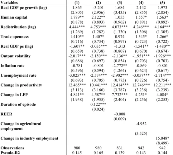
The results of the logit estimation of model (1) are reported in Table 1. While output growth seems to be a poor predictor of inclusive growth episodes, this is not the case of changes in multifactor productivity and labor force participation. The social protection and education/skills channels are also important and fairly robust across specifications: more redistributive tax-benefit systems and better educational outcomes14 are both associated with a higher probability of occurrence of an inclusive growth episode. Demand management and the external environment also matter: the more an economy is open to trade15 the higher is the probability of occurrence of an inclusive growth episode, but the higher the rates of inflation and unemployment, and the volatility of output, the lower is the probability of occurrence of an inclusive growth episode (although not always at conventional levels of statistical significance in the case of inflation). Moreover, less developed countries have a lower probability of occurrence of an inclusive growth episode, despite the hypothesis that distance from the technological frontier is expected to increase the likelihood of an inclusive growth episode.
To shed more light on the role of structural factors, it can be argued that inclusive growth episodes are due to a combination of policies that complement and reinforce each other, creating a virtuous circle that in turn makes inclusive growth episodes more durable. To test this hypothesis, we included among the regressors an indicator of the duration of inclusive growth episodes (in number of successive years a country has sustained non-negative growth in GDP per capita and improvements in the distribution of income). The empirical findings indeed show that duration matters: the longer a country can sustain inclusive growth the higher the probability of occurrence of an episode. In the same vein, we experimented with restricting the sample to exclude short-lived inclusive growth episodes, or those defined as lasting only one year. The estimations, reported in Table A1 in the appendix, show that while coefficients lose some statistical significance, signs and qualitative findings hold. 16
14 Results (available upon request) are also robust to alternative proxies, such as the inclusion of either primary school enrolment per capita or secondary school enrolment per capita.
15 Using instead terms of trade or the share of exports in GDP yields qualitatively similar results (not shown). 16 We thank the editor for making this point.
Moreover, we extended the baseline specification to include the real effective exchange rate, as well as the shares of employment in agriculture and industry. We find that, whereas an appreciation of the real effective exchange rate does not statistically affect the probability of occurrence of an inclusive growth episode, increases in the share of population working in industry (but not in agriculture) rise the likelihood of an inclusive growth episode taking place.17
Table 1: Determinants of inclusive growth: Bivariate specification, baseline model
Variables (1) (2) (3) (4) (5)
Real GDP pc growth (lag) 1.865 -3.201 1.684 2.142 1.973 (2.805) (2.956) (3.435) (2.855) (2.854) Human capital 1.789** 2.122** 1.055 1.557* 1.563* (0.878) (0.893) (0.962) (0.891) (0.892) Redistribution (lag) 4.444*** 4.753*** 4.073*** 4.246*** 4.164*** (1.269) (1.282) (1.330) (1.306) (1.305) Trade openness 1.410** 1.407* 0.974 1.345* 1.266* (0.716) (0.734) (0.897) (0.723) (0.722) Real GDP pc (lag) -1.607** -3.035*** -1.313 -1.541** -1.480** (0.659) (0.738) (0.807) (0.670) (0.674) Output volatility -2.017*** -2.150*** -2.136** -1.951*** -1.926*** (0.686) (0.697) (0.854) (0.703) (0.703) Inflation rate -0.781 -0.801 -2.772** -0.869 -0.801 (0.596) (0.594) (1.264) (0.624) (0.617) Unemployment rate -3.025*** -2.574*** -2.902*** -3.057*** -2.714*** (0.693) (0.705) (0.773) (0.726) (0.754) Change in productivity 12.465*** 10.441*** 12.414*** 12.746*** 12.211*** (3.113) (3.166) (3.787) (3.236) (3.239) Change in LFP 4.841** 4.587** 7.732*** 4.251* 4.084* (1.938) (1.955) (2.404) (2.256) (2.253) Duration of episode 0.122*** (0.024) REER -0.008 (0.009) Change in agricultural employment -4.952 (3.525)
Change in industry employment 15.048*
(8.499)
Observations 980 980 831 942 942
Pseudo-R2 0.145 0.165 0.139 0.143 0.144
Note: All models are estimated by logit. Standard errors are reported in parenthesis. The constant term is not reported for parsimony. *, **, *** denote statistical significance at the 10, 5, and 1 percent levels, respectively. LFP and REER denote, respectively, labor force participation and real effective exchange rate.
Source: Authors’ estimations.
17 The real effective exchange rate has a bearing on growth and the distribution of income by effecting the relative price of tradables and non-tradables. To the extent that productivity is higher in sectors producing tradables, a high real effective exchange rate discourages a shift in resources towards higher-productivity activities, which is growth-enhancing, but it leads to income gains for workers in the non-tradable sector, the overall effect on the income distribution depending on the composition of the work force between these sectors.
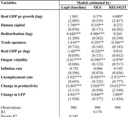
4.2. Robustness to different estimators
To test for the robustness of the results of the logit regressions, we re-estimated the baseline model by OLS and a rare events logit (or relogit) estimator. In a logistic regression, the Maximum Likelihood estimates are consistent but only asymptotically unbiased. The basic problem is having a number of units (inclusive growth episodes) in a panel that has no events. This means that the country-specific indicators corresponding to the all-zero countries perfectly predict the zeroes in the outcome variable (Gates, 2001; King, 2001). This is a well-known phenomenon in the statistical literature (for an overview see Gao and Shen, 2007). The simplest way of dealing with this problem is decreasing the rareness of the event of interest:18 by lowering the threshold of what constitutes the event of interest or expanding the data selection period, for example, there is less need to correct for rareness. Alternatively, the King and Zeng’s (2001) bias correction method, the relogit estimator, can be used.19
The relogit estimator for dichotomous dependent variables provides a lower mean square error in the presence of rare events and can be defined as follows:
it Prob(IG 1|Zit) ( 'Z it)Prob(IGit 1|Sit, X )it (iSit'ηXit' )γ , (5) with i = 1, …, N; t = 1, …, T, where
' ' X ' 1 1 1 eZit 1 eiSit it η γ,
, , are the vectors ofthe parameters to be estimated, and Φ(⋅) is the logistic function.
The parameters can be estimated by maximum likelihood, and the variance of the estimated
coefficients can be expressed as
Var
(
^ϑ
)
=
(
Z 'VZ
)
−1 , where V is a diagonal matrix, with diagonal entries equal to Φ(¿)⋅[1−Φ(¿)] . In the case of rare events, Φ(¿) will be generally small. However, aspointed out by King and Zeng (1999a, 1999b, 2001), the estimates of Φ(¿) and Φ(¿)⋅[1−Φ(¿)]
among observations that include rare events (in our case, for which IG = 1) will be typically larger
18 For this reason, we also include in the baseline regressions (and robustness that follow) episodes of inclusive growth of one year in duration to minimize this rare-events potential problem.
than those among observations that do not include rare events (i.e., for which IG = 0). Consequently, their contribution to the variance will be smaller, rendering additional ‘rare’ events more informative than additional ‘frequent’ events. Therefore, we follow King and Zeng (1999a, 1999b) and correct for the small sample and rare events biases and estimate a relogit model where the sampling design is random or conditional on Zit.20
The regression results are reported in Table 2. While the parameter estimates obtained by OLS are similar to the baseline ones estimated by logit, lagged growth becomes statistically significant in the relogit regression, whereas the education/skills and social protection channels lose significance.
Table 2: Determinants of inclusive growth: Bivariate specification, alternative estimators
Variables Models estimated by:
Logit (baseline) OLS RELOGIT
Real GDP pc growth (lag) 1.865 0.379 4.009*
(2.805) (0.535) (2.417) Human capital 1.789** 0.359** -0.272 (0.878) (0.171) (0.202) Redistribution (lag) 4.444*** 0.906*** 0.265 (1.269) (0.262) (0.358) Trade openness 1.410** 0.293** 0.386** (0.716) (0.145) (0.183) Real GDP pc (lag) -1.607** -0.326** 0.014 (0.659) (0.131) (0.032) Output volatility -2.017*** -0.390*** -0.979* (0.686) (0.133) (0.517) Inflation rate -0.781 -0.066 -0.545 (0.596) (0.074) (0.436) Unemployment rate -3.025*** -0.503*** -2.973*** (0.693) (0.122) (0.777) Change in productivity 12.465*** 2.024*** 10.632*** (3.113) (0.550) (2.548) Change in LFP 4.841** 0.840** 3.069* (1.938) (0.377) (1.824) Observations 980 990 990 R2 0.178 Pseudo R2 0.145
Note: The baseline model is estimated by logit. Standard errors are reported in parenthesis. The constant term is omitted for parsimony. *, **, *** denote statistical significance at the 10, 5, and 1 percent levels, respectively. LFP denotes labor force participation.
Source: Authors’ estimations.
4.3. Alternative dependent variables
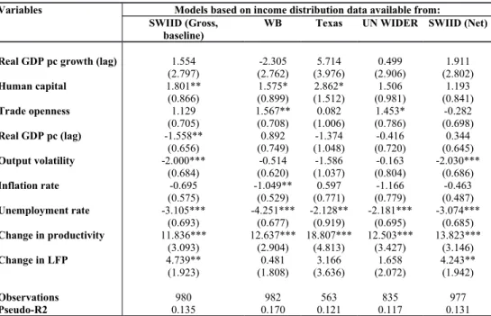
The analysis has so far used income distribution data available from SWIID to define the chronology of inclusive growth episodes. To test for the robustness of the empirical findings, we
estimated the baseline equation using different sources of income distribution data. The regression results, reported in Table 3, show that human capital accumulation, changes in multifactor productivity and the unemployment rate are robust across specifications. Moreover, the estimated coefficients are greater in magnitude for the chronology of inclusive growth episodes based on net income (after taxes and transfers) than on gross income (before taxes and transfers).
Table 3: Determinants of inclusive growth: Bivariate specification, alternative income distribution measures
Variables Models based on income distribution data available from:
SWIID (Gross, baseline)
WB Texas UN WIDER SWIID (Net)
Real GDP pc growth (lag) 1.554 -2.305 5.714 0.499 1.911
(2.797) (2.762) (3.976) (2.906) (2.802) Human capital 1.801** 1.575* 2.862* 1.506 1.193 (0.866) (0.899) (1.512) (0.981) (0.841) Trade openness 1.129 1.567** 0.082 1.453* -0.282 (0.705) (0.708) (1.006) (0.786) (0.698) Real GDP pc (lag) -1.558** 0.892 -1.374 -0.416 0.344 (0.656) (0.749) (1.048) (0.720) (0.645) Output volatility -2.000*** -0.514 -1.586 -0.163 -2.030*** (0.684) (0.620) (1.037) (0.804) (0.686) Inflation rate -0.695 -1.049** 0.597 -1.166 -0.463 (0.575) (0.529) (0.771) (0.779) (0.487) Unemployment rate -3.105*** -4.251*** -2.128** -2.181*** -3.074*** (0.693) (0.677) (0.919) (0.695) (0.685) Change in productivity 11.836*** 12.637*** 18.807*** 12.503*** 13.823*** (3.093) (2.904) (4.813) (3.427) (3.146) Change in LFP 4.739** 0.481 3.166 1.658 4.243** (1.923) (1.808) (3.636) (2.072) (1.942) Observations 980 982 563 835 977 Pseudo-R2 0.135 0.170 0.121 0.117 0.131
Note: All models are estimated by logit. Standard errors are reported in parenthesis. The constant term is omitted for parsimony. *, **, *** denote statistical significance at the 10, 5, and 1 percent levels, respectively. LFP denotes labor force participation.
Source: Authors’ estimations.
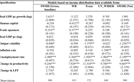
4.4. Evidence from multinomial probits
To shed further light on the empirical links between growth and income distribution, we re-estimated the baseline regressions by multinomial probit using the multivariate definition of inclusive growth and the corresponding chronology of episodes. The results, reported in Table 4, suggest that the growth channel is stronger than in the bivariate case, with lagged growth in real GDP per capita attracting a positively signed and statistically significant coefficient. The other regressors, except for human capital and real GDP per capita, remain as in the baseline specification. Also, as in the case of the regressions estimated by logit, the parameter estimates are higher in magnitude for the chronology
of inclusive growth episodes based on net income (after taxes and transfers) than on gross income (before taxes and transfers).
Table 4: Determinants of inclusive growth: Multinomial specification, alternative income distribution measures
Specification Models based on income distribution data available from:
SWIID (Gross, baseline)
WB Texas UN_WIDER SWIID (Net)
Real GDP pc growth (lag) 3.631* -3.122 3.370 0.765 1.901
(2.068) (2.251) (2.788) (2.145) (2.050) Human capital -0.234 -0.412** -0.267 -0.092 0.169 (0.173) (0.197) (0.239) (0.193) (0.172) Trade openness 0.333** 0.377** 0.255 0.198 0.297** (0.141) (0.188) (0.228) (0.188) (0.141) Real GDP pc (lag) 0.012 -0.018 0.059 -0.030 -0.014 (0.029) (0.034) (0.040) (0.031) (0.029) Output volatility -0.840* -0.594 -1.379** -0.632 -1.236*** (0.449) (0.469) (0.631) (0.496) (0.445) Inflation rate -0.536 -0.495 0.310 -1.396** -0.432 (0.381) (0.333) (0.418) (0.573) (0.359) Unemployment rate -2.480*** -3.364*** -1.926*** -1.964*** -2.189*** (0.497) (0.576) (0.613) (0.554) (0.494) Change in productivity 9.256*** 7.929*** 11.534*** 9.789*** 9.605*** (2.150) (2.289) (3.064) (2.420) (2.159) Change in LFP 2.716* -0.245 -2.789 0.766 2.200 (1.457) (1.441) (2.658) (1.542) (1.426) Observations 990 813 572 848 990
Note: Estimation by multinomial probit. Standard errors are reported in parenthesis. The constant term is omitted for parsimony. *, **, *** denote statistical significance at the 10, 5, and 1 percent levels, respectively. LFP denotes labor force participation.
Source: Authors’ estimations.
4.5. Using different sets of controls
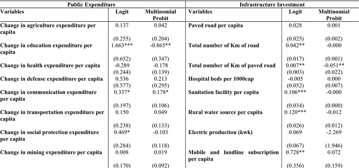
We augmented our baseline regression (using as before the SWIID measure of gross Gini as the dependent variable) with additional regressors, including public expenditure, infrastructure development, political and institutional factors, and indicators of financial development and financial crises. The estimation results are presented in three tables where only the coefficients of interest (for the variables introduced one at a time) are reported. The set of structural determinants is omitted for reasons of parsimony.21
Starting with public expenditure in Table 5, we confirm the importance of human capital as a driver of growth inclusiveness. Social protection also comes out with a positive and statistically
21 Full tables are available upon request. In general, the regressors remain signed as in the baseline specification and are statistically significance.
significant coefficient in the logit regression. Equally important is investment in transport and ICT. Indeed, when turning to infrastructure, the regression results show that the longer a country’s road network the more inclusive growth will tend to be. Sanitation facilities and water supply, proxying for better health conditions, are also important, at least as far as the logit regressions are concerned. Moreover, the number of landlines and mobile phone lines confirm the importance of ICT as a determinant of inclusive growth episodes.
Table 5: Determinants of inclusive growth: The role of public expenditure and infrastructure investment
Public Expenditure Infrastructure Investment
Variables Logit Multinomial
Probit
Variables Logit Multinomial
Probit Change in agriculture expenditure per
capita
0.137 0.042 Paved road per capita 0.028 0.001
(0.255) (0.204) (0.025) (0.002)
Change in education expenditure per capita
1.663*** -0.865** Total number of Km of road 0.042** -0.000
(0.652) (0.347) (0.017) (0.001)
Change in health expenditure per capita -0.289 -0.178 Total number of Km of paved road 0.007** -0.051**
(0.244) (0.139) (0.003) (0.022)
Change in defense expenditure per capita 0.536 0.213 Hospital beds per 1000cap -0.005 0.000
(0.577) (0.295) (0.052) (0.007)
Change in communication expenditure per capita
0.337* 0.178* Sanitation facility per capita 0.106*** -0.000
(0.197) (0.106) (0.034) (0.000)
Change in transportation expenditure per capita
0.150 0.049 Rural water source per capita 0.120*** -0.012
(0.238) (0.133) (0.026) (0.012)
Change in social protection expenditure per capita
0.469* -0.103 Electric production (kwk) 0.069 -2.269
(0.284) (0.118) (0.067) (1.946)
Change in mining expenditure per capita 0.008 0.019 Mobile and landline subscription
per capita 0.728** 0.072
(0.170) (0.092) (0.356) (0.159)
Note: The variables of interest are introduced one at a time in the baseline model. The remaining variables are omitted for economy of space. Standard errors are reported in parenthesis. *, **, *** denote statistical significance at the 10, 5, and 1 percent levels, respectively.
Source: Authors’ estimations.
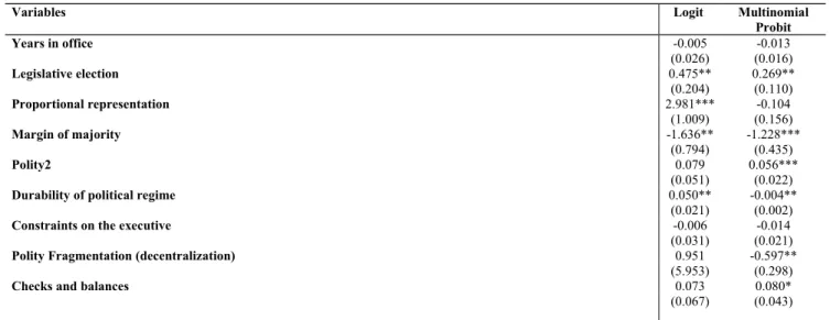
As far as the political and institutional factors ae concerned (Table 6), the regression results show that administrative continuity, at least as far as gauged by the number of years a government stays in office, does not seem to affect the probability of occurrence of an inclusive growth episode in a statistically discernible manner, but political stability, as reflected in the durability of a country’s political regime (at least as far as the logit regressions are concerned), does seem to matter. Also, having a healthy legislative environment characterized by electoral activity, as well as an electoral system based on proportional representation, positively affects the likelihood of an inclusive growth
episode. It is equally important that some degree of decentralization is in place to better reflect local demands and needs, at least as far as the multinomial probit regressions are concerned.
Table 6: Determinants of inclusive growth: The role of political and institutional factors
Variables Logit Multinomial
Probit Years in office -0.005 -0.013 (0.026) (0.016) Legislative election 0.475** 0.269** (0.204) (0.110) Proportional representation 2.981*** -0.104 (1.009) (0.156) Margin of majority -1.636** -1.228*** (0.794) (0.435) Polity2 0.079 0.056*** (0.051) (0.022)
Durability of political regime 0.050** -0.004**
(0.021) (0.002)
Constraints on the executive -0.006 -0.014
(0.031) (0.021)
Polity Fragmentation (decentralization) 0.951 -0.597**
(5.953) (0.298)
Checks and balances 0.073 0.080*
(0.067) (0.043)
Note: The variables of interest are introduced one at a time in the baseline model. The remaining variables are omitted for economy of space. Standard errors are reported in parenthesis. *, **, *** denote statistical significance at the 10, 5, and 1 percent levels, respectively.
Source: Authors’ estimations.
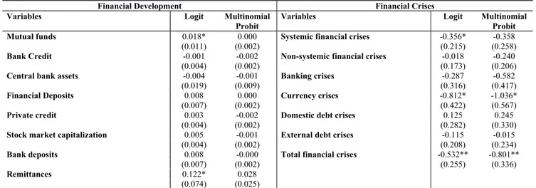
In Table 7, we turn to financial development and the occurrence of financial crises. The regression results are mixed, and most conventional proxies of financial development fail to attract statistically significant coefficients, with the exception of those related to the depth of mutual funds and reliance on remittances (in the logistic regression). As regards financial crises, systemic banking crises appear to have a more damaging effect on growth inclusiveness than non-systemic ones (in the logistic regression). Moreover, as expected, currency and financial crises seem to be particular detrimental to growth inclusiveness, regardless of the definition of inclusive growth episodes and estimator used.
Table 7: Logit and Multinomial Probit of Inclusive Growth: the role of financial development and financial crises
Financial Development Financial Crises
Variables Logit Multinomial
Probit
Variables Logit Multinomial
Probit
Mutual funds 0.018* 0.000 Systemic financial crises -0.356* -0.358
(0.011) (0.002) (0.215) (0.258)
Bank Credit -0.001 -0.002 Non-systemic financial crises -0.018 -0.240
(0.004) (0.002) (0.173) (0.206)
Central bank assets -0.004 -0.001 Banking crises -0.287 -0.582
(0.019) (0.009) (0.316) (0.417)
Financial Deposits 0.008 0.000 Currency crises -0.812* -1.036*
(0.007) (0.002) (0.422) (0.567)
Private credit 0.003 -0.002 Domestic debt crises 0.125 0.245
(0.004) (0.002) (0.282) (0.330)
Stock market capitalization 0.005 -0.001 External debt crises -0.115 -0.015
(0.004) (0.002) (0.208) (0.234)
Bank deposits 0.008 -0.000 Total financial crises -0.532** -0.801**
(0.007) (0.002) (0.255) (0.336)
Remittances 0.122* 0.028
(0.074) (0.025)
Note: The variables of interest are introduced one at a time in the baseline model. The remaining variables are omitted for economy of space. Standard errors are reported in parenthesis. *, **, *** denote statistical significance at the 10, 5, and 1 percent levels, respectively.
Source: Authors’ estimations.
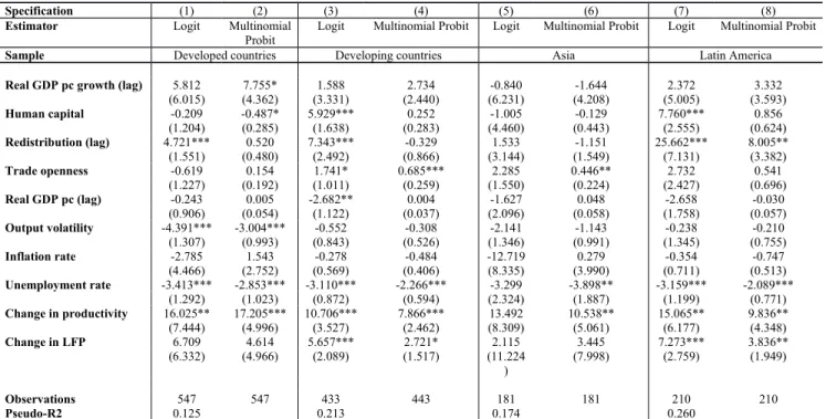
4.6. Analysis of sub-samples
We carried out an additional robustness check by splitting our sample along income and geographical lines and re-estimating the regressions by logit and multinomial probit. The results, reported in Table 8, show that the positive effects of human capital accumulation and trade openness are stronger in developing countries. On the other hand, the negative effect of output volatility on the probability of occurrence of an inclusive growth episode is stronger in the sub-sample of developed countries. Moreover, there are a few notable regional variations in the drivers of inclusive growth, with redistribution through the tax-benefit system, human capital accumulation and increases in labor force participation playing particularly important roles in Latin America, as compared to Asia.
Table 8: Determinants of inclusive growth: Split-sample analysis
Specification (1) (2) (3) (4) (5) (6) (7) (8)
Estimator Logit Multinomial
Probit
Logit Multinomial Probit Logit Multinomial Probit Logit Multinomial Probit
Sample Developed countries Developing countries Asia Latin America
Real GDP pc growth (lag) 5.812 7.755* 1.588 2.734 -0.840 -1.644 2.372 3.332
(6.015) (4.362) (3.331) (2.440) (6.231) (4.208) (5.005) (3.593) Human capital -0.209 -0.487* 5.929*** 0.252 -1.005 -0.129 7.760*** 0.856 (1.204) (0.285) (1.638) (0.283) (4.460) (0.443) (2.555) (0.624) Redistribution (lag) 4.721*** 0.520 7.343*** -0.329 1.533 -1.151 25.662*** 8.005** (1.551) (0.480) (2.492) (0.866) (3.144) (1.549) (7.131) (3.382) Trade openness -0.619 0.154 1.741* 0.685*** 2.285 0.446** 2.732 0.541 (1.227) (0.192) (1.011) (0.259) (1.550) (0.224) (2.427) (0.696) Real GDP pc (lag) -0.243 0.005 -2.682** 0.004 -1.627 0.048 -2.658 -0.030 (0.906) (0.054) (1.122) (0.037) (2.096) (0.058) (1.758) (0.057) Output volatility -4.391*** -3.004*** -0.552 -0.308 -2.141 -1.143 -0.238 -0.210 (1.307) (0.993) (0.843) (0.526) (1.346) (0.991) (1.345) (0.755) Inflation rate -2.785 1.543 -0.278 -0.484 -12.719 0.279 -0.354 -0.747 (4.466) (2.752) (0.569) (0.406) (8.335) (3.990) (0.711) (0.513) Unemployment rate -3.413*** -2.853*** -3.110*** -2.266*** -3.299 -3.898** -3.159*** -2.089*** (1.292) (1.023) (0.872) (0.594) (2.324) (1.887) (1.199) (0.771) Change in productivity 16.025** 17.205*** 10.706*** 7.866*** 13.492 10.538** 15.065** 9.836** (7.444) (4.996) (3.527) (2.462) (8.309) (5.061) (6.177) (4.348) Change in LFP 6.709 4.614 5.657*** 2.721* 2.115 3.445 7.273*** 3.836** (6.332) (4.966) (2.089) (1.517) (11.224 ) (7.998) (2.759) (1.949) Observations 547 547 433 443 181 181 210 210 Pseudo-R2 0.125 0.213 0.174 0.260
Note: Standard errors are reported in parenthesis. *, **, *** denote statistical significance at the 10, 5, and 1 percent levels, respectively. LFP denotes labor force participation.
Source: Authors’ estimations.
5. Conclusions
Inclusive growth episodes, at least as defined as growth in real GDP per capita that is not accompanied by a simultaneous deterioration in the distribution of income, are the outcome of a variety of socio-economic, policy and institutional factors. Overall, human capital accumulation, the redistributive potential of tax-benefit systems, increases in multifactor productivity and labor force participation, as well as trade openness and a range of institutional characteristics, including political system durability and electoral regimes, are powerful determinants of the probability of occurrence of an inclusive growth episode. As expected, economic volatility, inflation and joblessness are detrimental to growth inclusiveness. This cross-country evidence is fairly robust to the use of different estimators (including logit and multinomial probit), chronologies of inclusive growth episodes, data sources and sets of regressors.
From the point of view of policy design, the empirical findings are in line with mainstream thinking. They underscore the importance of redistribution through tax-benefit systems, human capital
accumulation and a sound macroeconomic framework. The main benefit of further empirical analysis in this area is the identification of those “win-win” or “super pro-poor” policy packages that would enhance growth together with distributive gains and also provide a better understanding of corrective measures when equity-efficiency trade-offs are identified.
By taking political and institutional characteristics into account, the analysis reported in this paper provides interesting insights for reform. While continuity is important, essentially because many pro-growth and distribution-friendly policies take time to bear fruit, it is not the durability of governments, but of political regimes, that seems to matter. Likewise, electoral systems also seem to affect the likelihood of growth inclusiveness, possibly in relation to the size of government, which tends to be larger under proportional representation than majority systems, therefore allowing for higher redistributive social spending. Although these linkages need to be tested further, the work pioneered by Persson et al. (2007), indeed shows that proportional representation induces a more fragmented party system and a larger incidence of coalition governments than majoritarian elections, resulting in larger governments.
References
1. Acemoglu, D., J.A. Robinson and T. Verdier (2012), “Why Can’t We All Be More Like Scandinavians? Asymmetric Growth and Institutions in an Interdependent World”, NBER Working
Paper, No. 1841, National Bureau of Economic Research, Cambridge, MA.
2. Ali, I. and H. H. Son (2007), “Measuring Inclusive Growth”, Asian Development Review, Vol. 24, pp. 11–31.
3. Anand, R., S. Mishra and S.J. Peiris (2013), “Inclusive Growth Revisited: Measurement and Determinants”, Economic Premise, No. 122, World Bank, Washington, D.C.
4. Andersen, T.M. and J. Maibom (2016), “The big trade-off between efficiency and equity: Is it there?”, CEPR Discussion Paper, No. 11189, Centre for Economic Policy Research.
5. Aoyagi, C. and Ganelli, G. (2015), “Asia’s quest for inclusive growth revisited”, Journal of
Asian Economics, Vol. 40, pp. 1–58.
6. Barro, R. J. and J. W. Lee (2013), “A new dataset of educational attainment in the world, 1950-2010”, Journal of Development Economics, Vol. 104, pp. 184–98.
7. Bartolini, D. and L. de Mello (2016), “Growth and Income Distribution: Does Decentralisation Matter?”, OECD, Paris, mimeo.
8. Beck, T., G. Clarke, A. Groff, P. Keefer and P. Walsh (2001, 2012), “New Tools in Comparative Political Economy: The Database of Political Institutions”, World Bank Economic
9. Berg, A. and J.D. Ostry (2011), “Inequality and Unsustainable Growth: Two Sides of the Same Coin?”, IMF Staff Discussion Note, No. 11/08, International Monetary Fund, Washington, D.C.
10. Bourguignon, F. (2003), “The Growth Elasticity of Poverty Reduction; Explaining
Heterogeneity across Countries and Time Periods”, in T. Eicher and S. Turnovsky (Ed.), Inequality
and Growth: Theory and Policy Implications (Cambridge, MA: MIT Press).
11. Brezzi, M. and L. de Mello (2016), “Inequalities in Latin America: Trends and Implications for Growth”, Hacienda Pública Española, forthcoming.
12. Brueckner, M. and D. Lederman (2015), “Effects of Income Inequality on Aggregate Output”,
World Bank Policy Discussion Paper, No. 7317, World Bank, Washington, D.C.
13. Cameron, A. C., and P. K. Trivedi (2005). “Microeconometrics: Methods and Applications”. New York: Cambridge University Press.
14. Causa, O., A. de Serres and N. Ruiz (2014), “Can Pro-Growth Policies Lift All Boats? An Analysis based on Household Disposable Income”, OECD Economics Department Working Papers, No. 1180, OECD, Paris.
15. Causa, O., M. Hermansen and N. Ruiz (2016), “The Distributional Impact of Pro-Growth Reforms”, OECD Economics Department Working Papers, No. 1342, OECD, Paris.
16. Cihák, M., A. Demirgüç-Kunt, E. Feyen, and R. Levine (2012), “Benchmarking Financial Systems around the World”, Policy Research Working Paper, No. 6175, World Bank, Washington, D.C.
17. Clarke, G.R.G. (1995), “More evidence on income distribution and growth”, Journal of Development Economics, Vol. 47, pp. 403–27.
18. de la Torre, A., J. Messina, and S. Pienknagura (2012) “The Labor Market Story Behind Latin America’s Transformation”, Semi-Annual Report, Regional Chief Economist Office, Latin America and the Caribbean, World Bank, Washington, D.C.
19. Deininger, K. and L. Squire (1998), “New Ways of Looking at on Old Issues: Inequality and Growth”, Journal of Development Economics, Vol. 10, pp. 565–591.
20. Dollar, D. and A. Kraay (2002), “Growth Is Good for the Poor”, Journal of Economic Growth, Vol. 7, pp. 195–225.
21. Dollar, D., T. Kleineberg and A. Kraay (2015), “Growth, Inequality and Social Welfare: Cross-Country Evidence”, Economic Policy, Vol. 30, pp. 335–77.
22. Ferreira, F., P. Leite and J. Litchfield (2007), “The Rise and Fall of Brazilian Inequality: 1981-2004”, Macroeconomic Dynamics, Vol. 12, pp. 1–32.
23. Galor, O. and J. Zeira (1993), “Income Distribution and Macroeconomics”, Review of
Economic Studies, Vol. 60, pp. 35–52.
24. Gao, S. and Shen, J. (2007), “Asymptotic properties of a double penalized maximum likelihood estimator in logistic regression”, Statistics and Probability Letters Vol. 77, pp. 925- 930.
25. Gasparini, L. and N. Lustig (2011) “The Rise and Fall of Income Inequality in Latin America”,
Working Paper, No. 2011-213, Society for the Study of Economic Inequality.
26. Gates, S. (2001), “Empirically assessing the causes of civil war.” Working paper (unpublished). 27. Greene, W. (2012), Econometric Analysis (Prentice Hall: New Jersey, N.J.).
28. Hermansen, M. N. Ruiz and O. Causa (2016), “The Distribution of the Growth Dividend”,
OECD Economics Department Working Papers, No. 1343, OECD, Paris.
29. King, G. (2001), “Proper Nouns and Methodological Propriety: Pooling Dyads in International Relations Data”, International Organization, Vol. 55, pp. 497-507.
30. King, G. and L. Zeng (1999a), “Logistic Regression in Rare Events Data”, Department of Government, Harvard University, Cambridge, MA.
31. King, G. and L. Zeng (1999b), “Estimating Absolute, Relative, and Attributable Risks in Case-Control Studies”, Department of Government, Harvard University, Cambridge, MA.
32. King, G. and L. Zeng (2001), “Explaining Rare Events in International Relations”,
International Organization, Vol. 55, pp. 693–715.
33. Kraay, A.(2004), “When Is Growth Pro-Poor? Cross-Country Evidence,” IMF Working Paper, No. 04/47, International Monetary Fund, Washington, D.C.
34. Laeven, L. and F. Valencia, (2010), “Resolution of Banking Crises: The Good, the Bad, and the Ugly,” IMF Working Paper, No. 10/44, International Monetary Fund, Washington, D.C.
35. Long, J. S., and J. Freese (2014). “Regression Models for Categorical Dependent Variables Using Stata”. 3rd ed. College Station, TX: Stata Press.
36. Lopez, H. (2004), “Pro-Growth, Pro Poor: Is There a Trade Off?”, Working Paper, No. WPS3378, World Bank, Washington, D.C.
37. Lopez, H. and L. Servén (2004), “The Mechanics of Growth-Poverty-Inequality Relationship”, World Bank, Washington, D.C., mimeo.
38. OECD (2015a), In It Together: Why Low Inequality Benefits All, OECD, Paris. 39. OECD (2015b), Going for Growth, OECD, Paris.
40. Ostry J., A. Berg and C. Tsangarides (2014), “Redistribution, Inequality, and Growth”, IMF
Staff Discussion Note, International Monetary Fund, Washington, D.C.
41. Persson, T., G. Roland and G. Tabellini (2007), “Electoral Rules and Government Spending in Parliamentary Democracies”, Quarterly Journal of Political Science, Vol. 20, pp. 1–34.
42. Ravallion (2001), “Growth, Inequality and Poverty: Looking Beyond Averages”, World
Development, Vol. 29, pp. 1803–15.
43. Reinhart, C. and K. Rogoff (2011), “From Financial Crash to Debt Crisis,” American
Economic Review, Vol. 101, pp. 1676–1706.
44. Tomz, M., G. King and L. Zeng, L. (1999), “Relogit Package”, Version 1.1.
45. Washington Centre for Equitable Growth (2015), “Fact sheet: What Do We Know About Inequality and Growth?”, July, 2015, Washington Centre for Equitable Growth, Washington, D.C. 46. White, H. and E. Anderson (2001), “Growth vs. Redistribution: Does the Pattern of Growth Matter?”, Development Policy Review, Vol. 19, pp. 267–89.
47. Wooldridge, J.M. (2002), Econometric Analysis of Cross Section and Panel Data, MIT Press, Cambridge, MA.
48. World Bank, (2005), Economic Growth in the 1990s: Learning from a Decade of Reform, World Bank, Washington, D.C.
49. Yu, B., Fan, S. and Magalhães, E. (2015), “Trends and composition of public expenditures: A global regional perspective”, European Journal of Development Research, Vol.27, pp. 353–370.
APPENDIX List of countries
Algeria, Angola, Argentina, Australia, Austria, Belgium, Bolivia, Brazil, Canada, Central African Republic, Chile, China, Colombia, Costa Rica, Cote Ivoire, Denmark, Dominican Republic, Ecuador, Egypt, El Salvador, Finland, France, Germany, Ghana, Greece, Guatemala, Honduras, Hungary, India, Indonesia, Ireland, Italy, Japan, Kenya, Korea, Malaysia, Mauritius, Mexico, Morocco, Netherlands, New Zealand, Nicaragua, Nigeria, Norway, Panama, Paraguay, Peru, Philippines, Poland, Portugal, Russia, Singapore, South Africa, Spain, Sri Lanka, Sweden, Switzerland, Thailand, Tunisia, Turkey, United Kingdom, United States, Uruguay, Venezuela, Zambia, Zimbabwe.
Summary Statistics
Variable Observations Mean Standard deviation Minimum Maximum Change in Gini SWIID gross 1,678 0.000964 0.034068 -0.19322 0.22744 Change in Gini World Bank 2,462 0.001345 0.041319 -0.74314 0.48023 Change in Gini Texas 1,125 0.005853 0.064182 -0.29741 0.277079 Change in Gini WIDER 1,384 0.001693 0.07487 -0.59782 0.438551 Change in Gini SWIID net 1,678 0.001769 0.027532 -0.1558 0.318969
Real GDP pc 5,280 10.58597 2.26132 5.535042 17.16027 Human capital 3,755 2.307359 0.591303 1.086181 3.618748 Redistribution 1,744 0.194321 0.203614 -0.21004 0.922655 Trade openness 4,334 0.790019 0.471394 0.003088 4.380917 Output volatility 4,508 0.313911 0.344533 0.002258 5.3846 Inflation rate 4,729 0.143202 0.366994 -1.29936 5.056657 Unemployment rate 2,170 8.846725 5.966464 0.154022 59.5 Productivity 4,248 22.6475 1.602984 18.82337 25.57951 Labor force participation 3,936 68.07909 10.28659 41 91.5
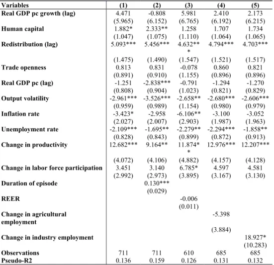
Table A1. Sensitivity to Inclusive Growth Episodes Strictly Longer than one year
Variables (1) (2) (3) (4) (5)
Real GDP pc growth (lag) 4.471 -0.808 5.981 2.410 2.173 (5.965) (6.152) (6.765) (6.192) (6.215) Human capital 1.882* 2.333** 1.258 1.707 1.734 (1.047) (1.075) (1.110) (1.064) (1.065) Redistribution (lag) 5.093*** 5.456*** 4.632** * 4.794*** 4.703*** (1.475) (1.490) (1.547) (1.521) (1.517) Trade openness 0.813 0.831 -0.078 0.860 0.821 (0.891) (0.910) (1.155) (0.896) (0.896) Real GDP pc (lag) -1.251 -2.838*** -0.791 -1.294 -1.270 (0.808) (0.904) (1.023) (0.821) (0.829) Output volatility -2.961*** -3.526*** -2.658** -2.680*** -2.606*** (0.959) (0.989) (1.154) (0.980) (0.979) Inflation rate -3.423* -2.958 -6.106** -3.100 -3.052 (2.027) (2.007) (2.903) (1.987) (1.963) Unemployment rate -2.109*** -1.695** -2.279** -2.294*** -1.858** (0.828) (0.843) (0.899) (0.872) (0.913) Change in productivity 12.682*** 9.164** 11.874* * 12.976*** 12.207*** (4.072) (4.106) (4.882) (4.157) (4.128) Change in labor force participation 3.451 3.140 6.785* 4.597 4.581
(2.992) (2.973) (3.895) (3.167) (3.130) Duration of episode 0.130*** (0.029) REER -0.006 (0.011) Change in agricultural employment -5.398 (3.884)
Change in industry employment 18.927*
(10.283)
Observations 711 711 610 685 685
Pseudo-R2 0.136 0.159 0.126 0.131 0.132
Note: All models are estimated by logit. Standard errors are reported in parenthesis. The constant term is not reported for parsimony. *, **, *** denote statistical significance at the 10, 5, and 1 percent levels, respectively.