António Afonso & João Tovar Jalles
Euro Area Time Varying Fiscal Sustainability
WP13/2015/DE/UECE _________________________________________________________
De pa rtme nt o f Ec o no mic s
W
ORKINGP
APERSE
URO AREA
T
IME VARYING
F
ISCAL
S
USTAINABILITY
*
António Afonso
$and João Tovar Jalles
Abstract
We assess the time varying features of fiscal sustainability in the euro area via revisiting the empirical relationship between the primary budget surplus and the debt-to-GDP ratio. Focusing on a sample of 11 Euro-area countries between 1999Q1 and 2013Q4 and by means of time series analyses, we find that: i) fiscal policy seems to have been sustainable in Belgium, France, Germany and Netherlands and a Ricardian (monetary dominant) regime might have been present; ii) debt exhibited a negative response following an innovation in the budget surplus in half of the sample; iii) the time-varying coefficient model shows that the 2008-2009 global economic and financial crisis exerted a sizeable negative impact on fiscal sustainability; iv) expenditure-based fiscal rules are strong determinants of fiscal sustainability. All in all, we found some evidence against the Fiscal Theory of the Price Level.
JEL: E62, H62, O52
Keywords: fiscal sustainability, causality, impulse response functions, time-varying coefficients, fiscal rules, logistic model
* The opinions expressed herein are those of the authors and do not necessarily reflect those of the authors’ employers.
$ ISEG/UL - University of Lisbon; UECE – Research Unit on Complexity and Economics. UECE is supported by FCT (Fundação
para a Ciência e a Tecnologia, Portugal), email: aafonso@iseg.utl.pt.
Center for Globalization and Governance, Nova School of Business and Economics Campus de Campolide 1099-032 Campolide,
2
1. INTRODUCTION
The relevance of fiscal developments for price behaviour and inflation can be traced back to some rather recent work linked to the so-called Fiscal Theory of the Price Level (FTPL), initially made popular by Leeper (1991), Sims (1994) and Woodford (1994, 1995). On the other hand, this discussion links further back to Sargent and Wallace (1975), and to the controversy of using rules to control the nominal interest rate, which may lead to price level indeterminacy. In a nutshell the main idea is that fiscal policy may have a relevant role, at least as important as monetary policy, in determining the price level.
Nevertheless, several authors argued against such theoretical possibility, notably McCallum (2001), and Buiter (2002). In addition, most available empirical assessments, provided by, for instance, Canzoneri, Cumby and Diba (2001), Cochrane (1998) and Woodford (1995), and Afonso (2008), point to the lack of adherence to the idea that price level may be determined via the intertemporal government budget constraint, given that governments are in fact quite Ricardian.
Weichenrieder and Zimmer (2014) also assess the euro area responsiveness of the primary balance
to government indebtedness. Therefore, the primary budget balance reacts to government debt to ensure fiscal solvency, implying the existence of an active monetary policy, and a passive fiscal policy.
In this paper we perform a systematic analysis of the relationship between the primary surplus and the debt-to-GDP ratio for a sample of 11 Euro-area countries using quarterly data between 1999Q1 and 2013Q4. In line with Bohn (1998) our approach provides an indirect test on the solvency of public finances and the exercise relies more specifically on the estimation of long-run cointegrating relationships as well as short-run Granger causality and impulse response function analyses. In addition to being the first paper to explore the sustainability question using quarterly data, we also include a novelty aspect which is to estimate country-specific time-varying coefficient models and use the resulting estimates to assess whether, within the EU fiscal framework, fiscal
rules act as important determinants for public finances’ solvency. Moreover, we also consider a logistic regression to assess if fiscal rules increase the likelihood of a sustainable fiscal policy.
3
exhibits a statistically significant negative response following an innovation in the budget surplus in half of the sample. Furthermore, the time-varying coefficient model uncovers the sizeable negative
impact to public finances’ sustainability of the global financial crisis, but also some reasons for
optimism going forward with the recovery process progressing satisfactorily. Finally, fiscal rules, expenditure-based in particular, are strong determinants of fiscal sustainability in our panel.
The remainder of the paper is organized as follows. Section 2 outlines the empirical framework and addresses data-related issues. Section 3 presents and discusses our main results. The last section concludes.
2. EMPIRICAL FRAMEWORK AND DATA
The idea of non-Ricardian regimes rests on the hypothesis that primary budget balances could be determined by the government without taking into account the level of government debt. In that vision of the world, money and prices would then need to adjust to the level of government debt to guarantee the fulfilment of the government intertemporal budget constraint, a passive monetary policy. Therefore, in the context of a non-Ricardian regime, the fiscal authority may autonomously decide on the budget balance and government debt, influencing the determination of the price level, while the monetary authority would, rather unorthodoxly, set endogenously the money supply and taking the price level from the government budget constraint.
The literature has traditionally resorted to two approaches to test empirically for the FTPL: i) The backward looking approach (Bohn, 1998) which would imply that, in a Ricardian
regime1, an increase in the (lagged) level of debt would result in a higher primary surplus today;
ii) The forward looking approach (Canzoneri, Cumby and Diba, 2001) which would imply that, in a Ricardian regime, a larger primary surplus today would lead to a reduction in the future level of debt.
In this paper, we follow for the most part the first approach, even though we will also briefly resort, for the sake of robustness, to the second approach. That said, we aim to estimate the
1This is equivalent to an “active” monetary policy, being the determination of prices its nominal anchor; or a “passive”
4
cointegrating relationship between the primary surplus and the (lagged) level of debt (both expressed as ratios to GDP) via the following fiscal reaction function:
1
t t t
s b (1)
where bt is the government debt and st is the government primary balance. t satisfies standard assumptions of zero mean and constant variance.
For our empirical analysis, we focus on a sample of 11 Euro Area countries2 using quarterly data between 1999Q1 and 2013Q4. The primary budget balance (% GDP) and the government debt (% GDP) are retrieved from Eurostat via Datastream. As already mentioned, and to our knowledge, the use of quarterly data to assess fiscal sustainability in a panel framework has not been employed for the euro area, another contribution of our paper.
3. RESULTS
3.1 Unit Roots and Structural Breaks
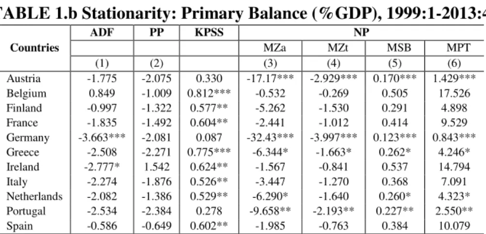
As a first step of the analysis, we investigate the time series properties of the primary surplus and debt series. Stationarity-wise, unit root tests can provide a valuable insight into the presence of either a deterministic or stochastic secular component in the series. In this context, in addition to standard Augmented Dickey Fuller (ADF) and Phillips-Perron (PP) unit root tests – for purposes of robustness and completeness3– we also conduct the four tests (M-tests) proposed by Ng and Perron (2001) (NP) based on modified information criteria (MIC): the modified Phillips-Perron test MZ; the modified Sargan-Bhargava test (MSB); the modified point optimal test MPT; and the modified Phillips-Perron MZT. These improve the PP-tests both with regard to size distortions and power.
The results are shown in Table 1a and 1b for the public debt and primary balance, respectively. We observe that the null hypothesis of non-stationarity cannot be rejected at the 10% level for the two series in most cases, independently of the test. Accordingly, both series would be I(1).
[Tables 1a, 1b]
2 The list of countries is: Austria, Belgium, Finland, France, Germany, Greece, Ireland, Italy, Netherlands, Portugal, and Spain.
5
We then resort to unit root tests allowing for breaks and we begin with the Zivot-Andrews (1992) (ZA) one. This endogenous structural break test is a sequential test which utilizes the full sample and uses a different dummy variable for each possible break date. The break date is selected where the t-statistic from the ADF test of unit root is at a minimum (most negative). We complement with the modified ADF test proposed by Vogelsang and Perron (1998) (VP) also allowing for one endogenously determined break. These test the null of unit root against the break-stationary alternative hypothesis.
For the unit root tests that allow for one endogenously determined breaks it is assumed that the shift can be modelled by a dummy variable DUt 0 for t≤TB and for t>TB, where TB is the shift date (time break). In the time series literature, two generating mechanisms of shifts are distinguished, additive outlier (AO) and innovational outlier (IO) models. As discussed in Vogelsang and Perron (1998), who consider an unknown shift date situation, the AO framework may be preferable to the IO statistics, even if the Data Generating Process (DGP) is an IO process. Results in Table 2 suggest that, even after accounting for possible endogeneous breaks in the series of interest, the null of unit root against the break stationary alternative is not rejected in most cases.
[Table 2]
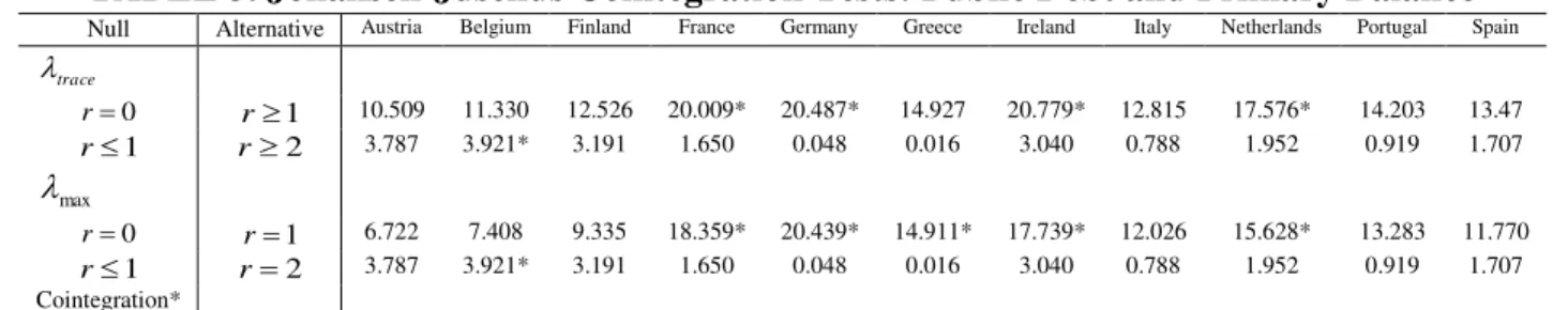
3.2 The Long Run: Cointegration and Stability
Given the nonstationarity of each individual time series, the relevant question becomes whether a linear combination of these two pairs of variables is stationary. If such a combination exists, government debt and primary balance become cointegrated, which implies that the variables are attracted to a stable long-run (equilibrium) relation and any deviation from this relation reflected short-run (temporary) disequilibria. We test for cointegrating relations between primary balance and government debt using the Johansen-Juselius methodology. This approach estimates the long-run attracting set in a VAR context that incorporates both the short- and long-run dynamics of the various models. According to Table 3 cointegration is found in Belgium, France, Germany, Greece, Ireland and Netherlands.
[Table 3]
6
providing a robust correction to the possible presence of endogeneity in the explanatory variable, as well as of serial correlation in the error terms of the OLS estimation. Hence, we first estimate a long-run dynamic equation including leads and lags of the (first difference) explanatory variable
and then perform Shin’s (1994) test from the calculation of C a LM statistics from the DOLS residuals which tests for deterministic cointegration, i.e., when no trend is present in the regression.
The results of the estimation of Equation (1) for each country, in terms of the coefficient and the statistic C appear in Table 4 (where leads and lags of the first difference of the explanatory variable were included). Results are twofold: first, since all but four of the cointegration statistics are not statistically significant, the null of deterministic cointegration is not rejected in those cases; and second, the estimates of are always positive and significantly different from zero at 10% level in four countries, namely Belgium, France, Germany and Netherlands. For these countries fiscal policy would have been sustainable and a Ricardian or MD regime would have prevailed. This is in line with previous contributions that analyze the case of the EU but using annual data instead (e.g. Ballabriga and Martinez-Mongay, 2003, 2005; Afonso, 2008). One caveat here relates to the fact that fiscal authorities might not have behaved in a linear fashion so that fiscal solvency might have hold in some periods for the set of countries not mentioned above.4
[Table 4]
Next we examine the possibility of instabilities in the cointegration relationship. As emphasized by Bruggemann et al. (2003), it is of some importance to formally investigate the stability of the cointegrating vectors further, once a long-run relationship has been identified. The temporal stability of estimated relations is also indicative of the usefulness of these relations for policy (forecasting) purposes. Hansen and Johansen (1993) outline a procedure that formally tests the constancy of cointegrating vectors in the context of Full Information Maximum Likelihood (FIML) estimations. Any rejection of the null of cointegration stability (constancy) should emanate from a breakdown in the long-run relation, rather than from any positive shift in the underlying short-run dynamics. We apply this approach to test the stability of the cointegrating relation. Results (shown
7
in the Appendix) suggest a stable relationship between the primary budget surplus and government gross debt.
3.3 The Short Run: Causality and Impulse Response Functions
A remark is worth making with respect to Equation (1): if a positive and significant coefficient is to be found that would be a sufficient condition for solvency, indicating that the government satisfies its present-value budget constraint. A problem with such finding is that it is compatible with both the MD and FD regimes.5 Hence, we will combine cointegration analysis with Granger-causality tests.
With this in mind, we employ Toda and Yamamoto (1995) approach for Granger causality. They suggest a technique that is applicable irrespective of the integration and cointegration properties of the system. The method involves using a Modified Wald statistic for testing the significance of the parameters of a VAR(l) model (where l is the lag length in the system). We follow Rambaldi and Doran (1996) in formulating these tests. Define dmaxas the maximum order of integration in the system, a VAR(kdmax) has to be estimated to use the Modified Wald test for linear restrictions on the parameters of a VAR(k) which has an asymptotic 2distribution. In our case, we will run a 2
variables’ VAR (for primary balance and (lagged) debt), with k=3 and dmax 1but for the sake of
notation simplicity, we denote them as ,y ii 1, 2,3. For our VAR(4) we estimate the following system of equations:
1
2
1 1 1 1 2 1 3 1 4
0 1 2 3 4
2 2 1 2 2 2 3 2 4
y
t t t t t
t t t t t y
e
y y y y y
A
y y y y y e
. (2)
The system in (2) is estimated via the seemingly unrelated regression (SUR) method. The test consists of taking the first k VAR coefficient matrix to make Granger causal inference. If, e.g., we want to test that y2tdoes not Granger-causey1t, the null hypothesis will be
(1) (2) (3) 0: 12 12 12 0
H , where ( ) 12 i
are the coefficients ofy2t i,i1, 2,3, 4.
5In a MD regime we would observe that an increase in previous’ period debt would lead to a larger primary balance ex
8
The results of the causality test for the variables under scrutiny are presented in Table 5. Bilateral short-run causality was found for Belgium, Germany and Ireland; whereas short-run causality just from debt to primary surplus appears for the Finland, France, Greece, Italy, Netherlands and Spain. The evidence for the latter set of countries suggests that a MD regime might have been present confirming the previous results from Table 4. Finally, no short run causality was found in any sense for Austria and Portugal.
[Table 5]
In order to provide a further robustness check, we discuss some additional results from the so-called forward-looking approach (Canzoneri, Cumby and Diba, 2001). We present the impulse response functions of the debt-to-GDP ratio to innovations in the primary surplus-to-GDP ratio, from an estimated VAR in these two variables. The VAR for each country was estimated with 4 lags and a constant (the optimal lag order was selected using the Akaike information criteria). The results are shown in Figure 1, together with one standard deviation bands. As can be seen, a general pattern appears: the debt to GDP ratio exhibits a statistically significant negative response following an innovation in the surplus-to-GDP ratio in Belgium, France, Ireland, Italy and Netherlands. Such response is increasing for a number of quarters and only in the case of France it becomes stable later on. This is in line with Melitz, (2000) who shows that fiscal policy has responded in a stabilizing manner for the EU-15 countries. In the remaining cases the response is generally negative but estimated with less precision.
[Figure 1] 3.4 Time-Varying Coefficient Model Estimation
The next step is to try to uncover the underlying movements in the coefficient represented in Equation (1). That is, we assess how has the so-called fiscal sustainability (or unsustainability) parameter of interest changed over time in each country under scrutiny. The model considered here generalizes the standard linear regression model by introducing the assumption that the regression coefficients may vary over time. Hence, with
1,𝑡 denotes the value of the coefficient belonging to
the first variable at time t,
2,𝑡 for the second coefficient, and so forth:
𝑦𝑡 = 𝑥1,𝑡1,𝑡+ 𝑥2,𝑡 2,𝑡+ 𝑥3,𝑡 3,𝑡+ ⋯ + 𝑢𝑡 (3)
with
9
𝑦𝑡 = 𝑥𝑡′ 𝑡+ 𝑢𝑡 . (4)
Regarding the coefficients , we assume that they change slowly and unsystematically over
time (random walk) in the sense that the expectation of today’s coefficient
𝑡 is equal to
yesterday’s state
𝑡−1. The change of coefficient i – its disturbance – from period t-1 to period t is
denoted by 𝑣𝑖,𝑡. It is assumed to be normally distributed with expectation zero and variance 𝜎𝑖2. With the vector of disturbances at time t denoted by 𝑣𝑡 = (𝑣1,𝑡, 𝑣2,𝑡, … , 𝑣𝑛,𝑡)′ we write:
𝑡= 𝑡−1+ 𝑣𝑡.
6 (5)
The variances 𝜎2 and (𝜎12, 𝜎22, … , 𝜎𝑛2) are calculated by a method-of-moments estimator that coincides with the maximum-likelihood estimator for large samples but is statistically more efficient and numerically more transparent and straightforward to interpret in small samples (see Schlicht, 1985, 1988). 7 The matrix of the estimated coefficients ̂ is obtained as the expectation of
given that data X and y’:
̂ = 𝐸{|𝑋, 𝑦}. (6)
Allowing to be time-varying and running the above model yields the country patterns displayed in Figure 2. A common pattern across the different charts is the impact of the global economic and financial crisis between 2008 and 2009 in changing the sign of the time-varying coefficient from positive to negative in the cases of Austria, Belgium, Finland, Ireland, Italy, Netherlands and Spain. In the remaining countries the sudden drop in magnitude is also visible even if the sign does not change. Moreover, the effect of the recovery and initial ease on public finances’ burden can be seen in most cases between 2010 and 2011. That said, only Germany managed to keep a positive estimated coefficient, that is, fiscal policies remained sustainable throughout the whole period.
[Figure 2]
6 The model (3), (4) generalizes the classical regression model. If the variances of the disturbances in the coefficients
(𝜎12, 𝜎22, … , 𝜎𝑛2) got to zero, the classical regression model is obtained as a special case.
7 The Varying-Coefficient model is statistically superior because it is a two-sided filter, whereas the alternative
Kalman-Bucy filter is, by construction, one sided. As a consequence, the estimate of the state of coefficients 𝑡 at time t will depend, in the Kalman-Bucy case, only on past and current but not on future observations. But the current state is correlated with future states and future observations will provide information about the current state. Hence, it is inefficient to use a one sided filter. Furthermore, and as a consequence of this, the initial state
10 3.5 Do fiscal rules help sustainability?
In order to try to understand, under the EU fiscal framework, what can help sustaining a sound path for public finances, we take the time-varying estimates as our dependent variable and regress it (using as weights the inverse of the standard errors of the ’s) against several fiscal rules (retrieved from the IMF’s Fiscal Rules dataset8). To this end, we rely on the number of existing numerical rules and then more specifically on expenditure-type and revenue-type rules.
We go one step further by considering a logistic regression in assess if fiscal rules increase the likelihood of a sustainable fiscal policy. More specifically, we consider the direct impact of fiscal rules (rules) and estimate the following model:9
Prob(sustainable 1|rules) ( i rules), (7)
where denotes the parameter to be estimated and () is the logistic function.10 Given that we rely on panel data, the structural model can be written as:
* it
* it it
sustainable rules ,
sustainable 1 if 0, and 0 otherwise. i it it
(8)
with i = 1, …, 11; t = 1999Q1, …, 2013Q4; itdenotes the country-specific time-varying slope coefficients estimated from Section 3.4; i captures the unobserved individual effects; and it is the error term.
The results from both regressions are shown in Table 6. We observe that the simple existence of fiscal rules if positively associated with a higher time-varying sustainability coefficient. Moreover, the more rules the higher the probability that the time-varying coefficient is positive. These results hold particularly strongly for expenditure-based rules, therefore reinforcing the need to have these mechanisms in place to avoid public finances to more easily get into an unsustainable path.
[Table 6]
8 http://www.imf.org/external/datamapper/fiscalrules/map/map.htm.
9 For details on this binary choice model see, for example, Greene (2012, Ch. 17).
11
4. CONCLUSION
In this paper we revisited the fiscal sustainability question by systematically analysing the relationship between the primary surplus and the debt-to-GDP ratio. Focusing on a sample of 11 Euro-area countries, using quarterly data between 1999Q1 and 2013Q4 and by means of cointegration, Granger-causality and impulse response function analyses, we found that: i) fiscal policy seems to have been sustainable in Belgium, France, Germany and Netherlands and, moreover, a Ricardian or monetary dominant regime might have been present in those countries (for the remainder of the countries in the sample no firm conclusion could be drawn); ii) debt exhibited a statistically significant negative response following an innovation in the budget surplus in half of the sample; iii) the time-varying coefficient model exercise uncovers the sizeable negative impact to
public finances’ sustainability of the global financial crisis, but also some reasons for optimism
going forward with the recovery process progressing satisfactorily; iv) fiscal rules, expenditure-based in particular, are strong determinants of fiscal sustainability in our panel.
12
REFERENCES
1. Afonso, A. (2008). “Ricardian Fiscal Regimes in the European Union”, Empirica, 35 (3), 313–334. 2. Bajo-Rubio, O., Diaz-Roldan, C., Esteve, V. (2004), “Searching for threshold effects in the evolution of budget deficits: an application to the Spanish case”, Economics Letters, 82, 239-243.
3. Bajo-Rubio, O., Diaz-Roldan, C., Esteve, V. (2006), “Is the budget deficit sustainable when fiscal policy is non-linear? The case of Spain”, Journal of Macroeconomics, 28, 596-608.
4. Ballabriga, F., Martinez-Mongay, C. (2003), “Has EMU shifted monetary and fiscal policies?” in Buti, M. (ed),Monetary and Fiscal Policies in the EMU, Interactions and Coordination, Cambridge University Press, Cambridge.
5. Ballabriga, F., Martinez-Mongay, C. (2005), “Sustainability of EU public finances”, Economic Paper 225, European Commission, DG Economics.
6. Bohn, H. (1998), “The behavior of U.S. public debt and deficits”,Quarterly Journal of Economics
113, 949–963.
7. Bruggemann, A., P. Donati and A. Warne (2003) Is the demand for euro area M3 stable?. ECB Working Paper No. 255
8. Buiter, W. (2002). “The Fiscal Theory of The Price Level: A Critique,” Economic Journal, 112 (481), 459-480.
9. Canzoneri, M.; and Diba, B. (1996). “Fiscal Constraints on Central Bank Independence and Price Stability,” CEPR Discussion Paper 1463.
10. Canzoneri, M.; Cumby, R and Diba, B. (2001). “Is the Price Level Determined by the Needs of Fiscal Solvency?” American Economic Review, 91(5), 1221-1238
11. Christiano, L. and Fitzgerald, T. (2000). "Understanding the fiscal theory of price level," Federal Reserve Bank of Cleveland. Economic Review, 2nd quarter, 2-38.
12. Cochrane, J. (1998). “Long-term Debt and Optimal Policy in the Fiscal Theory of the Price Level,” NBER Working Paper 6771.
13. Greene, W. H., 2012. Econometric Analysis. Prentice Hall, Upper Saddle River, NJ.
14. Hansen, H., and S. Johansen (1993), “Recursive estimation in cointegrated VAR models”, Preprint 1, Institute of Mathematical Statistics, University of Copenhagen.
15. Leeper, E. (1991). “Equilibria Under 'Active' and 'Passive' Monetary and Fiscal Policies,” Journal of Monetary Economics, 27 (1), 129-147.
16. McCallum, B. (2001). “Indeterminacy, Bubbles, and the Fiscal Theory of Price Level Determination,” Journal of Monetary Economics, 47 (1), 19-30.
17. Melitz, J. (2000), “Some cross country evidence about fiscal policy behaviour and consequences for EMU”, European Economy, Reports and Studies, 2, 3-21.
18. Ng, S., and P. Perron (2001). “Lag Length Selection and the Construction of Unit Root Tests with Good Size and Power,” Econometrica, 69, 1519-1554.
19. Rambaldi, A. N. and Doran, H. E. (1996) Testing for Granger non-causality in cointegrated systems made easy, Working Papers in Econometrics and Applied Statistics, Department of Econometrics, The University of New England, No.88, 22 pages.
13
21. Schlicht, E., 1985, Isolation and Aggregation in Economics, Berlin-Heidelberg-New York-Tokyo: Springer-Verlag.
22. Schlicht, E., 1988, “Variance Estimation in a Random Coefficients Model,” paper presented at the Econometric Society European Meeting Munich 1989.
23. Shin Y. 1994. A residual-based test of the null of cointegration against the alternative of no cointegration. Econometric Theory 10: 91–115.
24. Sims, C. (1994). “A Simple Model for the Study on the Determination of the Price Level and the Interaction of Monetary and Fiscal Policy,” Economic Theory, 4 (3), 381-399.
25. Stock, J. H. and M. W. Watson, 1993, “A simple estimator of cointegrating vectors in higher order integrated systems,” Econometrica, 61, 4, July, 783-820.
26. Toda, H.Y., and T. Yamamoto (1995) ‘Statistical inference in vector autoregression with possibly integrated processes.’ Journal of Econometrics 66, 225-250
27. Vogelsang, T.J., 2001. Testing for a shift in trend when serial correlation is of unknown form. Manuscript, Department of Economics, Cornell University.
28. Vogelsang, T.J., Perron, P., 1998. Additional tests for a unit root allowing the possibility of breaks in the trend function. International Economic Review 39, 1073-1100.
29. Weichenrieder, A., Zimmer, J. (2014). “Euro membership and fiscal reaction functions”,
International Tax and Public Finance, 21, 598–613.
30. Woodford, M. (1994). “Monetary Policy and Price Level Determinacy in a Cash-in-Advance Economy,” Economic Theory, 4 (3), 345-380.
31. Woodford, M. (1995). “Price Level Determinacy without Control of Monetary Aggregate,”
Carnegie-Rochester Conference Series on Public Policy, 43 (1), 1-46.
32. Wooldridge, J. (2002), Econometric Analysis of Cross Section and Panel Data, MIT Press.
14
TABLE 1.a Stationarity: Public Debt (%GDP), 1999:1-2013:4
Countries
ADF PP KPSS NP
MZa MZt MSB MPT
(1) (2) (3) (4) (5) (6)
Austria -1.105 -2.829* 0.335 -5.20 -1.411 0.271 5.216
Belgium -1.477 -2.290 0.501** -2.700 -1.135 0.420 8.974
Finland -1.109 -0.659 0.311 -2.267 -0.884 0.389 9.583
France 0.956 1.344 0.842*** -0.081 -0.034 0.428 15.669
Germany -0.457 -0.539 0.782*** 0.412 0.325 0.789 40.964
Greece 0.458 0.724 0.724** 0.846 0.423 0.500 22.070
Ireland -0.686 1.392 0.638** -30.52*** -3.760*** 0.123*** 1.248***
Italy -0.367 0.624 0.509** -23.207*** -3.231*** 0.139*** 1.638***
Netherlands 0.186 -0.206 0.591** -0.310 -0.172 0.554 20.627
Portugal 2.812 2.812 0.793** 3.080 4.035 1.309 163.61
Spain 0.194 1.112 0.397* -8.806** -1.851* 0.210** 3.688*
Note: ADF critical values: -4.028, -3.445, -3.145 for 1, 5 and 10% levels respectively. For the Ng-Perron test (NP), none of the test statistics are significant at the usual levels. The critical values are taken from Ng and Perron (2001), table 1 and the autoregressive truncation lag (zero) has been selected using the modified AIC. The null is of unit root.
TABLE 1.b Stationarity: Primary Balance (%GDP), 1999:1-2013:4
Countries
ADF PP KPSS NP
MZa MZt MSB MPT
(1) (2) (3) (4) (5) (6)
Austria -1.775 -2.075 0.330 -17.17*** -2.929*** 0.170*** 1.429***
Belgium 0.849 -1.009 0.812*** -0.532 -0.269 0.505 17.526
Finland -0.997 -1.322 0.577** -5.262 -1.530 0.291 4.898
France -1.835 -1.492 0.604** -2.441 -1.012 0.414 9.529
Germany -3.663*** -2.081 0.087 -32.43*** -3.997*** 0.123*** 0.843***
Greece -2.508 -2.271 0.775*** -6.344* -1.663* 0.262* 4.246*
Ireland -2.777* 1.542 0.624** -1.567 -0.841 0.537 14.794
Italy -2.274 -1.876 0.526** -3.447 -1.270 0.368 7.091
Netherlands -2.082 -1.386 0.529** -6.290* -1.640 0.260* 4.323*
Portugal -2.534 -2.384 0.278 -9.658** -2.193** 0.227** 2.550**
Spain -0.586 -0.649 0.602** -1.985 -0.763 0.384 10.079
Note: vide Table 1.a
TABLE 2. Stationarity and Structural Breaks: Public Debt (%GDP), 1999:1-2013:4
Public Debt Primary Balance
Countries ZA VP(AO) VP(IO) ZA VP(AO) VP(IO)
(1) (2) (3) (4) (5) (6)
Austria -6.593*** 6.155 2.703 -3.384 -1.906 -2.456
Belgium -5.462** 0.633 0.826 -5.951*** -5.056** -2.387
Finland -3.689 7.181 4.117 -4.049 -4.567** -5.287**
France -3.685 11.304 3.786 -4.386 -9.018** -4.793**
Germany -3.056 12.529 4.349 -4.646 -2.043 -2.771
Greece -4.174 16.583 3.969 -5.622*** -7.201** -5.127**
Ireland -3.622 17.102 5.487 -3.596 -1.072 -3.450
Italy -4.793 11.972 3.712 -3.318 -1.921 -1.840
Netherlands -6.876 11.568 6.589 -3.515 -4.546** -5.354**
Portugal -4.808 8.990 3.891 -4.581 -2.647 -4.776**
Spain -5.417** 6.910 2.818 -3.360 -5.207** -3.444
15
TABLE 3. Johansen-Juselius Cointegration Tests: Public Debt and Primary Balance
Null Alternative Austria Belgium Finland France Germany Greece Ireland Italy Netherlands Portugal Spain
trace
0
r r1 10.509 11.330 12.526 20.009* 20.487* 14.927 20.779* 12.815 17.576* 14.203 13.47 1
r r2 3.787 3.921* 3.191 1.650 0.048 0.016 3.040 0.788 1.952 0.919 1.707
max
0
r r1 6.722 7.408 9.335 18.359* 20.439* 14.911* 17.739* 12.026 15.628* 13.283 11.770 1
r r2 3.787 3.921* 3.191 1.650 0.048 0.016 3.040 0.788 1.952 0.919 1.707
Cointegration*
Note: * denotes rejection of the null hypothesis of no cointegration at the 5% level (based on MacKinnon-Haug-Michelis p-values).
TABLE 4. Estimation of long-run cointegration: Stock-Watson-Shin
DOLS
Country\relation C 2
R
Austria 0.578 0.010 0.131
(12.521) (0.183)
Belgium 12.58** 0.152*** 0.595
(5.327) (0.053)
Finland 1.113 0.077 0.551
(5.275) (0.128)
France 5.948*** 0.096*** 0.834
(1.444) (0.022)
Germany 8.161** 0.127** 0.431
(3.302) (0.049)
Greece 5.369 0.031 0.302
(6.542) (0.060)
Ireland 4.278 0.136 0.772
(3.235) (0.086)
Italy 4.868 0.059 0.479
(7.428) (0.067)
Netherlands 15.814*** 0.296*** 0.810
(3.135) (0.058)
Portugal 3.011 0.017 0.100
(3.481) (0.056)
Spain 3.492 0.061 0.870
(3.103) (0.062
Note: The C is the Shin (1994) LM statistic which tests for deterministic cointegration. The critical values are taken from Shin (1994), Table 1, for m=1. Standard errors in parentheses, adjusted for long-run variance. The long-run variance of the cointegrating regression residuals was estimated using the Barlett window with 6 ( 1/2)
T INT
l as proposed by Newey and West (1987). The number of leads and lags selected wasq4. *, ** and *** denote significance at 10, 5 and 1% levels, respectively.
TABLE 5. Causality tests – Public Debt and Primary Balance
Toda-Yamamoto
Country/direction
1
t t
s b Yes/No bt1st Yes/No
Austria 1.231 NO 6.341 NO
Belgium 11.44** YES 22.59*** YES
Finland 2.997 NO 18.202*** YES
France 0.544 NO 49.84*** YES
Germany 16.89*** YES 8.347* YES
Greece 3.008 NO 14.92*** YES
Ireland 39.325*** YES 20.631*** YES
Italy 2.047 NO 26.613*** YES
Netherlands 3.334 NO 43.55*** YES
Portugal 4.346 NO 6.184 NO
Spain 1.651 NO 28.722*** YES
16
TABLE 6. Weighted-Least Squares and Logistic Estimation: Fiscal Rules as determinants of Sustainability
(1) (2) (3) (4) (5) (6)
Regressors/Estimation WLS Logistic
Number of Numerical Rules 0.0134** 0.346***
(0.006) (0.054)
Expenditure Rule 0.039** 0.543***
(0.017) (0.011)
Revenue Rule 0.025* 0.206
(0.013) (0.649)
Observations 547 547 547 499 499 499
Adjusted-R2 0.289 0.291 0.288
log-likelihood -254.1 -265.1 -259.7
pseudo-R2 0.261 0.229 0.244
Notes: Estimation by weighted least squares (with weights the inverse of the standard errors of the estimated time varying coefficients – see text for details) and logistic regression. Standard errors in parentheses. *** p<0.01, ** p<0.05, * p<0.1. pseudo-R2=1-logL/logL0, where L is the likelihood of the model and L0 is the likelihood of the model without regressors. Throughout the various specifications, we include country fixed-effects. A constant term is also estimated but omitted.
Appendix
TABLE A1. Hansen Stability Test
Country Lc
Austria 0.008 (>0.2) Belgium 0.010 (>0.2) Finland 0.017 (>0.2) France 0.044 (>0.2) Germany 0.012 (>0.2) Greece 0.018 (>0.2) Ireland 0.029 (>0.2) Italy 0.012 (>0.2) Netherlands 0.014 (>0.2) Portugal 0.011 (>0.2) Spain 0.025 (>0.2)
17
Figure 1. Cumulative Impulse Responses based on individual country VARs
Austria -12 -10 -8 -6 -4 -2 0 2 4
1 2 3 4 5 6 7 8 9 10 11 12
Accumulated Response of LAGDEBT to Cholesky One S.D. PBAL Innovation
Belgium -25 -20 -15 -10 -5 0 5
1 2 3 4 5 6 7 8 9 10 11 12
Accumulated Response of LAGDEBT to Cholesky One S.D. PBAL Innovation
Finland -20 -16 -12 -8 -4 0 4
1 2 3 4 5 6 7 8 9 10 11 12
Accumulated Response of LAGDEBT to Cholesky One S.D. PBAL Innovation
France -5 -4 -3 -2 -1 0 1
1 2 3 4 5 6 7 8 9 10 11 12
Response of LAGDEBT to Cholesky One S.D. PBAL Innovation
Germany -24 -20 -16 -12 -8 -4 0 4
1 2 3 4 5 6 7 8 9 10 11 12
Accumulated Response of LAGDEBT to Cholesky One S.D. PBAL Innovation
Greece -80 -60 -40 -20 0 20 40
1 2 3 4 5 6 7 8 9 10 11 12
Accumulated Response of LAGDEBT to Cholesky One S.D. PBAL Innovation
Ireland -80 -70 -60 -50 -40 -30 -20 -10 0
1 2 3 4 5 6 7 8 9 10 11 12
Accumulated Response of LAGDEBT to Cholesky One S.D. PBAL Innovation
Italy -30 -25 -20 -15 -10 -5 0 5
1 2 3 4 5 6 7 8 9 10 11 12
Accumulated Response of LAGDEBT to Cholesky One S.D. PBAL Innovation
Netherlands -35 -30 -25 -20 -15 -10 -5 0 5
1 2 3 4 5 6 7 8 9 10 11 12
Accumulated Response of LAG_DEBT to Cholesky One S.D. PBAL Innovation
Portugal -36 -32 -28 -24 -20 -16 -12 -8 -4 0 4
1 2 3 4 5 6 7 8 9 10 11 12
Accumulated Response of LAGDEBT to Cholesky One S.D. PBAL Innovation
Spain -25 -20 -15 -10 -5 0 5
1 2 3 4 5 6 7 8 9 10 11 12
Accumulated Response of LAGDEBT to Cholesky One S.D. PBAL Innovation
18
Figure 2. Time Varying Coefficient Model Estimation
(plotting of slope coefficient estimates country-by-country, vertical axis)
Austria Belgium Finland
France Germany Greece
Ireland Italy Netherlands
Portugal Spain