Hedge Fund evaluation: mean variance vs performance ratios

(1)

Hedge Fund Evaluation:

Mean Variance vs Performance Ratios

Francisco Maria Morais David Everard do Amaral

Dissertation submitted as partial requirement for the conferral of Master in

Finance

Supervisor:

Prof. Luís Miguel da Silva Laureano, Assistant Professor, ISCTE-IUL Business School, Finance Department

(2)

(3)

I

Abstract

Combining the Mean Variance Utility function with the overall metrics that evaluate portfolios’ performance, this project aims to study the correlations of equal weighted portfolios based on the top 10 hedge funds of the studied sample, that maximize the expected utility of an investor and the performance measures; and to understand the overall results of the correlations between those portfolios.

Hedge funds are instruments that can represent different strategies, and in order to have an approximation to the different risk profiles, the correlations between the final ranks based on the different risk aversion coefficients in the Mean Variance Utility Function were studied. Constructing equal weighted portfolios with the top ten hedge funds that maximize the different levels of risk aversion, as well as the different performance metrics, the correlation between those portfolios will provide the final conclusion of the project.

These correlations proved that, since there are different types of investors that have different preferences, the process of evaluation of the portfolios cannot have the same methodology. Preferences should be taken in consideration, and there are metrics that are more correlated to the objectives of the final investor, than others.

JEL Classification: G11, G19

(4)

II

Resumo

Ao agrupar a função de utilidade média e variância com as mais conhecidas métricas que são utilizadas na avaliação de performance de portefólios, este projeto tem como objetivo estudar as correlações entre os portefólios, que maximizam as equações de utilidade média e variância, e os que maximizam as métricas de performance, tentado assim possibilitar uma conclusão sobre quais métricas que deverão ser utilizadas, ou que melhor representam as preferências de investidores com variados perfis de risco.

Os hedge funds são instrumentos que representam diferentes estratégias, e de forma a aproximar os diferentes perfis de risco, as correlações dos rankings que têm por base a maximização dos diferentes patamares de aversão ao risco na função de Média e Variância, foram estudadas.

Ao construir portefólios com base nos primeiros dez hedge funds, ponderados igualmente, que maximização as diferentes equações de Média Variância, traduzindo os diferentes perfis de risco, bem como os portefólios que maximizam as diferentes métricas que são utilizadas na avaliação de performance, o estudo das correlações destes portefólios irá proporcionar a conclusão final do projeto.

Estas correlações provam que, visto que existem diferentes tipos de investidores com diferentes preferências e objetivos, o processo de avaliação das diferentes performances não pode ter as mesmas metodologias. Estas preferências devem ser tidas em consideração, visto que existem métricas que são mais correlacionadas, do que outras, com os objetivos dos diferentes investidores.

(5)

III

Acknowledgement

I must thank to my supervisor Prof. Dr. Luís Laureano for his orientation and guidance since the very beginning of this project. Thanks to all my colleagues in Caixagest, specially David Yan and Pedro Frada, for their overall support, help and motivation during the last two years. Finally, I would also like to thank my family who are one of the most important people in my life, and more particular to my dear father, to whom I dedicate all the entire project.

(6)

Index

1. Sumário Executivo ... 1

2. Introduction ... 3

3. Literature Review ... 5

3.1 Modern Portfolio Theory ... 5

3.2 Expected Utility Theory (EUT) ... 7

3.3 Hedge Fund Performance ... 9

4. Data, Methodology and Sample Description ... 11

4.1 Data ... 11

4.2 Methodology ... 13

4.2.1 Performance Measures ... 13

4.2.2 Utility Function Approach... 18

4.3 Sample ... 20

5. Empirical Findings and Discussion ... 21

5.1 Risk Aversion Factor ... 21

5.2 Utility Rankings ... 22 5.2.1 Extreme Conservative ... 22 5.2.2 Conservative ... 23 5.2.3 Moderate ... 24 5.2.4 Moderate Aggressive ... 25 5.2.5 Aggressive ... 26

5.3 Performance Measures Ranking ... 28

5.3.1 Sharp Ratio ... 28

5.3.2 Sortino Ratio ... 29

(7)

5.3.4 Information Ratio ... 31

5.3.5 Maximum Drawdown ... 32

5.3.6 Modigliani and Modigliani ... 32

5.3.7 MAR Ratio ... 33 5.3.8 Skewness ... 34 5.3.9 Kurtosis ... 35 5.3.10 Standard Deviation ... 36 5.3.11 Excess Return ... 37 5.3.12 Cumulative Return ... 37 5.4 Correlations ... 41 6. Conclusions ... 44 7. Bibliography ... 46

Tables Index

Table 4-1 – Descriptive analysis of the Hedge Funds’ annualized return and standard deviation variables. ... 20

Table 5-1 – Aversion Factor Correlation Test between ranks ... 21

Table 5-2 – Rank obtained with Maximization of U with A=100 ... 22

Table 5-8 – Summary of The Portfolios’ Return and Standard deviation composed by the 10 Top Ranked Hedge Funds ... 27

Table 5-9 – Rank based on the maximization of Sharpe Ratio ... 28

(8)

Table 5-11 – Rank based on the maximization of Treynor Ratio ... 30

Table 5-12 – Rank based on the maximization of Information Ratio ... 31

Table 5-13 – Rank based on the maximization of Maximum Drawdown Ratio ... 32

Table 5-14 – Rank based on the maximization of M square Ratio ... 33

Table 5-15 – Rank based on the maximization of MAR Ratio ... 34

Table 5-16 – Rank based on the maximization of Skewness ... 34

Table 5-17 – Rank based on the maximization of Kurtosis ... 35

Table 5-18 – Rank based on the minimization of Standard Deviation ... 36

Table 5-19 – Rank based on the maximization of Excess Return ... 37

Table 5-20 – Rank based on the maximization of Cumulative Return ... 37

Table 5-21 – Measures that maximize a portfolio Annualized Return ... 38

Table 5-22 – Measures that minimize a portfolio Standard Variation ... 39

Table 5-23 – Overall correlation of the portfolios computed with the top 10 Hedge Funds that maximize each measure ... 41

Table 5-24 – Overall summary of the assessment to each of the risk profiles with the above 0.9 correlated performance measures utilized. ... 43

Figures Index

Figure 1-1 – Illustration of the Markowitz Efficient Frontier and the Tangency Portfolio ... 6

Figure 1-2 – Illustration of the Pascal Wager ... 8

Figure 5-1 – Accumulated Return over the 10y Period based on the several utility functions. ... 27

(9)

Equation Index

Sharpe Ratio ... 14 Treynor Ratio ... 14 Sortino Ratio... 15 Information Ratio... 15 Maximum Drawdown ... 15 M2 Ratio ... 16 Annualized Return ... 16

Annualized Standard Deviation ... 16

Excess Return ... 17

MAR Ratio ... 17

Skewness ... 17

Kurtosis ... 18

(10)

1

1. Sumário Executivo

A teoria moderna do portefólio teve o seu início em 1952, com o estudo de Harry Markowitz que defendeu que um portefólio eficiente deveria ter em consideração não só o retorno esperado como também o risco dos ativos que o compunham. A função de utilidade Média e Variância, ainda hoje é mundialmente conhecida e utilizada no estudo de portefólios, muito devido à sua simplicidade e fácil intuição. Dado que deriva da Teoria da Utilidade Esperada, que respeita um conjunto de axiomas estudados por John von Neumann e Oskar Morgenstern, é possível definir uma equação que traduza as preferências dos investidores.

O nascimento da Teoria Moderna Esperada começa na revolução marginalista, mas os conceitos por detrás da revolução remetem para séculos passados. O primeiro grande conceito aparece no século 17, por Blaise Pascal, através da Aposta de Pascal, que traduz a maximização do nível de utilidade esperado. Cem anos depois surgiu o segundo conceito que teve origem no paradoxo criado por Nicolaus Bernouli chamado São Petersburgo. Este paradoxo levou à criação e definição da lei de utilidade marginal decrescente. Finalmente, estes dois conceitos permitiram a Kenneth Arrow e John W. Pratt formularem um coeficiente que visa a traduzir o nível de aversão ao risco de cada investidor.

Combinando a mais importante literatura de avaliação da performance dos hedge funds, através das mais conhecidas métricas que são utilizadas na avaliação de performance e a função de utilidade de Média e Variância, este projeto propõe-se avaliar as correlações existente entre os diversos portefólios criados com base nestes dois ramos das finanças. O objetivo será o analisar quais métricas de performance é que deverão ser mais enfatizadas e utilizadas, na avaliação de hedge funds, para os diferentes perfis de risco.

O estudo das correlações dos rankings que maximizam a equação de Média e Variância possibilita identificar os diferentes coeficientes de aversão ao risco, caracterizando por isso o nível de tolerância à volatilidade e por consequente o perfil de risco. Desta forma é possível construir portefólios que caracterização as preferências dos investidores e compara-los com

(11)

2 os portefólios compostos pelos hedge funds que maximizam as diferentes métricas utilizadas na avaliação de performance.

A composição dos portefólios onde o estudo das correlações incide, tem por base diferentes

hedge funds com diferentes distribuições de retorno e consequentemente diferente

características. Por um lado os portefólios construídos maximizam níveis de utilidade representativos de perfis de risco, e por outro maximizam métricas de performance, mais utilizadas para premiar a estabilidade, o retorno, o tradeoff entre risco e retorno, entre outros…

Ao comparar os portefólios que têm por base, por um lado, o nível de utilidade que possibilita uma conclusão mais qualitativa, mas também por outro, os diferentes níveis de performance, possibilitando uma conclusão mais quantitativa, torna-se possível analisar o grau de efetividade das métricas de avaliação de performance quando utilizados no processo de avaliação.

Tendo por base um objetivo de investimento, um perfil de risco e um investidor com preferências definidas, a metodologia deve ir ao encontro dessas preferências. Ao efetuar o estudo das correlações entre os diferentes portefólios, é possível identificar quais são as métricas de avaliação de performance que são mais correlacionadas com os diferentes perfis de risco. Desta forma e tendo em consideração o facto de existirem diferentes tipos de investidores que têm diferentes objetivos, preferências e diferentes níveis de tolerância face ao risco, é necessário utilizar diferentes metodologias que têm por base uma decisão de investimento.

(12)

3

2. Introduction

Modern Portfolio Theory started in 1952, when Harry Markowitz defended that an efficient portfolio not only should consider the expected return, as well as the variance of the overall assets in it. Mean Variance equation came to be one of the most popular and discussed portfolio approaches, much related to its simplicity and intuition. Since it is a subclass of Expected Utility Theory, respecting a number of axioms defended by von Neumann and Morgenstern, it makes possible to translate the overall investors’ preferences.

Expected Utility Theory born during the marginal revolution, but its concepts emerged some time before. In the 17th_{century, Blaise Pascal, thought the very well-known Pascal Wager} and the concept of utility maximization, defended that a person could maximize his expected utility by believing in God. A century after Bernoulli gave birth to the second big concept of this theory with the famous St. Petersburg Paradox and consequently the law of diminishing marginal utility. These two concepts provided Kenneth Arrow and John W. Pratt with the mathematic definition of risk through risk aversion absolute coefficient.

Combining hedge fund evaluation and the most traditional performance metrics already known, with the main ideas behind Mean Variance utility function, this project aims to study the correlation between the portfolios selected based on these two different fields of finance. The first, more related to traditional finance and the second one related to behavioral finance. The objective will be to better know what metrics should be more emphasized in the evaluation of a hedge fund for the different risk profiles.

The study of correlations of the rankings that maximize Mean Variance equation makes it possible to identify the different risk aversion coefficients, characterizing therefore the level of tolerance to volatility and consequently the risk profile. This way it can be built portfolios that characterize the preferences of investors and comparing them with portfolios that maximize the different metrics used in evaluating performance.

The construction of the portfolios where the study of correlations focuses is based on a sample of different hedge funds with different return distributions and therefore different

(13)

4 characteristics. It is compared the portfolios that were built with the objective of utility maximization, representing risk profiles, and portfolios that maximize performance ratios, that are more used to reward stability, return, tradeoff between risk and return, among others...

By comparing the portfolios that are based on, first, the level of utility that enables a more qualitative conclusion, but also, different levels of performance, enabling a more quantitative conclusion, it becomes possible to analyze the degree of effectiveness of the performance evaluation metrics when used in the evaluation process.

Based on an investment purpose, a risk profile and well-defined investor’s preferences, the methodology should meet those objectives. When making the study of correlations between the different portfolios, it is possible to identify what are the performance evaluation metrics that are more correlated with different risk profiles. Thus, taking into account the fact that there are different types of investors that have different goals, preferences and different levels of risk tolerance, it must be used different methodologies that support the investment decision.

(14)

5

3. Literature Review

In this chapter will be reviewed the main concepts regarding the project. In the first section, since it will be used a Mean Variance utility function, the core ideas about the Modern Portfolio Theory will be analyzed. As the Mean Variance utility function is considered a subclass of Expected Utility Theory, the concepts regarding this theory will be also reviewed.

In the end and since the purpose is to compare the correlation between a mean variance utility function with some traditional performance measures and coefficients based on a sample of hedge funds, the latest aspects that this project will focus will be regarding hedge fund performance evaluation.

3.1Modern Portfolio Theory

Known as the father of the Modern Portfolio Theory, the Noble Prize award winner Harry Markowitz formulated the portfolio choice of the mean variance of assets. In summary, Markowitz (1952) proved that it is possible to, given a value of risk, measured by the standard deviation1_{, maximize the expected return of a portfolio; or in another perspective, that it is} possible, for a level of expected return, to minimize risk. These two principles led to the formulation of an efficient set of possibilities, frontier, from which the investor could choose an efficient portfolio, labeled in Figure 1-1 as “T”, positioned in the tangent to the frontier that depended on the investor risk return preferences (Elton and Grubber, 1997).

1_{“Measure of dispersion of a set of data from its mean. The more spread the data, the higher the deviation.}

Standard deviation is calculated as the square root of variance. In finance, standard deviation is applied to the annual rate of return of an investment to measure the investments’ volatility.”

(15)

6

Figure 1-1 – Illustration of the Markowitz Efficient Frontier and the Tangency Portfolio

Source: Lee and Su (2014)

Markowitz defended that an investor needed to consider the behavior of the securities in the portfolio, and the co-movements, or in other words, the covariance,2_{between all of them. If} investors considered the overall covariance it would lead to the construction of a portfolio that with the same expected return would have a minor level of risk than a portfolio that would not consider the interactions between all the securities (Elton and Grubber, 1997).

Since this represents a simplification, by just considering two moments, mean, or expected return, and variance, or risk, there were proposed some extensions to the Markowitz model.

First, Mandelbrot (1963) developed a model based on a logarithmic function. His opinion was that return distribution often revealed several outliers 3_{that weren’t taken in} consideration, stating that Markowitz’s model assumed normal return distribution.

Lee (1977), Kraus and Litzenberger (1976) recommended that skewness4_{and kurtosis}5 should be taken in consideration when estimating risk and return, because it would represent a more realistic representation of the return distribution.

Aside return distributions, more theoretical questions were raised analyzing how viable was to use a single period model, focusing in a multi-period investor problem. Mossin (1969),

2_{Measure of the degree to which returns on two risky assets move tandem. A positive covariance means that}

asset returns move together. A negative return means returns move inversely.

3_{Values that are smaller or larger than the most other values of the data.}

4_{Please see the definition given in Chapter 4, Data Methodology and Sample Description} 5_{Please see the definition given in Chapter 4, Data Methodology and Sample Description}

(16)

7 Fama (1970) and Merton (1971) showed under several assumptions, despite reaching to different optimal portfolios, that a multi-period problem could be solved as a sequence of several single-period problems.

Elton and Gruber (1997) concluded that despite everything written before, mean variance theory had “remained the cornerstone of modern portfolio theory” (Elton and Gruber 1997: 1745). It is full of insight about the preferences of investors and is recognized and used mainly for its simplicity, overall knowledge and intuition.

Ang (2014) refuted the idea that Mean Variance Theory assumed normal distributed returns. Despite just considering two moments, return and variance, that can lead to the misleading interpretation that it only takes in consideration normal distributions, Ang bases his conclusions on Levy and Markowitz (1979) that “showed that using mean-variance utility is

often a good approximation with non-normal returns” (Ang, 2014: 51).

3.2Expected Utility Theory (EUT)

EUT consists mainly in two concepts. The first concept is that an investor should use the expected value of utility to help him in the overall decision making process, and the second one is concerned with the concept of decreasing marginal utility6_.

The idea of market decision based on the maximization of expected utility goes back to the 17th_{century. In summary, Pascal (1670) presented an argument that states that believing in} God is rational and not believing is not rational, this idea is worldly known as Pascal Wager. Assessing any sets of probabilities, larger than 0, to the occurrence of the possible events, a consumer will have higher expected utility by believing in God as illustrated in figure 1-2 (Lengwiller, 2008).

6_{http://www.investopedia.com/terms/l/lawofdiminishingutility.asp - as a person increases the consumption of}

a product, keeping consumption of others constant, there is a decline in the marginal utility that a person derives from consuming each additional unit of that product. – access on

(17)

8

Figure 1-2 – Illustration of the Pascal Wager

Existence of God No Yes P er so n a l C o n d u ct R el ig io u s Finite Utility (-) Infinite Utility (+) S in fu l Finite Utility (+) Infinite Utility (-)

Source: Adapted from http://backyardskeptics.com/wordpress/pascals-wager/

Relatively to the second concept of diminishing marginal utility, it goes back to the 18th century with the insight given by Bernoulli (1713) and Cramer (1728). Nicolaus Bernoulli in 1713 formulated a problem, known as the St. Petersburg Paradox. This problem is related to probability and decision theory in economics. In summary, the paradox describes a casino that offers a reward for the simple game of tossing a coin. A player would win 2k, where k is equal to the number of tosses, until a head occurs. The question raised by Bernoulli was what should be the fair price for entering the game. Cramer (1728) as a response to Bernoulli proposed to evaluate gambles by considering the expected utility of the money gained, measured by the square root of the payoff. Bernoulli (1738), cousin of Nicolaus, proposed to use a logarithmic function, known as log utility, of the gamblers total wealth.

Menger (1934) refuted the idea of unbounded expected utility value, and stated that for more precise and convincing conclusions it was needed a bounded function. The axiomatization of the theory that was provided by von Neumann and Morgenstern (VNM) (1944) refutes also the idea of unbounded utility function (Lengwiller, 2008). VNM proved that if and only if the agent’s preferences respected four axioms7_{, than it would be possible to construct an}

7_{Completeness assumes that an individual has well defined preferences; Transitivity assumes that preferences}

(18)

9 utility function that always tried to maximize its expected value. In summary, “they proved

deductively that if decision-making is logical in the sense that it obeys certain specified basic axioms of coherence or rationality, then implicitly the decision-maker must act as if her objective is to maximize expected utility” (Johnstone and Lindley, 2013: 2).

In economics theses preferences assume that investors are risk averse. So, and relating to what have been reviewed before, this fact means that an investor has a positive but diminish marginal utility for money, or in mathematical terms, the utility function must be increasing and concave. Pratt and Arrow (1965) in the absolute measure of risk aversion capture the degree of concavity of utility or, in other terms, the rate at which marginal utility is decreasing at a given wealth (Johnstone and Lindley, 2013). Arrow (1965) concluded that “broadly

speaking the relative risk aversion must hover around 1, being, if anything, somewhat less for low wealths and somewhat higher for high wealths” (Arrow, 1965: 37).

Meyer (1987) “saw that MV offered a way of rewriting a subclass of expected utility that not

only simplified the notions of risk and return, but which also revealed previously unrecognized relationships between the risks and returns of individual assets and their combinations in weighted portfolios” (Johnstone and Lindley, 2013: 14).

3.3Hedge Fund Performance

The scientific discusses about Hedge Fund Performance is vast.

Géhin (2004) stated that there are several factors that characterize hedge funds and that all need to be considered in the process of evaluation. Géhin divides this matter in four sections. The first highlights the importance of the quality of the database; the second examines the return factors; the third part focus in the advantages and the drawbacks of traditional performance indicators, and a final section where he discusses performance models.

than and worse than a given middle option; Independence assumes that preferences holds independently of the possibility.

(19)

10 Elin, Farinelli, Rossello and Tibiletti (2009) analyzed a sample of 4048 hedge fund to understand the mismatch between the Sharpe Ratio and tailor-made ratios. Since the used ratios (Sortino-Satchell; Farinelli-Tibilletti and Rachev ratios) have parameters that allow some flexibility in the choice of which sector of the return distribution is more focused, it is possible to address more correctly the investor risk aversion profile. The study concluded that as long as tailor-made ratios describe moderate and conservative investment styles, the rank correlation with the Sharpe Ratio is closed to 1. But if investment styles were more aggressive the correlation were drastically reduced and the use of Sharpe Ration would become questionable.

Eling (2008) testes using a sample of more than 38 thousand funds, from 1996 to 2005, concludes that “Tests results indicate that the choice of any measure does not have significant

influence on the ranking of funds with different return distributions” (Hsieh and Hodnett,

2013: 821). Eling defends that Sharpe Ratio, is one of the best performance measure understood by investors, he considers that Sharpe Ratio “could also be considered superior

to the other performance measures” (Eling, 2008: 11) and has consistency with the expected utility maximization being extremely adequate in the evaluation of hedge funds.

Zakamouline (2009) proposes to refute Eling (2008) and Eling and Schumacher (2007) studies by stating that the choice of performance measures does influence the evaluation of hedge funds. He made theoretical, empirical and simulation analysis of rank correlations between alternative performance measures and Sharpe Ratio. In the first part he showed, addressing four reasons, why Elling and Schumacher were mistaken, and that the correlations between the Sharpe Ratio and alternative performance measures were “far from being

identical” (Zakamouline, 2009: 26). Adding to these conclusions Zakamouline states that

(20)

11

4. Data, Methodology and Sample Description

4.1Data

For this study, a sample of hedge funds was used. The risk free rate considered will be the 3 month US Libor Total Return, which will also be considered as a Benchmark. Hedge funds

“are alternative investments using pooled funds that may use a number of different strategies in order to earn active return, or alpha, for their investors. Hedge funds may be aggressively managed or make use of derivatives and leverage in both domestic and international markets with the goal of generating high returns (either in an absolute sense or over a specified market benchmark)”.8_{Benchmark is a “standard against which the performance of a security,}

mutual fund or investment manager can be measured”.9

Since Hedge Funds “invest in a heterogeneous range of financial assets (…) and cover a

wide range of strategies” (Géhin, 2004: 2), they have different return profiles which make

them a good instrument to analyze in order to be selected to different investors with different risk profiles.

The use of Bloomberg’s platform, through FRSC <GO> function, allowed to extract the Hedge Funds that were used in this study.

Of the available 573498 funds available in Bloomberg’s database and to serve the purpose of the study it was used the following criteria:

• Market Status……….. Active • Fund Primary Share Class……….. Yes • Fund Objective……….Alternative

• Fund Type………..Hedge Fund

• Currency………USD

• Inception Date……….Before 31-12-2004 • Fund Total Asset…………...Superior than 100M

8_{Hedge Fund - http://www.investopedia.com/terms/h/hedgefund.asp. Accessed on 5}th_{May 2015} 9_{Benchmark - http://www.investopedia.com/terms/b/benchmark.asp. Accessed on 5}th_{May 2015}

(21)

12 In order to analyze the hedge funds’ consistency and behavior in different financial market environments, the chosen period of analysis is the last 10 year (2005 – 2014). The overall financial markets in this period had sub periods where it can be seen a “bull” or an uptrend return distribution; “bear” or downtrend return distribution; and “trading range” or no trend return distribution.

Since 2014 is included in the sample, in order to have the most updated available data, all the hedge funds considered need to be currently active for investment.

To have a good sample with a wide variety of strategies, and return distributions, as explained before, only the “alternatives” and “hedge fund type” funds were considered.

To remove duplicate hedge funds, only were considered the primary share class. In order to reach every client globally, often asset companies create different share classes of the same hedge fund. Two of the possible reason to do it is the elimination of currency risk10_{, making} possible to invest in different currencies11_{, as well as, apply different levels of commission} between different types of clients12_.

Small funds often are oblige to deviate the core strategy due to a large concentration of clients. When these want to make a substantial redemption to the invested amount, managers need to sell positions in order to create the liquidity demanded. To eliminate the possibility of having return distributions that are not explained by strategy but by necessity of generating cash, only hedge funds bigger than 100 million dollars were considered. These funds have the needed monthly liquidity to not change the overall strategy of the fund and not lead to misinterpretation of the results.

10_{Change in price of a currency against another.}

11_{Asset companies distribute their funds in different currencies providing the overall hedging (immunization)}

of the currency risk.

12_{In order to differentiate clients, asset companies distribute the same fund to institutional clients that often}

invest larger amounts than retail clients. As the amounts invested are different the overall fee charged by the manager is different. To do so, asset manager companies create to different share classes that charge two different levels of commission.

(22)

13 In terms of currency, just the United States Dollar (USD) funds were considered since the United States is the country where there are more Hedge Funds available. In order to have a more homogenous sample, the other currencies were ignored since it would be needed to remove the performance of the currency in order to compare the overall hedge funds, and that is not the objective of the study.

The selected criteria provided a sample of 113 funds. In order to provide a more accurate conclusion, the top and bottom 2.5% Outliers in terms of return and standard deviation were excluded. Since these are the basis of the most performance indicators the inclusion of the top and bottom 2.5% could mislead the final conclusions

From the previous 113 Hedge Funds, and after eliminating the outliers, we obtain the final sample of 104 Hedge Funds.

The historical monthly past prices (net of fee) of every fund were studied, through the use of Bloomberg’s platform. The historical prices gave a notion of the return and risk (measured by the standard deviation).

4.2Methodology

4.2.1 Performance Measures

In terms of performance measurement several ratios (already known, and studied), that are used in the evaluation of the portfolios for one of the teams of my company were utilized: Sharpe ratio, is one of the most referenced risk adjusted measures in finance, and much of its popularity is due to its simplicity. This ratio measures the return in excess of the risk free rate (risk premium), comparing with the total risk of the portfolio measured by the standard deviation. In summary, it describes how much excess return receives for a unit of extra volatility and represents an attempt of measurement and prediction of mutual fund performance. The use of the Sharpe Ratio makes possible the comparison of different strategies and consequently different levels of risk, in an ultimate conclusion of portfolio management efficiency. The output of this ratio will give the added return that is received for the extra risk intake, of preferring the risky asset over the risk free asset.

(23)

14 Sharpe Ratio = (1)

Rp – Annualized Return of the Portfolio Rf – Annualized Return of the Risk Free rate σp – Standard Deviation of the Portfolio

Treynor (1965) developed a ratio that attempts to measure how well an investment has compensated its investors given a level of risk. When comparing to the Sharpe Ratio the main difference is the variable of discount the excess return. Treynor’s rely on beta. Beta is “considered a measure of volatility, or systematic risk of a security or portfolio in comparison

to the market as a whole. Beta is used in the Capital Asset Pricing Model (CAPM), a model that calculated the expected return of an asset based on its beta and expected market returns.” 13

Treynor Ratio = (2)

Rp – Annualized Return of the Portfolio Rf – Annualized Return of the Risk Free rate βp – Beta Coefficient of the Portfolio

Sortino (1983) developed this ratio based on the Sharpe Ratio, with the variant that the risk free rate is replace by a “minimum accepted threshold”, which in this study will be the return of the risk free rate, equally to the Sharpe Ratio, but instead of considering the overall standard deviation of the return distribution, only considers the standard deviation of the negative returns, creating the notion of good and bad volatility. Due to the limitations identified in Sharpe Ratio, that tends to punish the upside risk, the Sortino ratio proposes to

(24)

15 change the notion of risk by the negative semi-variance, ignoring the risk inherent to the volatility of upside movements.

Sortino Ratio =

(3)

Rp – Annualized Return of the Portfolio Rf – Annualized Return of the Risk Free rate

σ_D – Standard Deviation of the Negative Returns of the Portfolio

Information Ratio is a measure also known as appraisal ratio, and is defined by the residual return of the portfolio compared to its residual risk. It is the risk premium added by the portfolio manager, divided by the standard deviation of the risk premium itself. It shows the consistency of the fund manager in generating excess return when compared with the benchmark.14_{“Information ratio, (…) is useful for evaluating hedge funds that have an}

objective to achieve absolute returns as it measures the reward-to risk ratio of a portfolio against the performance of an explicit benchmark” (Hsieh and Hodnett, 2013: 821).

Information Ratio =

( ) (4)

Rp – Annualized Return of the Portfolio Rf – Annualized Return of the Risk Free rate σ(Rp-Rf) – Tracking Error

Maximum Drawdown Ratio is a measure that represents the maximum negative return, for a given period, of a portfolio.

Maximum Drawdown = min [ − (0; − 1)] (5)

14_{Information Ratio - http://economictimes.indiatimes.com/definition/information-ratio. – Accessed on 12}th

(25)

16 Pt – Last Observed Price

Pmax – Last Highest Price

MaxDD(0; t-1) – Maximum Drawdown of the period before

Modigliani and Modigliani (1997) created the M2 measure that evaluated the annualized risk adjusted performance of a portfolio in relation to the market benchmark. Basically, this measure evaluates the return of the portfolio if it had the same risk as the benchmark.

M2 Ratio = ( − ) ∗ " # + (6) Rp – Annualized Return of the Portfolio

Rf – Annualized Return of the Risk Free rate σp – Standard Deviation of the Portfolio σm – Standard Deviation of the Market

Annualized Return is a measure that indicates the annual rate of return that an investor had if he would have invested in a portfolio for a given period.

Annualized Return = % ∗ &1 + ' − 1 (7)

ARp – Cumulated Return of the Portfolio N – Number of periods

Annualized Standard Deviation, introduced by Markowitz (1951), is the representation of risk. Higher standard deviation means that the portfolio has a higher level of risk.

Annualized Standard Deviation = (∑( _{/ 0}'*+, -+)._∗ √12

(8)

x – Return of the Period

Average – Average Return in the Period N – Number of Periods

(26)

17 The Excess Return is a measure that evaluates how much does the manager of the portfolio creates in excess of the benchmark.

Excess Return = 30

30

− 1

(10) Rp – Annualized Return of the Portfolio

Rf – Annualized Return of the Risk Free rate

MAR Ratio is a ratio that was developed by the Managed Accounts Report newsletter. Calculated by dividing the compound annual growth ratio (CAGR) that is equal to the geometric annualized return, by its biggest drawdown15_.

MAR Ratio =

|5 6 7 8 9:;9<| (11)

Skewness characterizes the degree of asymmetry of a distribution around its mean. Positive skewness indicates a distribution with an asymmetric tail extending toward more positive values. Negative skewness indicates a distribution with an asymmetric tail extending toward more negative values.

Skewness = ∑ = > ?

< 0 ∗ ? (12)

Y – Return of the Period

µ– Average of Return in the Analyzed Period σ – Standard Deviation of the Sample

(27)

18 Kurtosis characterizes the relative peakedness or flatness of a distribution compared with the normal distribution. Excess kurtosis indicates a relatively peaked distribution. Negative kurtosis indicates a relatively flat distribution.

Kurtosis = ∑ = > @

< 0 ∗ @− 3 (13)

Y – Return of the Period

µ– Average of Return in the Analyzed Period σ – Standard Deviation of the Sample

The overall Hedge Funds will be ranked according to these performance measures, independently.

4.2.2 Utility Function Approach

Since the final purpose of this study is to study the correlation between the traditional finance approach and the behavioral finance approach, the formula that will be used to represent the preferences of the investors will be the following quadratic function:

Utility = −0

.∗ ' ∗ B 2 (14)

Source: Bodie, Kane and Marcus, 2014

U – Utility Level

Rp – Return of the Portfolio A – Risk Aversion Coefficient

σp – Standard Deviation of the Portfolio

The mean variance utility function of the equation (14) has a very intuitive output. Investors only care about return (which they like) and variances (representing dislike). In summary,

(28)

19 the variable “A” serves as a penalizing tool of volatility, considered a measure of risk aversion. So the higher the value of A, the most proportion of volatility will be penalizing the return variable . The ½ is a scaling convention and it has no economic significance. This equation is derived from Expected Utility Theory and it represents the first order of Taylor (Bodie, Kane and Marcus, 2014).

The intuition behind this the approximation in equation (14) is that “the two most important

effects are where the returns are centered (the mean) and how disperse they are.” (Ang,

2014: 51). It is a trade-off between these two variable subjected to a coefficient of risk aversion.

In the same way that the Hedge Funds were ranked according to the above mentioned performance measures, the same it will be developed for the utility based approach.

To measure each risk profile, it will be assumed that a ranking correlation below 0.9 with the previous ranking will represent the start of another risk profile.

Starting from “A” value equal to 100 and ending in 1, it will be seen each ranking correlation output. After “A” values are find, it will be conducted a rank that maximizes each utility function for every fund.

With the creation of ranks for every performance measure and risk profile, it will be selected the top 10 funds of those ranks. These hedge funds will be incorporated in a portfolio, equal-weighted (10%). In the company that I currently work, it is recommended that the overall invested amount in a specific fund, does not exceed 10% of the fund’s asset under management. This criteria has the same principal that the 100 million criteria. It is not intended to have a significant exposure that can possibly create deviations on the core strategy of the fund.

The final step will be to see the different correlations of every portfolio obtained by the maximization of each performance metrics, and the different risk profile that will give a notion of which metric, or group of metrics, are more suited to each risk profile.

(29)

20

4.3Sample

To better understand the sample that was chosen, it was conducted a descriptive analysis:

Table 4-1 – Descriptive analysis of the Hedge Funds’ annualized return and standard deviation

variables.

Descriptive Variables Annualized Return

Average 9,27% Trimmed 8,94% Median 8,46% 1st_Quartile _6,29% 3rd_Quartile _11,94% Interquartile 5,65% Maximum 18,52% Minimum 2,94% IV 15,58% Variance 0,0014 Standard Deviation 3,68% Variation Coefficient 2,5186 Exterior Superior Barrier 31,71% Interior Superior Barrier 20,41% Interior Inferior Barrier -2,18% Exterior Inferior Barrier -10,66%

Skewness 0,5909

Kurtosis -0,4312

The 104 Hedge Funds used in this project have a mean of returns of 9.3%. In term of quartile analysis, 25% of the available Hedge Funds have an annualized return lower than 6.29% and 25% have higher than 11.94%. As this distribution has a value of Skewness equal to 0.59, it is characterized as asymmetric positive, with a long tail to the right. In terms of Kurtosis and since theirs values are lower than 0, this distribution is less peaked than a Normal distribution.

(30)

21

5. Empirical Findings and Discussion

5.1Risk Aversion Factor

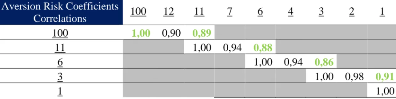
As mentioned before, in order to find the range of risk aversion coefficients that represent the proportion of volatility that is penalized, it was conducted a test of correlation between the outputted ranks. According to University of Strathclyde, if the final rank had a correlation inferior to 0.9, which implies that the correlation is inferior to “perfect” 16_{; it was assumed} that the next number, used as risk aversion coefficient, was a start of a new risk profile.

As demonstrated in Table 5-1, starting with a risk aversion factor of 100, extremely high, representing an investor that, in an exaggerated way, prefers a stable return distribution in his portfolio, rather than aiming at high expected returns, and finishing in an investor with a coefficient of risk aversion equal to 1, it was studied the evolution of the correlation between the ranks that maximize the quadratic utility equation (14).17

Table 5-1 – Aversion Factor Correlation Test between ranks

Aversion Risk Coefficients

Correlations 100 12 11 7 6 4 3 2 1 100 1,00 0,90 0,89 11 1,00 0,94 0,88 6 1,00 0,94 0,86 3 1,00 0,98 0,91 1 1,00

The several “A” factors that were found and that will be used to represent each risk profile are: • Extreme Conservative – ]11 ; ∞[ 100 • Conservative – ]6 ; 11] 11 16_{http://www.strath.ac.uk/aer/materials/4dataanalysisineducationalresearch/unit4/correlationsdirectionandstren} gth/.

17_{The starting “A” number could be higher than 100 but the output results would be similar – a rank with an}

(31)

22 • Moderate – ]3 ; 6] 6

• Moderate Aggressive – ]1 ; 3] 3 • Aggressive – ]0 ; 1] 1

5.2Utility Rankings

Using these risk aversion coefficients ranks were created, based on the utility equation (14), for each risk profile.

5.2.1 Extreme Conservative

For the first risk profile, that can represent an investor with exaggerated conservative preferences, with a risk factor equal to 100, the top ten hedge funds that maximize utility are the following:

Table 5-2 – Rank obtained with Maximization of U with A=100

Ranking Hedge Funds Annualized

Return

Standard

Deviation Utility

1 CATPRICORN FUND-A 6,29% 3,06% 0,02

2 BEAVER CREEK GLOBAL FUND-C 4,01% 2,78% 0,00

3 GABELLI ASSOCIATES LIMITED-A 4,34% 3,11% -0,01

4 NEXTAR FUND-B-GLOBAL FUND 10,29% 5,15% -0,03

5 KBD RELATIVE VALUE VOL-A CON 3,52% 3,70% -0,03

6 ALPHAGEN HOKUTO FND LTD-AUSD 4,86% 4,16% -0,04

7 LIM ASIA MULTI-STRATEGY FD-A 6,63% 5,24% -0,07

8 DELTEC SPECIAL SITUATIONS PR 15,65% 6,79% -0,07

9 TRADELINK GLOBAL EQUITY LP 10,18% 7,14% -0,15

10 NEMROD DIVERSIFIED HLD LTD-A 4,65% 6,32% -0,15

30 THE ADELPHI EUROPE FUND-USD 8,67% 10,07% -0,42

60 LANSDOWNE GLOBAL FINAN-N USD 10,31% 13,59% -0,82

(32)

23 Since the aversion factor is extremely high, just a small amount of volatility is sufficient to penalize return and consequently the value of utility. This rank will award instruments with small amount of volatility rather than great returns, and the composition of this one highly demonstrates this property. In the firsts places are hedge funds with annualized standard deviation around 6%. Conversely, the last ranked ones, despite theirs high rate of returns, have high amounts of volatility that penalize the value of the utility equation.

5.2.2 Conservative

For the second profile and conducting the exact same method, although changing the coefficient of risk aversion to 11, the top ten hedge funds that maximize equation (14) are the following:

Return

Standard

1 DELTEC SPECIAL SITUATIONS PR 15,65% 6,79% 0,13 2 TETON CAPITAL PARTNERS LP 17,30% 12,37% 0,09 3 NEXTAR FUND-B-GLOBAL FUND 10,29% 5,15% 0,09

4 LTE PARTNERS LLC 12,33% 8,21% 0,09

5 SPHERA FUND LP 10,82% 7,65% 0,08

6 GRANITE POINT CAPITAL LP-A 13,11% 10,13% 0,07 7 TRADELINK GLOBAL EQUITY LP 10,18% 7,14% 0,07 8 OCCO EASTERN EUROPEAN FUND-A 10,21% 7,49% 0,07 9 LANSDOWNE DEVELOPED MKT-NRUS 14,27% 11,59% 0,07 10 CAYMUS ENERGY FUND LP 10,21% 7,98% 0,07

30 GALENA FUND LTD-A USD 8,35% 10,23% 0,03

60 MILLBURN MULTI-MKTS TRADING 6,29% 12,24% - 0,02

90 PEAK PARTNERS LP 5,72% 17,02% - 0,10

Comparing this second rank with the previous one, as the aversion factor is considerably smaller and the amount of standard deviation that is penalized is considerably less. So, it is

(33)

24 normal to have hedge funds capable of delivering positive absolute values to the utility equation. Despite the aversion factor being considerably lower, the return distribution of the top ten hedge funds remains conservative. The standard deviation increased when compared to the previous presented rank, but remains low, around 7%.

5.2.3 Moderate

For the third profile, the coefficient of risk aversion that was used was 6, already determined in the beginning of this chapter. The top ten hedge funds that maximize Utility are:

Return

Standard

1 DELTEC SPECIAL SITUATIONS PR 15,65% 6,79% 0,14 2 TETON CAPITAL PARTNERS LP 17,30% 12,37% 0,13

3 LTE PARTNERS LLC 12,33% 8,21% 0,10

4 LANSDOWNE DEVELOPED MKT-NRUS 14,27% 11,59% 0,10 5 GRANITE POINT CAPITAL LP-A 13,11% 10,13% 0,10 6 NEXTAR FUND-B-GLOBAL FUND 10,29% 5,15% 0,09

7 SPHERA FUND LP 10,82% 7,65% 0,09

8 STRATEGOS FUND LP 18,50% 17,93% 0,09

9 TRADELINK GLOBAL EQUITY LP 10,18% 7,14% 0,09 10 OCCO EASTERN EUROPEAN FUND-A 10,21% 7,49% 0,09

30 LIM ASIA MULTI-STRATEGY FD-A 6,63% 5,24% 0,06

60 KBD RELATIVE VALUE VOL-A CON 3,52% 3,70% 0,03

90 APS APAC LONG SHORT FUND-A 8,03% 17,72% - 0,01

When decreasing the aversion risk coefficient, the formula will gradually became more return seeker rather than volatility penalizing. Now the top ten hedge funds are considered less conservative, as standard deviation becomes higher, and the rank will award more the tradeoff between risk and return. The hedge funds that more efficiently reward the risk taken, will be the top ones. Utility values became higher, due to the fact that now the amount of

(34)

25 volatility that is penalized is less than the previous two ranks presented. Now it is more correct to start comparing the return and standard deviation variables. The annualized return of the top ten hedge funds is around 13% and the standard deviation is around 10%. In the bottom of the rank, are instruments that cannot succeed in the remuneration of risk. So as demonstrated the 90th_{position is a fund that carries 17.72% of standard deviation and just} delivers 8.56% of return.

5.2.4 Moderate Aggressive

For the fourth profile, the coefficient of risk aversion utilized was 3 and the top ten hedge funds that maximize equation (14) are the following:

Return

Standard

1 TETON CAPITAL PARTNERS LP 17,30% 12,37% 0,15 2 DELTEC SPECIAL SITUATIONS PR 15,65% 6,79% 0,15

4 LANSDOWNE DEVELOPED MKT-NRUS 14,27% 11,59% 0,12 5 GRANITE POINT CAPITAL LP-A 13,11% 10,13% 0,12 6 VR GLOBAL OFFSHORE FUND LTD 15,57% 16,66% 0,11

7 ARROW PARTNERS LP 15,36% 16,39% 0,11

8 LTE PARTNERS LLC 12,33% 8,21% 0,11

9 THE MERCHANT COMMODITY FUND 18,52% 21,99% 0,11 10 GREEN FUND LLC - GREEN CLASS 14,32% 14,87% 0,11

30 FORT GLOBAL CONTRARIAN PRG 10,05% 10,37% 0,08

60 PERMAL GLOBAL OPPORTUNITE-AQ 7,25% 11,65% 0,05

90 MILLBURN DIVERSIFIED PROGRAM 5,07% 12,16% 0,03

When compared with the previous ones, this rank will start to be more focused on return rather minimizing volatility. The amount of penalization is lower than the previous ones, and so the formula will start, gradually, to award high returns, or considerable returns with lower

(35)

26 standard deviations. In this profile the investor aims the best tradeoff between return and risk, since he is more tolerant to volatility. The top ten hedge funds have an annualized return around 15%, higher than the previous presented but also with higher standard deviation.

5.2.5 Aggressive

The last profile that will be considered in this project has an aversion coefficient of 1, and the top ten Hedge Funds that maximize equation (14) are:

Return

Standard

2 TETON CAPITAL PARTNERS LP 17,30% 12,37% 0,17 3 THE MERCHANT COMMODITY FUND 18,52% 21,99% 0,16 4 DELTEC SPECIAL SITUATIONS PR 15,65% 6,79% 0,15

5 LYNAS ASIA FUND 17,59% 21,66% 0,15

6 GLI FUND LLC-B 17,70% 25,03% 0,15

7 ATTAIN MANAGED FUTURES TREND 16,35% 19,60% 0,14 8 VR GLOBAL OFFSHORE FUND LTD 15,57% 16,66% 0,14

9 ARROW PARTNERS LP 15,36% 16,39% 0,14

10 FORMOSA ASIA OPP-UG GR CMS-A 15,62% 18,87% 0,14

30 NEXTAR FUND-B-GLOBAL FUND 10,29% 5,15% 0,10

60 WORLD MONETARY & AGRICULTURE 11,14% 29,41% 0,07

90 CONTINENTAL PARTNERS LP 6,38% 19,45% 0,04

In this last ranking, investors ignore much part of the variable volatility, seeking high return hedge funds. The instruments that compose the sample that will be chosen for investment are characterized as delivers of return. In this last rank the top ten hedge funds have an annualized return around 17% and also higher standards deviation when compared with the previous ones.

(36)

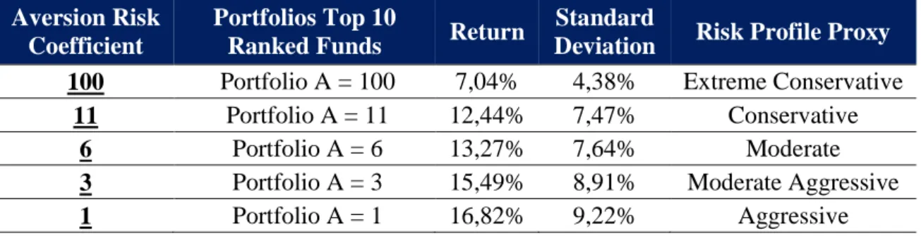
27 The Table 5-8 summarizes the choices that were considered if the top ten hedge funds of each rank were chosen to compose an equal-weighted portfolio. As the investor becomes more risk lover, which translates in more desire to achieve higher returns rather than lower volatility, different instruments become more suited for his preferences.

Table 5-8 – Summary of The Portfolios’ Return and Standard deviation composed by the 10 Top

Ranked Hedge Funds Aversion Risk

Coefficient

Portfolios Top 10

Ranked Funds Return

Standard

Deviation Risk Profile Proxy

100 Portfolio A = 100 7,04% 4,38% Extreme Conservative

11 Portfolio A = 11 12,44% 7,47% Conservative

6 Portfolio A = 6 13,27% 7,64% Moderate

3 Portfolio A = 3 15,49% 8,91% Moderate Aggressive

1 Portfolio A = 1 16,82% 9,22% Aggressive

Figure 5-1 – Accumulated Return over the 10y Period based on the several utility functions.

As Figure 5-1 shows, despite the accumulated return over the 10 year period being lower in the more conservative portfolios, in terms of volatility, these portfolios also carry less risk. In the period of the financial crisis (late 2007 and 2008), most of the high targeted return instruments had high losses, due to more aggressive strategies. Conversely, volatility minimizing funds had lower losses in the same period, that became more suited to conservative investors. 0% 40% 80% 120% 160% 200% 0 1 -1 2 -2 0 0 4 0 1 -0 6 -2 0 0 5 0 1 -1 2 -2 0 0 5 0 1 -0 6 -2 0 0 6 0 1 -1 2 -2 0 0 6 0 1 -0 6 -2 0 0 7 0 1 -1 2 -2 0 0 7 0 1 -0 6 -2 0 0 8 0 1 -1 2 -2 0 0 8 0 1 -0 6 -2 0 0 9 0 1 -1 2 -2 0 0 9 0 1 -0 6 -2 0 1 0 0 1 -1 2 -2 0 1 0 0 1 -0 6 -2 0 1 1 0 1 -1 2 -2 0 1 1 0 1 -0 6 -2 0 1 2 0 1 -1 2 -2 0 1 2 0 1 -0 6 -2 0 1 3 0 1 -1 2 -2 0 1 3 0 1 -0 6 -2 0 1 4 0 1 -1 2 -2 0 1 4

10 years return evolution of the porfolios

Portfolio A = 100 Portfolio A = 11

Portfolio A = 6 Portfolio A = 3 Portfolio A = 1

(37)

28

5.3Performance Measures Ranking

Assuming that every preference of the investor and consequently his utility function were ignored, the process of selection of an instrument that would be considered for investment is through the maximization of traditional performance measures that are already know, and studied. In the next pages it will be presented the ranks that maximize the overall performance measures presented in the previous chapter.

5.3.1 Sharp Ratio

If the Sharp Ratio was the measure that was used in order to select an instrument for investment then the top ten Hedge Funds that would be selected were:

Table 5-9 – Rank based on the maximization of Sharpe Ratio

Return

Standard Deviation

Sharpe Ratio

1 DELTEC SPECIAL SITUATIONS PR 15,65% 6,79% 1,98 2 _{NEXTAR FUND-B-GLOBAL FUND} 10,29% 5,15% 1,58

4 _{LTE PARTNERS LLC} 12,33% 8,21% 1,24

5 TETON CAPITAL PARTNERS LP 17,30% 12,37% 1,22

6 _{SPHERA FUND LP} 10,82% 7,65% 1,13

7 TRADELINK GLOBAL EQUITY LP 10,18% 7,14% 1,12 8 GRANITE POINT CAPITAL LP-A 13,11% 10,13% 1,08 9 OCCO EASTERN EUROPEAN FUND-A 10,21% 7,49% 1,07 10 LANSDOWNE DEVELOPED MKT-NRUS 14,27% 11,59% 1,04

30 GLOBAL DIVERSIFIED SP-CL D 11,70% 13,18% 0,72

60 CARAVEL FUND-ONSHORE 11,07% 17,92% 0,50

90 NEW MILLENNIUM FUNDAMENTAL 6,62% 16,57% 0,27

The top ranked funds are the one that on the basis of risk adjusted return, have higher performance and offer more excess return for an extra unit of volatility by holding the risky

(38)

29 asset. Usually a Sharpe Ratio higher than 1 is considered good, 2 very good and 3 excellent.18 Considering this, the top ten hedge funds are in between good and very good in terms of risk adjusted return. In the bottom of the rank are funds that have a poor tradeoff between risk and return that translate in a Sharpe Ratio inferior to 1.

5.3.2 Sortino Ratio

If the Sortino Ratio was the measure that was used in order to select an instrument for investment then the top ten Hedge Funds that would be selected were:

Table 5-10 – Rank based on the maximization of Sortino Ratio

Return Semi Standard Deviation Sortino Raio

1 DELTEC SPECIAL SITUATIONS PR 15,65% 2,27% 5,94 2 _{NEXTAR FUND-B-GLOBAL FUND} 10,29% 1,95% 4,16

3 LTE PARTNERS LLC 12,33% 3,27% 3,10

4 _{TETON CAPITAL PARTNERS LP} 17,30% 6,46% 2,34 5 PIVOT GLOBAL VALUE FUND-CL A 10,78% 3,68% 2,33 6 _{GRANITE POINT CAPITAL LP-A} 13,11% 4,69% 2,33

7 SPHERA FUND LP 10,82% 3,77% 2,29

9 CAYMUS ENERGY FUND LP 10,21% 3,62% 2,22

10 LANSDOWNE DEVELOPED MKT-NRUS 14,27% 5,78% 2,09

30 LIM ASIA MULTI-STRATEGY FD-A 6,63% 3,22% 1,38

60 SPINNAKER GLOBAL OPPORTUN-K 7,28% 6,40% 0,80

90 1837 PARTNERS LP 6,08% 8,37% 0,47

When using the Sortino ratio, it is possible to remove the implied volatility of the upside movements. So in the top range of this ranking are Hedge Funds that in terms of risk-adjusted return are the best. Risk, in this ratio, has a different interpretation that in the Sharpe Ratio

(39)

30 because the variable that it is used to measure risk is not the standard deviation but the semi standard deviation of the negative returns.

5.3.3 Treynor Ratio

If the Treynor Ratio was the measure that was used in order to select an instrument for investment then the top ten Hedge Funds that would be selected were:

Table 5-11 – Rank based on the maximization of Treynor Ratio

Return Beta

Treynor Ratio

1 DELTEC SPECIAL SITUATIONS PR 15,65% 0,00 32,65

2 GBM GLOBAL LP-B 11,94% 0,07 1,45

3 GABELLI ASSOCIATES LIMITED-A 4,34% 0,02 1,30

4 CARAVEL FUND-ONSHORE 11,07% 0,13 0,66

5 PROSPERITY QUEST SUB FUND-A 13,15% 0,21 0,51

6 _{SPHERA FUND LP} 10,82% 0,25 0,34

7 VERDE GLOBAL MACRO MASTER-GM 8,88% 0,26 0,26 8 _{OCCO EASTERN EUROPEAN FUND-A} 10,21% 0,51 0,16

9 CAYMUS ENERGY FUND LP 10,21% 0,56 0,14

10 _{SPINNAKER GLOBAL EMMKT FND-A} 7,02% 0,35 0,14

30 THE MERCHANT COMMODITY FUND 18,52% 5,73 0,03

60 ROBERTSON OPPORTUNITY FND LP 5,86% -4,16 -0,01

90 _{THE ADELPHI EUROPE FUND-USD} 8,67% -0,98 -0,07

The Treynor ratio, being also a risk-adjusted return performance measure, will compare, in the same way as Sharpe and Sortino, the return of the portfolio, adjusting it with a variable of risk. Contrary to Sharpe and Sortino, the measure of risk that Treynor uses is the systematic one that in finance is known as beta. High beta indicates higher risk and the top hedge funds are the one which in terms of the risk return tradeoff are better to invest.

(40)

31

5.3.4 Information Ratio

If the Information Ratio was the measure that was used in order to select an instrument for investment then the top ten hedge funds that would be selected were:

Table 5-12 – Rank based on the maximization of Information Ratio

Return

Tracking Error

Information Ratio

1 DELTEC SPECIAL SITUATIONS PR 15,65% 6,81% 1,98 2 NEXTAR FUND-B-GLOBAL FUND 10,29% 5,09% 1,59

4 LTE PARTNERS LLC 12,33% 8,30% 1,22

5 TETON CAPITAL PARTNERS LP 17,30% 12,38% 1,22

6 SPHERA FUND LP 10,82% 7,66% 1,13

7 TRADELINK GLOBAL EQUITY LP 10,18% 7,21% 1,11 8 GRANITE POINT CAPITAL LP-A 13,11% 10,16% 1,07 9 OCCO EASTERN EUROPEAN FUND-A 10,21% 7,49% 1,07 10 LANSDOWNE DEVELOPED MKT-NRUS 14,27% 11,53% 1,05

30 GLOBAL DIVERSIFIED SP-CL D 11,70% 13,22% 0,72

60 CARAVEL FUND-ONSHORE 11,07% 17,93% 0,50

90 NEW MILLENNIUM FUNDAMENTAL 6,62% 16,65% 0,27

When using information ratio, the objective is to see the consistency of the portfolio manager. Basically the higher the value of the information Ratio, higher will be the times that the portfolio manager adds excess return over the established benchmark, that in this case is the total return of investing in a risk free instrument represented by the 3 months US LIBOR. In this project, and since the risk free rate is equal to the benchmark, the output of using Information Ratio will be similar to the Sharpe Ratio, since tracking error is similar to the standard deviation.

(41)

32

5.3.5 Maximum Drawdown

If the Maximum Drawdown Ratio was the measure that was used in order to select an instrument for investment then the top ten hedge funds that would be selected were:

Table 5-13 – Rank based on the maximization of Maximum Drawdown Ratio

Return Standard Deviation Maximum Drawdown Ratio

1 BEAVER CREEK GLOBAL FUND-C 4,01% 2,78% -4,15% 2 ALPHAGEN HOKUTO FND LTD-AUSD 4,86% 4,16% -4,80% 3 NEXTAR FUND-B-GLOBAL FUND 10,29% 5,15% -5,57%

4 CATPRICORN FUND-A 6,29% 3,06% -6,25%

5 GABELLI ASSOCIATES LIMITED-A 4,34% 3,11% -6,60% 6 CAYMUS ENERGY FUND LP 10,21% 7,98% -9,54% 7 WINTON FUTURES FUND LTD-BUSD 9,91% 10,95% -9,64% 8 ALPHAGEN VLNTIS FND LTD-AUSD 10,51% 8,59% -11,36% 9 KBD RELATIVE VALUE VOL-A CON 3,52% 3,70% -11,48% 10 GRANITE POINT CAPITAL LP-A 13,11% 10,13% -11,83%

30 PERMAL FXD INC SPECIAL OP-AQ 7,22% 8,68% -20,24%

60 TETON CAPITAL PARTNERS LP 17,30% 12,37% -30,20%

90 NEON LIBERTY EMERG MRKT LP 7,76% 14,64% -48,76%

Maximum Drawdown gives a perspective of risk. When evaluating this measure in a fund, it is important to have the notion how much it is possible, or it was loss, by investing in an instrument. Normally, the strategies that are more conservative are the ones in the top of the ranking.

5.3.6 Modigliani and Modigliani

If the M Squared Ratio was the measure that was used in order to select an instrument for investment then the top ten Hedge Funds that would be selected were:

(42)

33

Table 5-14 – Rank based on the maximization of M square Ratio

Return

Modigliani Ratio

1 DELTEC SPECIAL SITUATIONS PR 15,65% 6,79% 3,39% 2 NEXTAR FUND-B-GLOBAL FUND 10,29% 5,15% 3,14%

3 CATPRICORN FUND-A 6,29% 3,06% 3,00%

4 LTE PARTNERS LLC 12,33% 8,21% 2,93%

5 TETON CAPITAL PARTNERS LP 17,30% 12,37% 2,92%

6 SPHERA FUND LP 10,82% 7,65% 2,87%

7 TRADELINK GLOBAL EQUITY LP 10,18% 7,14% 2,86% 8 GRANITE POINT CAPITAL LP-A 13,11% 10,13% 2,84% 9 OCCO EASTERN EUROPEAN FUND-A 10,21% 7,49% 2,83% 10 LANSDOWNE DEVELOPED MKT-NRUS 14,27% 11,59% 2,82%

30 GLOBAL DIVERSIFIED SP-CL D 11,70% 13,18% 2,62%

60 CARAVEL FUND-ONSHORE 11,07% 17,92% 2,48%

90 NEW MILLENNIUM FUNDAMENTAL 6,62% 16,57% 2,34%

Since interpretation of Sharpe Ratio can be unintuitive, Frank Modigliani and his granddaughter developed a more understandable performance ratio. In terms of this ranking the value of the ratio can be interpreted as the return of the portfolio as if the risk of the portfolio was similar than the risk free asset. So the Top ten Hedge Funds are the ones that have created more excess return on a risk-adjusted basis.

5.3.7 MAR Ratio

If the MAR Ratio was the measure that was used in order to select an instrument for investment then the top ten Hedge Funds that would be selected were:

(43)

34

Table 5-15 – Rank based on the maximization of MAR Ratio

Return

Maximum Drawdown

MAR Ratio

1 NEXTAR FUND-B-GLOBAL FUND 10,29% -5,57% 1,85 2 GRANITE POINT CAPITAL LP-A 13,11% -11,83% 1,11 3 DELTEC SPECIAL SITUATIONS PR 15,65% -14,32% 1,19 4 CAYMUS ENERGY FUND LP 10,21% -9,54% 1,07 5 WINTON FUTURES FUND LTD-BUSD 9,91% -9,64% 1,03 6 ALPHAGEN HOKUTO FND LTD-AUSD 4,86% -4,80% 1,01

7 CATPRICORN FUND-A 6,29% -6,25% 1,01

8 BEAVER CREEK GLOBAL FUND-C 4,01% -4,15% 0,97 9 ALPHAGEN VLNTIS FND LTD-AUSD 10,51% -11,36% 0,93 10 PHARO TRADING FUND LTD 11,60% -13,16% 0,89

30 OCCO EASTERN EUROPEAN FUND-A 10,21% -20,86% 0,49

60 ARMAJARO COMMDTIES FND-A USD 5,87% -21,33% 0,28

90 NEON LIBERTY EMERG MRKT LP 7,76% -48,76% 0,16

The MAR Ratio, being a risk-adjusted performance ratio, will also help understand and compare the return versus the risk undertaken. By adjusting the return to the maximum drawdown, the intuition behind this measure is very similar to risk-adjusted measures.

5.3.8 Skewness

If the Skewness coefficient was the measure that was used in order to select an instrument for investment then the top ten Hedge Funds that would be selected were:

Table 5-16 – Rank based on the maximization of Skewness

Return

Skewness Coefficient

1 PIVOT GLOBAL VALUE FUND-CL A 10,78% 11,50% 1,81 2 ARMAJARO COMMDTIES FND-A USD 5,87% 10,77% 1,64 3 DELTEC SPECIAL SITUATIONS PR 15,65% 6,79% 1,51